Correlation based entanglement criteria for bipartite systems

Abstract

We introduce a class of inequalities based on low order correlations of operators to detect entanglement in bipartite systems. The operators may either be Hermitian or non-Hermitian and are applicable to any physical system or class of states. Testing the criteria on example systems reveals that they outperform other common correlation based criteria, such as those by Duan-Giedke-Cirac-Zoller and Hillery-Zubairy. One unusual feature of the criteria is that the correlations include the density matrix itself, which is related to the purity of the system. We discuss how such a term could be measured in relation to the criteria.

The generation of entanglement is an essential task in quantum information science, and is fundamental to any classically intractable task such as quantum teleportation or quantum computation. Detecting entanglement is therefore an important task that must necessarily be carried out in this context, and is required for benchmarking and characterizing the quantum states created. The simplest system for studying entanglement is the bipartite system. The Peres-Horodecki criterion was first proposed as a necessary condition for all bipartite separable states, and sufficient as well in $2\times 2$ or $2\times 3$ dimensional systems Peres (1996); Horodecki et al. (1996); Horodecki (1997). Beyond such low dimensional systems, sufficient inseparability conditions based on second-order moments have been derived Duan et al. (2000); Simon (2000), which have also been shown necessary for the special case of Gaussian states. However, non-Gaussian states are also crucial in some cases. Some of the entanglement criteria derived so far are based on some forms of uncertainty relations Hofmann and Takeuchi (2003); Gühne (2004); Tóth and Gühne (2005); Hillery and Zubairy (2006); Cavalcanti et al. (2011); He et al. (2011a, b), and especially, in certain cases, in conjunction with partial transposition Shchukin and Vogel (2005) and via SU(1,1) and SU(2) algebra as well Agarwal and Biswas (2005); Nha and Kim (2006); Nha (2007) for non-Gaussian states.

What is particularly useful in the context of experimental verification of entanglement are correlation based witnesses, where a small number of observables are measured, and entanglement can be verified. Examples of such correlation based methods include those by Duan-Giedke-Cirac-Zoller (DGCZ) Duan et al. (2000) and Hillery-Zubairy Hillery and Zubairy (2006). These are used when full tomography of the density matrix is impractical or impossible, and thus only incomplete information of the system is available. Such correlation based methods are typically only a sufficient condition for entanglement, and can fail to detect entanglement across a broad class of entangled states. In this paper, we will introduce another class of correlation based entanglement criteria, which work without assumption of the class of states (Gaussian or non-Gaussian). It is applicable to any physical system and is defined in terms of low-order correlations of Hermitian or non-Hermitian operators. These inequalities do not use any special properties of annihilation operators, allowing for a rather general purpose entanglement witness. Testing the criterion for some typical states we find that it works in a wider range of parameters than similar correlation based methods such as those by DGHZ and Hillery-Zubairy. The use of any type of operator in the criterion is particularly advantageous in comparison to these approaches where certain assumptions need to be satisfied by the observables. The cost of this improvement is that the criteria involves an average over the density matrix squared which can be related to the purity of the system. We discuss how the evaluation of such a term can be evaluated in an experimental setting, together with the performance.

We first introduce and prove the entanglement criterion. Consider a system consisting of two subsystems which is described by a Hilbert space $\mathcal{H}=\mathcal{H}_{a}\otimes\mathcal{H}_{b}$. Let $A_{i}$ be any operator on $\mathcal{H}_{a}$ and $B_{i}$ be any operator on $\mathcal{H}_{b}$ with $i\in\{1,2\}$. Consider the density matrix of a general separable state in diagonal form $\rho=\sum_{k}p_{k}|k\rangle_{a}\langle k|_{a}\otimes|k\rangle_{b}\langle k|_{b}$, where $p_{k}$ is a probability $\sum_{k}p_{k}=1$. The states $|k\rangle_{a,b}$ on subsystems $a$ or $b$ are not necessarily orthogonal $\langle k|k^{\prime}\rangle_{a,b}\neq\delta_{kk^{\prime}}$, but are normalized. We define

$$U=(A_{1})^{\sigma_{A_{1}}}|k\rangle_{a}\langle k|_{a}(A_{1}^{\dagger})^{\bar{\sigma}_{A_{1}}}\otimes(B_{1})^{\sigma_{B_{1}}}|l\rangle_{b}\langle l|_{b}(B_{1}^{\dagger})^{\bar{\sigma}_{B_{1}}},$$

$$V=(A_{2})^{\sigma_{A_{2}}}|l\rangle_{a}\langle l|_{a}(A_{2}^{\dagger})^{\bar{\sigma}_{A_{2}}}\otimes(B_{2})^{\sigma_{B_{2}}}|k\rangle_{b}\langle k|_{b}(B_{2}^{\dagger})^{\bar{\sigma}_{B_{2}}}.$$ (1)

The $\sigma_{A_{i},B_{i}}=\{0,1\}$ are binary parameters which serve to adjust the position of the operators and $\bar{\sigma}_{A_{i},B_{i}}=1-\sigma_{A_{i},B_{i}}$. Now consider the quantity $Z^{\dagger}Z$, where $Z=U-e^{i\phi}V$ and $\phi$ is a free parameter. Since $Z^{\dagger}Z$ is a semi-positive Hermitian operator, which means $\text{Tr}(Z^{\dagger}Z)\geq 0$, and $\sum_{k,l}p_{k}p_{l}\text{Tr}(Z^{\dagger}Z)\geq 0$ will always hold. Then for separable states, we have

$$\langle n_{A_{1}}\rangle\langle n_{B_{1}}\rangle+\langle n_{A_{2}}\rangle\langle n_{B_{2}}\rangle$$

$$-e^{i\phi}\text{Tr}\Big{[}(A_{1}^{\dagger})^{\sigma_{A_{1}}}(A_{2})^{\sigma_{A_{2}}}(B_{2}^{\dagger})^{\bar{\sigma}_{B_{2}}}(B_{1})^{\bar{\sigma}_{B_{1}}}\rho$$

$$\times(A_{2}^{\dagger})^{\bar{\sigma}_{A_{2}}}(A_{1})^{\bar{\sigma}_{A_{1}}}(B_{1}^{\dagger})^{\sigma_{B_{1}}}(B_{2})^{\sigma_{B_{2}}}\rho\Big{]}$$

$$-e^{-i\phi}\text{Tr}\Big{[}(A_{2}^{\dagger})^{\sigma_{A_{2}}}(A_{1})^{\sigma_{A_{1}}}(B_{1}^{\dagger})^{\bar{\sigma}_{B_{1}}}(B_{2})^{\bar{\sigma}_{B_{2}}}\rho$$

$$(A_{1}^{\dagger})^{\bar{\sigma}_{A_{1}}}(A_{2})^{\bar{\sigma}_{A_{2}}}(B_{2}^{\dagger})^{\sigma_{B_{2}}}(B_{1})^{\sigma_{B_{1}}}\rho\Big{]}\geq 0.$$ (2)

where $n_{A_{i}}=A_{i}^{\dagger}A_{i}$ and $n_{B_{i}}=B_{i}^{\dagger}B_{i}$. As $A_{i}$ and $B_{i}$ are arbitrary operators, which can be either Hermitian or non-Hermitian, $n$ may or may not be number operators. Eq. (2) is true for any separable state. Hence, any violation of (2) shows that a state is entangled.

Similarly, we may define

$$U =(A_{1})^{\sigma_{A_{1}}}|k\rangle_{a}\langle k|_{a}(A_{1}^{\dagger})^{\bar{\sigma}_{A_{1}}}\otimes(B_{1})^{\sigma_{B_{1}}}|k\rangle_{b}\langle k|_{b}(B_{1}^{\dagger})^{\bar{\sigma}_{B_{1}}},$$

$$V =(A_{2})^{\sigma_{A_{2}}}|l\rangle_{a}\langle l|_{a}(A_{2}^{\dagger})^{\bar{\sigma}_{A_{2}}}\otimes(B_{2})^{\sigma_{B_{2}}}|l\rangle_{b}\langle l|_{b}(B_{2}^{\dagger})^{\bar{\sigma}_{B_{2}}}.$$ (3)

which is the same as (1) except that the $k$ and $l$ labels are interchanged on subsystem $b$. Using the same steps we obtain the inequality

$$\langle n_{A_{1}}n_{B_{1}}\rangle+\langle n_{A_{2}}n_{B_{2}}\rangle$$

$$-e^{i\phi}\text{Tr}\Big{[}(A_{1}^{\dagger})^{\sigma_{A_{1}}}(A_{2})^{\sigma_{A_{2}}}(B_{1}^{\dagger})^{\sigma_{B_{1}}}(B_{2})^{\sigma_{B_{2}}}\rho$$

$$\times(A_{2}^{\dagger})^{\bar{\sigma}_{A_{2}}}(A_{1})^{\bar{\sigma}_{A_{1}}}(B_{2}^{\dagger})^{\bar{\sigma}_{B_{2}}}(B_{1})^{\bar{\sigma}_{B_{1}}}\rho\Big{]}$$

$$-e^{-i\phi}\text{Tr}\Big{[}(A_{2}^{\dagger})^{\sigma_{A_{2}}}(A_{1})^{\sigma_{A_{1}}}(B_{2}^{\dagger})^{\sigma_{B_{2}}}(B_{1})^{\sigma_{B_{1}}}\rho$$

$$(A_{1}^{\dagger})^{\bar{\sigma}_{A_{1}}}(A_{2})^{\bar{\sigma}_{A_{2}}}(B_{1}^{\dagger})^{\bar{\sigma}_{B_{1}}}(B_{2})^{\bar{\sigma}_{B_{2}}}\rho\Big{]}\geq 0.$$ (4)

Again, any violation of (4) shows that the state is entangled.

The inequalities (2) and (4) are our main result. To illustrate their utility, let us consider a few special cases. Setting $A_{i}=A$, $B_{i}=B$, $\sigma_{A_{i}}=1$, $\sigma_{B_{i}}=0$, and $\phi=0$, Eq. (2) reduces to

$$\langle n_{A}\rangle\langle n_{B}\rangle\geq\langle n_{A}n_{B}\rho\rangle.$$ (5)

where $\langle X\rho Y\rangle\equiv\text{Tr}(X\rho Y\rho)$ for any operators $X,Y$. Another example is $A_{i}=A$, $B_{i}=B$, and $\sigma_{A_{1}}=\sigma_{B_{2}}=1$, $\sigma_{A_{2}}=\sigma_{B_{1}}=0$ in Eq. (4), for which we obtain

$$2\langle n_{A}n_{B}\rangle\geq e^{i\phi}\langle A^{\dagger}B\rho A^{\dagger}B\rangle+e^{-i\phi}\langle AB^{\dagger}\rho AB^{\dagger}\rangle.$$ (6)

We can thus generate a whole family of inequalities which all serve as entanglement witnesses by various choices of $\sigma$ and operators. The phase $\phi$ can be chosen in such a way such that the last two terms in (2) and (4) take its largest negative value, which gives the best chance of violating the inequality. We note that for any pure state, we have $\rho^{2}=\rho$ so that (5) reduces to the ordinary correlation function $\langle n_{A}\rangle\langle n_{B}\rangle-\langle n_{A}n_{B}\rangle$, which has known connections to entanglement for pure states Barnum et al. (2004); Somma et al. (2004). Meanwhile (6) reduces to $2\langle n_{A}n_{B}\rangle\geq e^{i\phi}\langle A^{\dagger}B\rangle^{2}+e^{-i\phi}\langle AB^{\dagger}\rangle^{2}$.

The unusual feature of the criteria that we consider in this paper is that the density matrix is involved in the correlations themselves. The origin of this is that in the terms involving a trace in (2) and (4) there are two density matrices. While this makes evaluation of the correlations slightly less convenient than an ordinary expectation value, this helps to make our entanglement criterion more sensitive than existing correlation based criteria. On first glance it may appear that evaluation of such a term would require knowledge of the full density matrix via tomography, which defeats the purpose of a correlation based entanglement witness. We now show two strategies that can estimate this term without full tomography. We will focus upon the specific case of (5) as this is the criterion which we have found to be simplest and also most sensitive for various states that we have examined.

The first of the methods involves a measurement of the observable $X=n_{A}n_{B}$ combined with some simple post-processing. Our aim will be to obtain an estimator for $\langle X\rho\rangle$, which we will call ${\cal E}(X,\rho)$. The aim of any estimator is that it should give a reasonable approximation to the desired quantity, i.e. ${\cal E}(X,\rho)\approx\langle X\rho\rangle$. Furthermore, in the context of the criterion (5) we would like that ${\cal E}(X,\rho)\leq\langle X\rho\rangle$, in order that estimator can replace the $\langle n_{A}n_{B}\rho\rangle$ term. Let $X$ be an operator which can be expanded in terms of its eigenstates as $X=\sum_{n}X_{n}|X_{n}\rangle\langle X_{n}|$, where $|X_{n}\rangle$ and $X_{n}$ are the $n$th eigenstate and eigenvalue respectively. Now consider making a measurement of the state $\rho$ with respect to $X$. The particular outcome $n$ will be obtained with probability $P_{n}=\text{Tr}(|X_{n}\rangle\langle X_{n}|\rho)$. We then propose that an estimator for $\langle X\rho\rangle$ is

$${\cal E}(X,\rho)=\sum_{n}P_{n}^{2}X_{n}.$$ (7)

To show that the estimator has the desired properties, write the density matrix in its diagonal form $\rho=\sum_{k}p_{k}|\Psi_{k}\rangle\langle\Psi_{k}|$. We may evaluate that

$$\langle X\rho\rangle =\sum_{n}\sum_{k}p_{k}^{2}|\langle\Psi_{k}|X_{n}\rangle|^{2}X_{n},$$ (8)

$${\cal E}(X,\rho) =\sum_{n}\big{(}\sum_{k}p_{k}|\langle\Psi_{k}|X_{n}\rangle|^{2}\big{)}^{2}X_{n}.$$ (9)

Under the condition that $|X_{n}\rangle=|\Psi_{n}\rangle$, these two expressions coincide. Such conditions can be satisfied by either making a choice of measurement $A,B$ such that the eigenstates of $n_{A}n_{B}$ coincides with the state being prepared. Alternatively, for very mixed states $\rho\approx I/d$ where $d$ is the dimension of the system, the choice of basis can be made arbitrarily, and the estimator agrees with the desired expression. Thus we expect such an estimator to give a good approximation for states with low purity. By looking at the difference $\langle X\rho\rangle-{\cal E}(X,\rho)$ and taking $|\langle\Psi_{k}|X_{n}\rangle|^{2}$ to be a probability distribution, it can be shown that ${\cal E}(X,\rho)\leq\langle X\rho\rangle$ as it is a sum of variances. Thus (7) has the desired properties of an estimator and does not require a full tomography of the density matrix.

The second approach is based on the observation that $\langle X\rho\rangle=\text{Tr}(X\rho^{2})$ is a quantity that is closely related to the purity $\text{Tr}(\rho^{2})$. We may then construct another estimator

$${\cal E}(X,\rho)=\langle X\rangle\text{Tr}(\rho^{2}),$$ (10)

which is a mean field approximation in $X$ and $\rho$. Since for a pure state $\langle X\rho\rangle=\langle X\rangle$, we expect that this estimator should work in the opposite limit to that of (7), which is more appropriate for strongly mixed states. Again in the context of our criterion we require that the estimator underestimate the actual $\langle X\rho\rangle$. While this is not generally true of (10), under particular conditions this may be satisfied. To see this, consider a nearly pure state

$$\rho=p|\Psi_{0}\rangle\langle\Psi_{0}|+(1-p)|\Psi_{1}\rangle\langle\Psi_{1}|,$$ (11)

where $|\Psi_{0}\rangle$ can be thought as being the target state, and $|\Psi_{1}\rangle$ is some undesired noise state. For this case we can evaluate that

$$\langle X\rho\rangle-{\cal E}(X,\rho)=(1-p)p(2p-1)(\langle X\rangle_{0}-\langle X\rangle_{1}),$$ (12)

where $\langle X\rangle_{k}=\langle\Psi_{k}|X|\Psi_{k}\rangle$. For $1/2<p\leq 1$, this is a positive quantity if $\langle X\rangle_{0}\geq\langle X\rangle_{1}$ as desired. In this case we can use the estimator (10) conditionally, when some information of the desired and noise states of the system are known.

Writing the estimator in the form of (10) requires an estimate of the purity of the system $\text{Tr}(\rho^{2})$. This has been investigated in many past works, we quote several approaches here which give a relatively simple way of estimating it. The purity may be obtained by summing over variances or expectation values of observables according to

$$\text{Tr}(\rho^{2}) =d-\sum_{l}\delta(M_{l})^{2}=\sum_{l}|\langle M_{l}\rangle|^{2}$$ (13)

where the observables $M_{k}$ satisfy $\text{Tr}(M_{k}M_{l})=\delta_{kl}$ Gühne et al. (2007). This is tractable for low-dimensional systems such as qubits, but for infinite dimensional systems such as photons is unsuitable due to the large number of observables. For such systems, an estimate of the purity may be obtained from the covariance matrix $C$. For photonic Gaussian states the purity is given by $\text{Tr}(\rho^{2})=1/\sqrt{\text{Det}(C)}$ where for a two mode state $C$ is the submatrix with cross-correlations between the modes Tahira et al. (2009); Kogias et al. (2015); Man’ko et al. (2011). In addition, several theoretical and experimental works show methods for directly measuring purity by creating two copies of the system, and interfering them with each other Islam et al. (2015); Bartkiewicz et al. (2013).

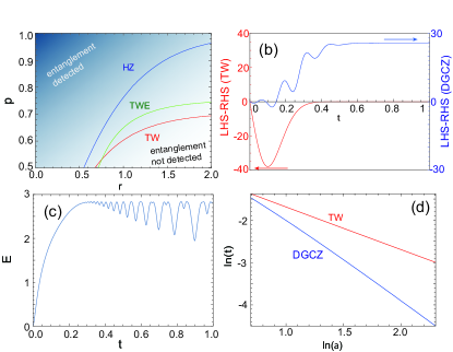
Figure 1: (a) Regions of parameter space for the mixed two mode squeezed state (15) where entanglement is detected for several criteria as marked. HZ corresponds to the Hillery-Zubairy criterion $|\langle ab\rangle|^{2}>\langle n_{a}\rangle\langle n_{b}\rangle$ (entangled); TW (this work) corresponds to (5); TWE (this work with estimator) corresponds to using (5) with (10). (b) Violation of the entanglement criteria for evolution of two coherent states $|\alpha\rangle_{a}|\beta\rangle_{b}$ under a cross-Kerr Hamiltonian $H=n_{a}n_{b}$ for a time $t$. For the two criteria (5) and (19) the LHS-RHS is plotted, such that a violation of the inequality (and therefore entanglement) is negative. Parameters used are $\alpha=\beta=5$. (c) Entropy of entanglement as a function of time $t$ for cross-Kerr Hamiltonian, with $\alpha=\beta=5$. (d) Scaling of the criteria (5) and (19) as a function of $\alpha=\beta$. TW corresponds to the time where LHS-RHS is a minimum for (5); DGCZ corresponds to the time where (19) has LHS=RHS.

We now apply our criterion to several examples and compare the performance with other correlation based entanglement witnesses. In our first example we apply our methods to the Bell states

$$|{\cal B}_{1}\rangle=\frac{1}{\sqrt{2}}(|1\rangle_{a}|0\rangle_{b}+|0\rangle_{a}|1\rangle_{b}),$$

$$|{\cal B}_{2}\rangle=\frac{1}{\sqrt{2}}(|0\rangle_{a}|0\rangle_{b}+|1\rangle_{a}|1\rangle_{b}).$$ (14)

Specifically, we apply the criterion (5) taking $A=\sigma_{a}^{-}$ and $B=\sigma_{b}^{-}$, where $\sigma^{-}$ is a Pauli spin lowering operator. For either Bell state, simple evaluation of (5) shows a violation of the inequality, signalling entanglement. We note that using the Hillery-Zubairy criteria, while $|{\cal B}_{1}\rangle$ shows entanglement, $|{\cal B}_{2}\rangle$ does not, as these are treated using two separate inequalities. In an optics setting, $|{\cal B}_{1}\rangle$ corresponds to beam splitter type of entanglement, while $|{\cal B}_{2}\rangle$ corresponds to parametric down conversion, which have two different criteria for the Hillery-Zubairy approach.

For mixed qubit states, we consider the Werner state $\rho_{i}=p|{\cal B}_{i}\rangle\langle{\cal B}_{i}|+I(1-p)/4$, where $0\leq p\leq 1$, $i=1,2$, and $I$ is the identity operator. Using our criteria (5) we obtain that the state is entangled in the range $0.6<p\leq 1$. For comparison, the Hillery-Zubairy criterion gives entanglement in the range $(\sqrt{5}-1)/2\hskip 5.69054pt(\approx 0.62)<p\leq 1$ (the criterion (6) gives exactly this same range). Thus our criterion (5) provides a slightly wider range of entanglement detection for qubits. We note that other criteria such the Peres-Horodecki (positivity under partial transpose) criterion Horodecki et al. (1996) do give a larger range of entanglement detection $1/3<p\leq 1$. However, this is not a correlation based method and can be expected in general to perform better as it uses the complete information available in the density matrix.

The second example is a mixed state consisting of a two-mode squeezed vacuum state $|r\rangle$ and a thermal state on each mode $\rho_{\text{th}}^{a,b}$, with density matrix

$$\rho =p|r\rangle\langle r|+(1-p)\rho_{\text{th}}^{a}\otimes\rho_{\text{th}}^{b}$$ (15)

$$|r\rangle =\sqrt{1-\tanh^{2}(r)}\sum_{n}\tanh^{n}(r)|n\rangle_{a}|n\rangle_{b}$$

$$\rho_{\text{th}}^{a,b} =(1-\tanh^{2}(r))\sum_{n}\tanh^{2n}(r)|n\rangle_{a,b}\langle n|_{a,b},$$ (16)

where $r$ is the squeezing parameter, and we have assumed that the thermal state has the same thermal characteristics as the squeezing parameter due to some decoherence in the system. The result of using our criterion (5) is shown in Fig. 1(a). From the calculation of the negativity Vidal and Werner (2002); Życzkowski et al. (1998), we find that the state (15) is always entangled for any $p>0$. Our criterion shows that the state is entangled in a large portion of the parameter space, and indicates that it is a sensitive detector of entanglement. In comparison, the Hillery-Zubairy criterion shows a smaller range of parameters that reveal entanglement. The dashed line in Fig. 1(a) represents the bound that would be obtained by the application of the second estimator (10). While the range of entanglement is reduced, it still shows a larger range than the Hillery-Zubairy approach. We note the estimator must be used conditionally where the $\langle n_{A}n_{B}\rangle$ is larger for the squeezed state than the thermal state and $p>1/2$, hence works only in a restricted region.

The third example we show is entanglement due to a cross-Kerr nonlinearity Schmidt and Imamoglu (1996), which exhibits non-Gaussian characteristics. Evolving the Hamiltonian $H=n_{a}n_{b}$ for a time $t$ gives Heisenberg equations as

$$p_{a}(t)\approx p_{a}(0)-tx_{a}(0)n_{b}(0),$$

$$x_{a}(t)\approx x_{a}(0)+tp_{a}(0)n_{b}(0),$$ (17)

and similarly with $a\leftrightarrow b$. Taking two initially coherent states $|\alpha\rangle_{a}|\beta\rangle_{b}$ where $\alpha,\beta$ are real and positive, we expect that initially correlations between $p_{a}$ and $n_{b}$ should develop, as $x_{a}(0)\approx\alpha$ and $x_{b}(0)\approx\beta$. At later times when $p_{a}$ is not necessarily small, we also expect that correlations between $x_{a}$ and $n_{b}$ should also be present. More generally, we expect that correlations between operators

$$A=\frac{1}{2}(e^{-i\theta}a^{\dagger}+e^{i\theta}a),\quad B=b$$ (18)

are present, where $a,b$ are annihilation operators for mode $a$ and $b$, and $\theta$ is a free parameter that may be optimized. $B$ could equally be taken as $n_{b}$, however, we find that the above choice works equally well (Fig. 1(b)). Our criterion detects entanglement for all $t$ except $t=2\pi n$ where $n$ is an integer, where the state becomes disentangled again. This can be compared to a calculation of the entropy in Fig.1(c) which reveals that entanglement is present for the same times. The entropy has a fractal form that is reminiscent of the ”Devil’s crevasse” entanglement as seen in entangled spinor Bose-Einstein condensates Byrnes (2013). We note that the violation is only significant for $t\sim 1/|\alpha|$ (and similar periodic times) for $\alpha=\beta$ hence in practice may only be effective in this region.

Applying the Hillery-Zubairy criterion to the cross-Kerr case with operators (18) reveals no entanglement for all $t$. This is due to the fact that one of the operators is Hermitian, for which the separability inequality can never be violated. The DGCZ criterion can however detect entanglement Wang et al. (2015). Choosing similar operators and following the same procedure as in Ref. Duan et al. (2000) gives the criterion for separable states

$$\delta(p_{a}+\tau t\alpha n_{b})^{2}+\delta(p_{b}+\tau^{\prime}t\beta n_{a})^{2}\geq|\tau^{\prime}t\beta\langle x_{a}\rangle|+|\tau t\alpha\langle x_{b}\rangle|$$ (19)

where $\tau$ and $\tau^{\prime}$ are parameters that can be optimized. From Fig. 1(b) we see that beyond short times $t\ll 1/\alpha$, entanglement cannot be detected using the DGCZ criterion. We attribute this to the strongly non-Gaussian nature of the states that are generated using the cross Kerr nonlinearity. In deriving the DGCZ inequality, a postion-momentum type Heisenberg uncertainly relation is used, which is not necessarily the relevant relation for strongly non-Gaussian states. In Fig. 1(d) we examine the dependence of characteristic times with the coherent state amplitude for our criterion and DGCZ. For the DGCZ criterion we plot the time where entanglement is no longer is detected, while for our criterion we plot the time where the maximum violation is achieved. We find that the scaling of our relation follows a power law as $t\propto 1/|\alpha|$, while the DGCZ criterion falls off at a faster rate than $t\propto 1/|\alpha|^{2}$. This shows that our criterion works in a considerably larger range of times, particularly as the amplitude of the coherent state is increased.

In summary, we have derived a correlation based entanglement witness for bipartite systems. The criterion works with an arbitrary pair of observables on each of the subsystems. We have compared the performance with other correlation based criteria, and find that in many cases it detects entanglement in a larger range of parameters than similar methods such as those of Hillery-Zubairy and Duan-Giedke-Cirac-Zoller. The cost of this improvement is the necessity to evaluate a correlation involving the density matrix itself, which is related to the purity of the system. We provide several methods of estimating this term, and find that it is possible under several circumstances to do so in a way that reduces the effectiveness of the criterion in a minimal way. We have investigated primarily the case (5) which is a special case of the family of inequalities (2) and (4). Due to the great flexibility of the general expression, there is much scope for further investigation of other criteria using different combinations of operators. This may lead to more sensitive entanglement criteria, particularly for strongly non-Gaussian states which are less easy to detect using correlations based methods.