Self-Consistent Field Theory studies of the thermodynamics and quantum spin dynamics of magnetic Skyrmions

Abstract

A self-consistent field theory is introduced and used to investigate the thermodynamics and spin dynamics of an $S=1$ quantum spin system with a magnetic Skyrmion. The temperature dependence of the Skyrmion profile as well as the phase diagram are calculated. It is shown that the Skyrmion carries a phase transition to the ferromagnetic phase of first order with increasing temperature, while the magnetization of the surrounding ferromagnet undergoes a phase transition of second order when changing to the paramagnetic phase. Furthermore, the electric field driven annihilation process of the Skyrmion is described quantum mechanical by solving the time dependent Schrödinger equation. The results are compared with the trajectories of the semi-classical description of the spin expectation values using a differential equation similar to the classical Landau-Lifshitz-Gilbert equation.

I Introduction

Magnetic Skyrmions have undergone an intensive attention during the last years caused by the ideas to use them for data storage and as part of logic devices Zhang et al. (2015a); Zhou and Ezawa (2014); Fert et al. (2013); Zhang et al. (2015b, c). The advantage of magnetic Skyrmions is the stability due to their topology. Secondly, magnetic Skyrmions are smaller than other domain wall formations and therefore a higher storage density and a faster information flow are possible Fert et al. (2013). Furthermore, magnetic Skyrmions can be found in magnetic film systems at the atomic length Romming et al. (2013); Barker and Tretiakov (2016) scale as well as in magnetic films with micrometer dimensions Jiang et al. (2015); Woo et al. (2016); Mühlbauer et al. (2009). This makes it possible to design devices on several length scales or to combine these scales.

So far all computer simulations describing the dynamics of magnetic Skyrmions using a classical description. Furthermore there are only a hand full theoretical studies investigating the thermodynamics of Skyrmions. However, Usov et al. N. A. Usov and S. A. Gudoshnikov (2005) and Nieves et al. Nieves et al. (2014) have pointed out that a classical description is not always convenient. Within this publication a quantum mechanical self-consistent field (SCF) theory using a Hartree-Fock approximation is used to describe the thermodynamics and after further modification to describe the spin dynamics of a single Skyrmion.

SCF theories in general offer the chance to investigate complex many-body systems by reducing them to local one-body problems. This fact together with the dispelling of the fluctuations make these theories successful. So far, several theories like the Ginzburg-Landau theory Stanley (1971); Coey (2009), the Stoner model of itinerant magnets W. Nolting and A. Ramakanth (2010), the random phase approximation (RPA) in the description of many-body Green’s functions W. Nolting and A. Ramakanth (2010), the Hartree-Fock theory Levine (1991); Piela (2007), and some other theories have been proposed using the same methodology.

The within this study used quantum mechanical SCF theory helps to increase the system size which can be addressed. Actually it is possible via exact diagonalization to describe the dynamics and thermodynamics of 60 quantum spins with spin quantum number $S=1/2$ on a square lattice. With the SCF theory the description becomes local and entanglement among the spins plays no role. Therefore, the Hilbert space and the corresponding matrices of the system are drastically reduced and larger system sizes can be addressed: within this publication e.g. $200\times 200=40000$ quantum spins $S=1$ on a quadratic lattice. However, the used theory makes sense only if entanglement is negligible. In systems with strong entanglement the SCF theory will lead to false results.

The publication is organized as follow: In Sec. II the quantum mechanical SCF Hamilton operator $\hat{\mathrm{H}}$ is introduced. Sec. III describes the temperature dependence of the local magnetization inside and outside the Skyrmion. The eigenvalue and eigenfunction of the ground state of the Hamiltonian $\hat{\mathrm{H}}$ are discussed in Sec. IV and Sec. V describes the switching dynamics of the Skyrmion driven by an electric field oriented perpendicular to the film plane. The publication ends with a summary (Sec. VI).

II Model

The quantum mechanical SCF theory using a Hartree-Fock approximation is used to describe a single magnetic Skyrmion. So far, nearly all studies investigating magnetic Skyrmions using the classical Heisenberg model or the micromagnetic approximation of the Heisenberg model. However, the classical approach is not always flexible enough to study the magnetic properties N. A. Usov and S. A. Gudoshnikov (2005); Nieves et al. (2014). The description within this study is quantum mechanical and investigates a square lattice with $200\times 200$ quantum spins with spin quantum number $S=1$. The physical properties are described by the following Hamilton operator:

$$\hat{\mathrm{H}}= - J\sum\limits_{n,m}\hat{\mathbf{S}}_{n}\cdot\langle\hat{\mathbf{S}}_{m}\rangle-\sum\limits_{n,m}{\boldsymbol{\cal D}}_{nm}\cdot(\hat{\mathbf{S}}_{n}\times\langle\hat{\mathbf{S}}_{m}\rangle)$$ (1)

$$- g\mu_{B}\sum\limits_{n}\mathbf{B}\cdot\hat{\mathbf{S}}_{n}\;.$$

$\hat{\mathrm{H}}$ describes the interaction of the spin operator $\hat{\mathbf{S}}_{n}$ with the surrounding spins by their expectation values $\langle\hat{\mathbf{S}}_{m}\rangle$. Therefore, the description is reduced to a description of local spins.

The first and second terms of the Hamilton operator $\hat{\mathrm{H}}$ describe the nearest neighbor exchange and Dzyaloshinsky-Moriya interaction. Depending on the sign the exchange interaction is either ferromagnetic $J>0$ or antiferromagnetic $J<0$. In the following a ferromagnetic interaction is assumed. Together with the exchange interaction the Dzyaloshinsky-Moriya interaction (DMI) lead to a spin-spiral. The ${\boldsymbol{\cal D}}_{nm}$ are the DMI vectors responsible for the direction and sense of rotation of the spiral Dzyaloshinsky (1985); Crépiex and Lacroix (1998). Within this publication the ${\boldsymbol{\cal D}}_{nm}$ are assumed to be in-plane (magnetic film) vectors oriented perpendicular to the connection between two nearest neighbor lattice sites: ${\boldsymbol{\cal D}}_{nm}\perp\mathbf{r}_{nm}$. The third term in $\hat{\mathrm{H}}$ describes the coupling of the spins to an external magnetic field (Zeeman term). Within this term $g$ is the Landé factor, $\mu_{B}$ the Bohr magneton, and $\mathbf{B}$ the magnetic field. In the following an external magnetic field perpendicular to the film plane ($z$-direction) is assumed to stabilize the Skyrmion. The resulting Skyrmion can be seen in Fig. 1. The values for the the ferromagnetic exchange interaction, the DMI and external field used in this study are $J=7$ meV, ${\cal D}_{nm}=2.2$ meV, and $B=4.5$ T.

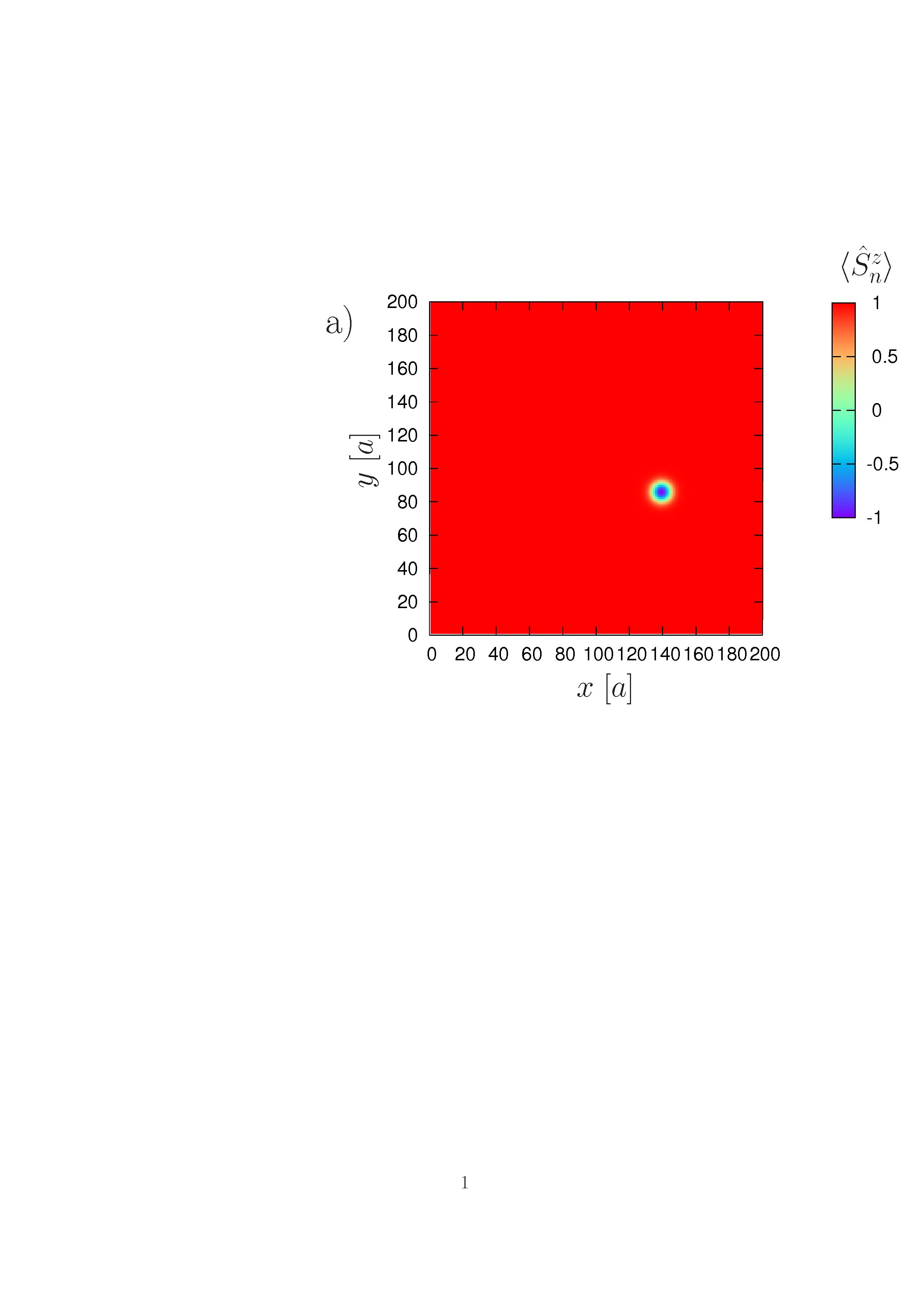
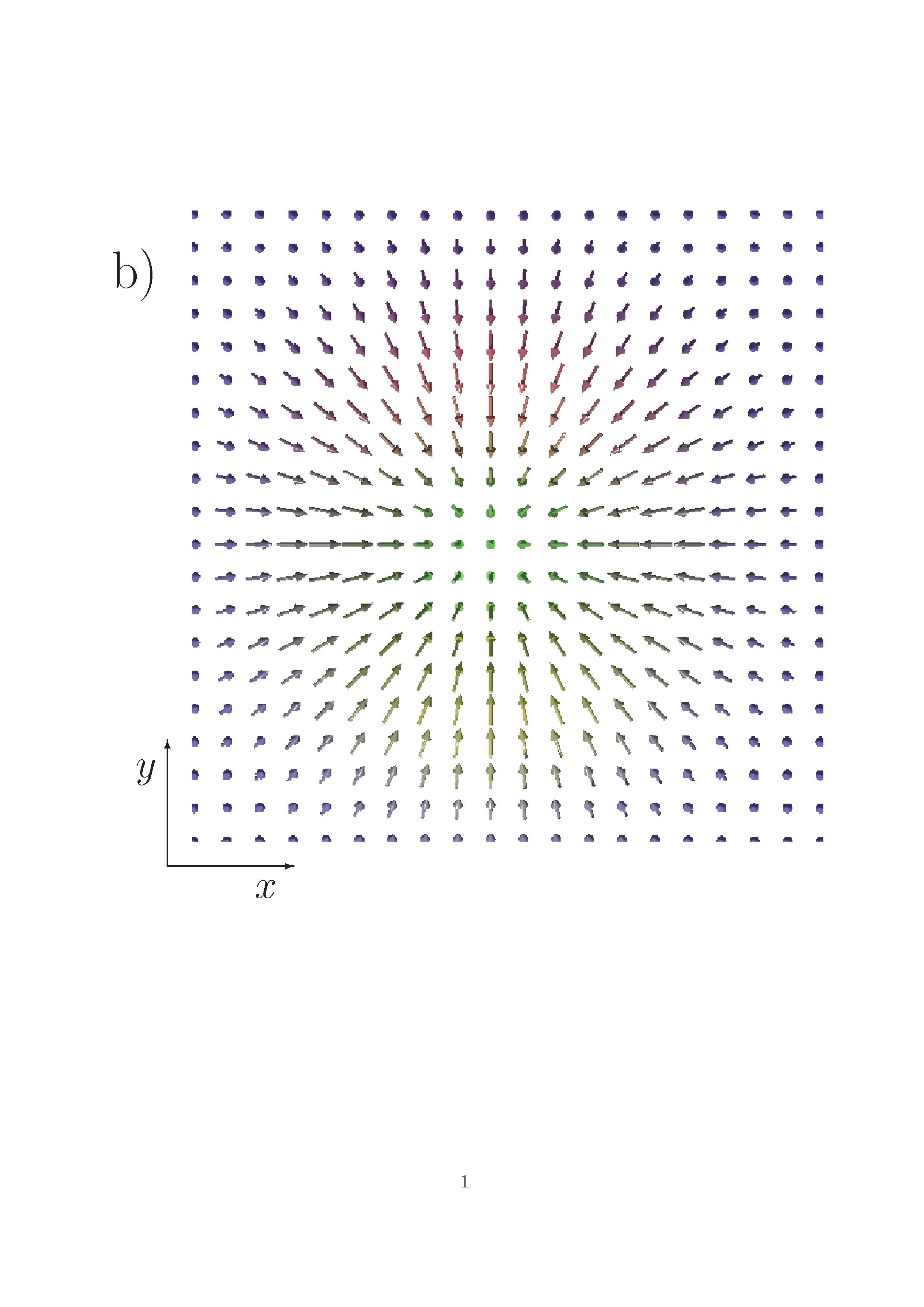
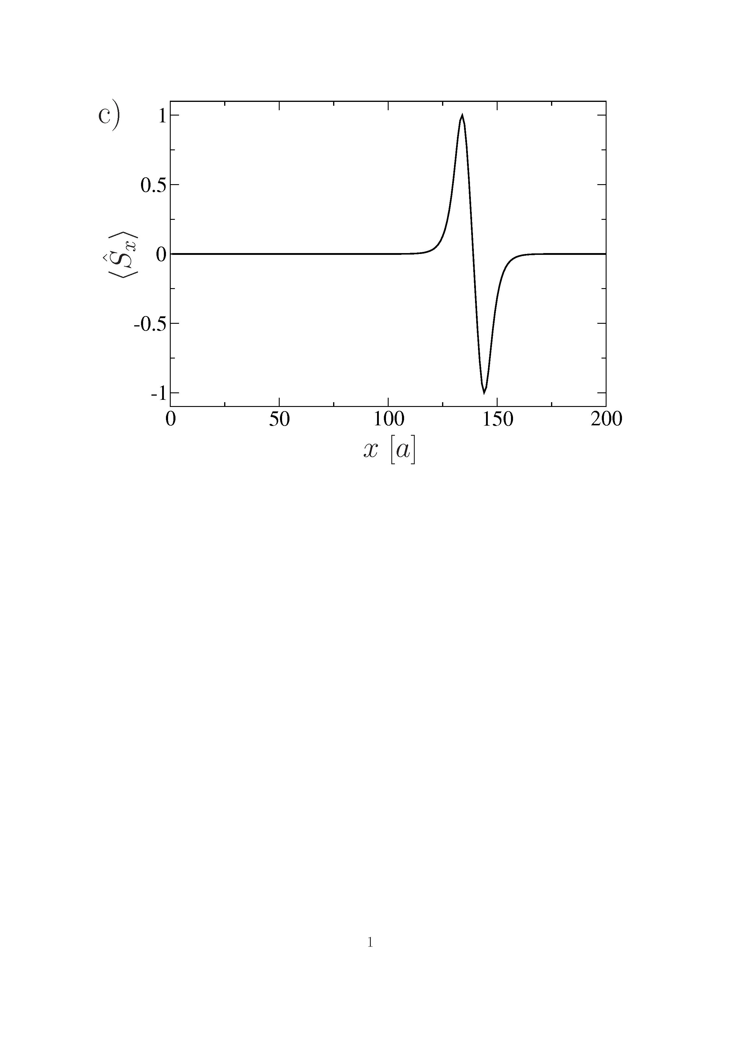
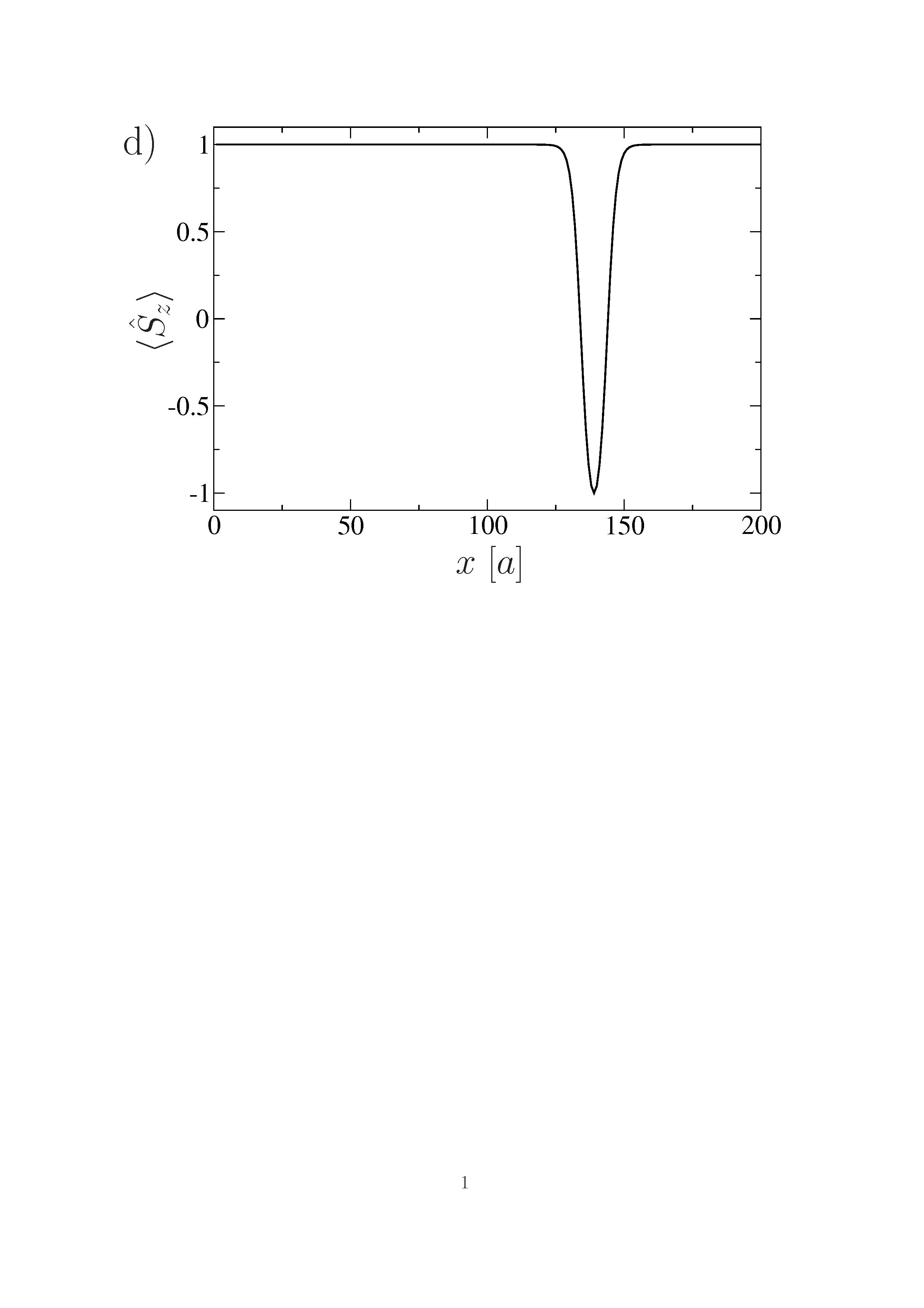
Figure 1: (color online) Single magnetic Skyrmion: a) $z$-component, b) in plane Hedgehog structure, c) and d) corresponding profiles provided by a cut through the center of the Skyrmion. The Skyrmion structure and profiles are calculated with Eq. (6) at $B=4.5$ T.

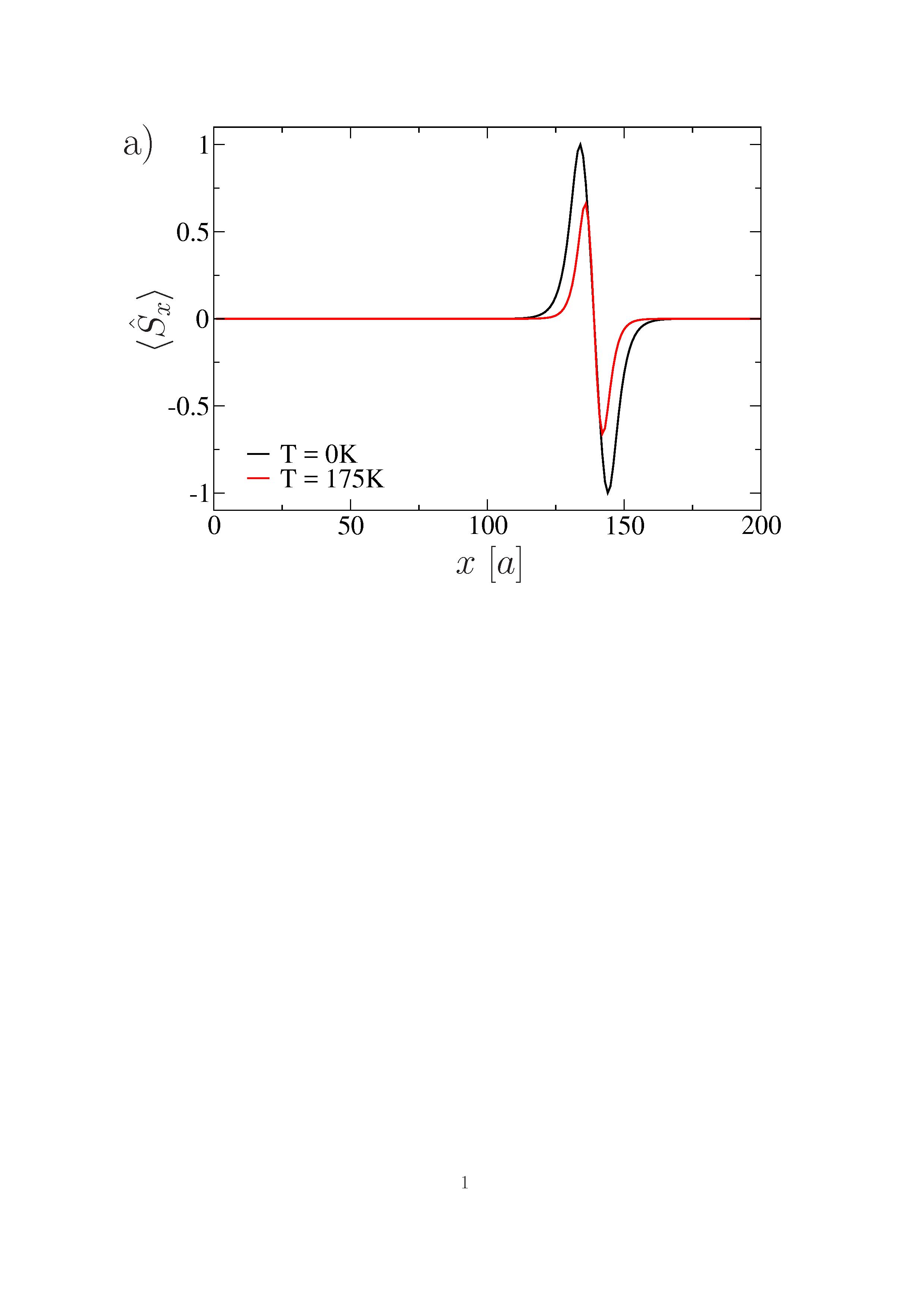
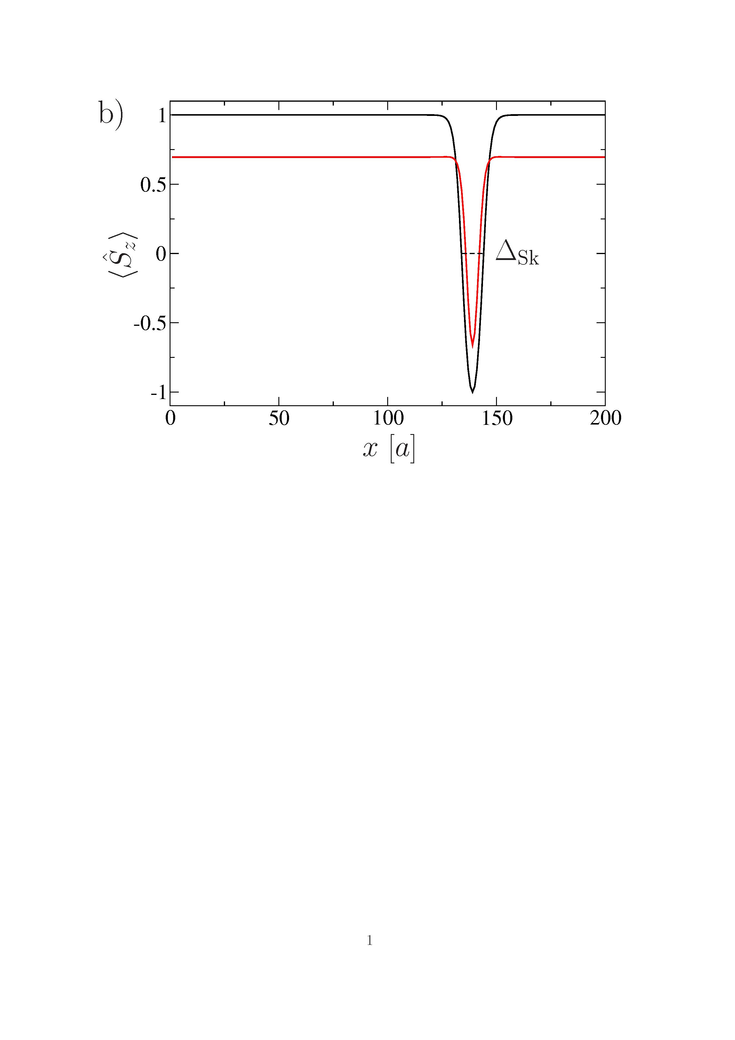
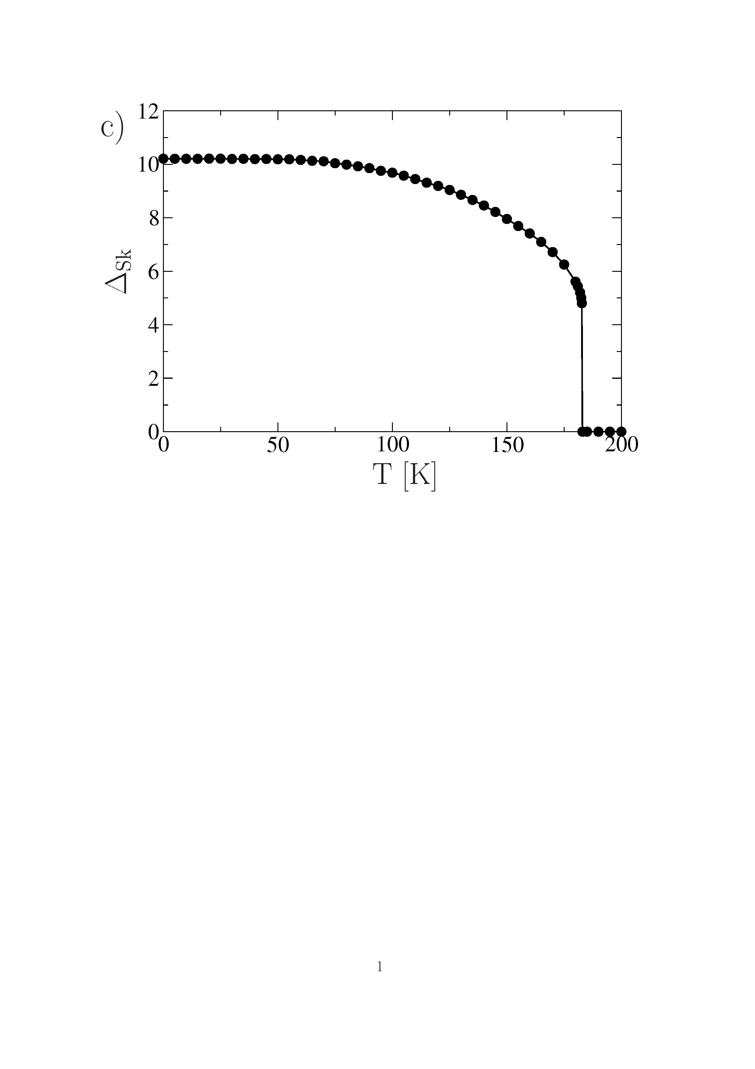
Figure 2: (color online) Magnetic Skyrmion temperature dependence: a) and b) Skyrmion profiles at $T=0$ K and $T=175$ K, c) Skyrmion width as function of temperature.

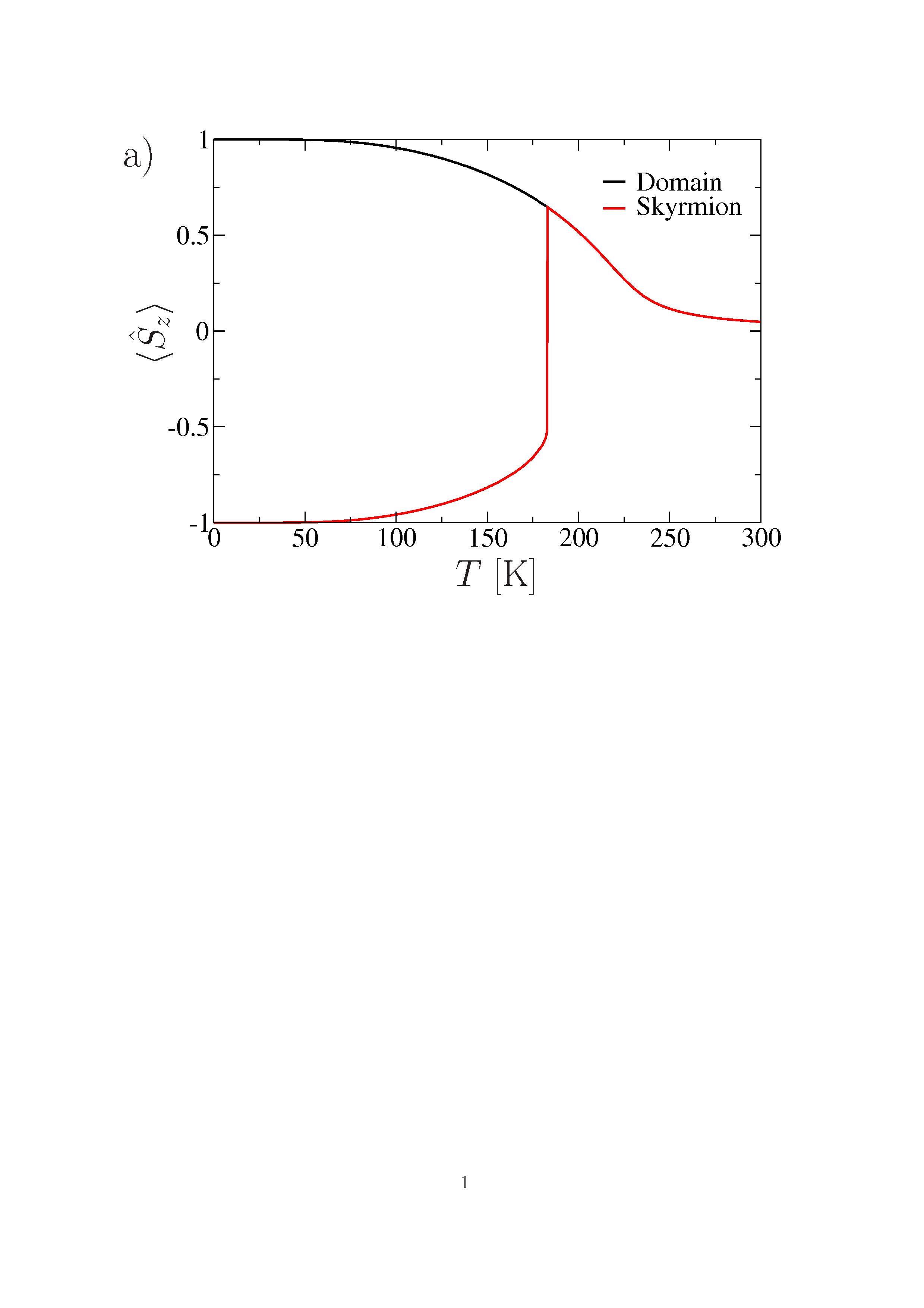
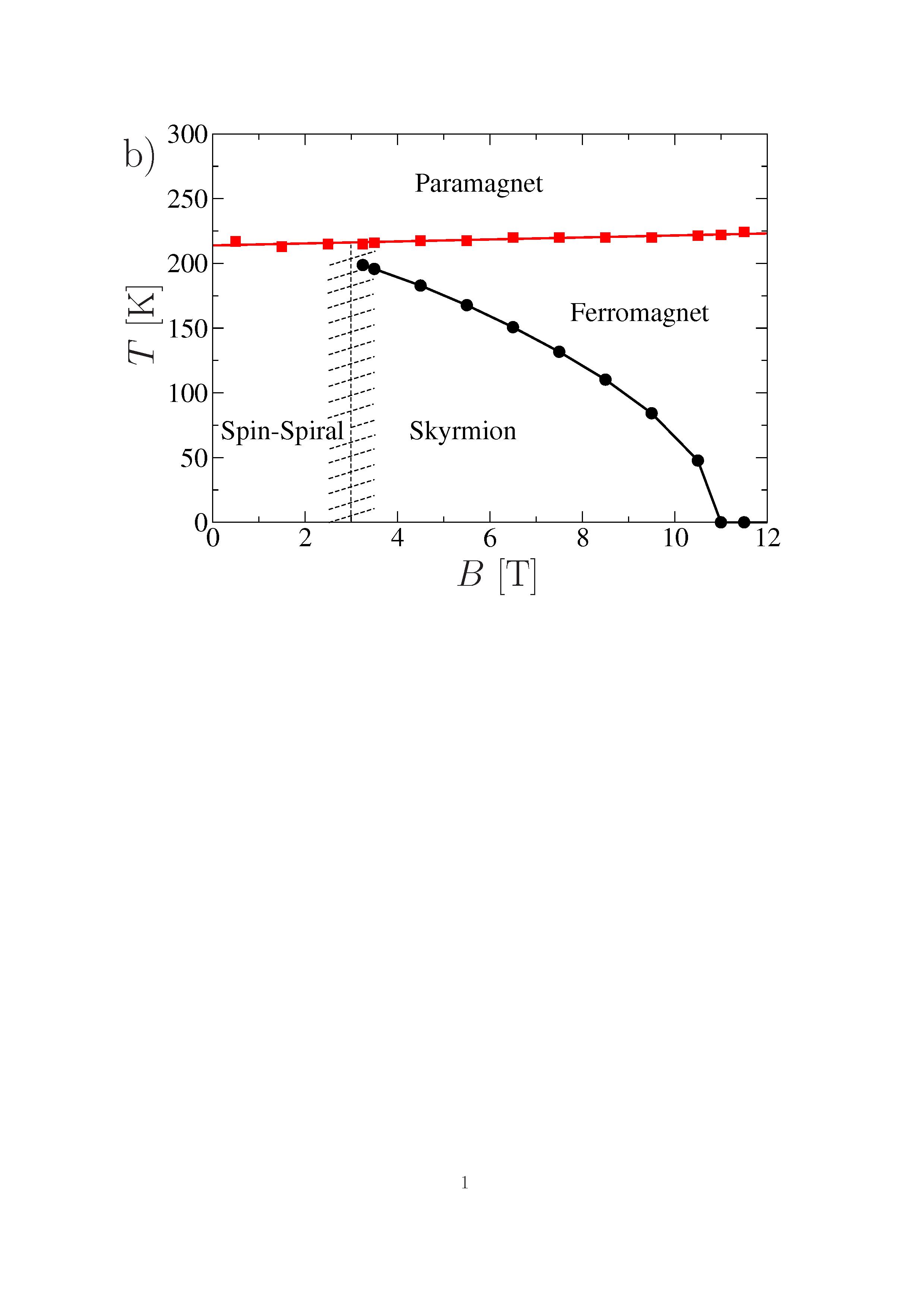
Figure 3: (color online) Temperature dependence: a) spin expectation values $\langle\hat{S}_{z}\rangle$ as function of temperature. The spin expectation values are calculated for the center of the Skyrmion and the surrounding domain. b) corresponding phase diagram with first (Skyrmion $\leftrightarrow$ Ferromagnet) and second order (Skyrmion / Ferromagnet $\leftrightarrow$ Paramagnet) phase transitions. The dashed area is the transition area between the Skyrmionic and the ferromagnetic phase. The pictures correspond to $B=4.5$ T.

With the definition of the effective field $\mathbf{B}_{n}^{\mathrm{eff}}=-\frac{\partial\hat{\mathrm{H}}}{\partial\hat{\mathbf{S}}_{n}}$, where $\mathbf{B}_{n}^{\mathrm{eff}}=(B_{n}^{x},B_{n}^{y},B_{n}^{z})^{T}$ is a real number, the Hamilton operator $\hat{\mathrm{H}}$ can be written as:

$$\hat{\mathrm{H}}=\sum\limits_{n}\mathbf{B}_{n}^{\mathrm{eff}}\cdot\hat{\mathbf{S}}_{n}\;.$$ (2)

Eq. (2) already shows the local character of the Hamiltonian.

Then, with the definition:

$$\hat{\mathrm{h}}_{n}=\mathbf{B}_{n}^{\mathrm{eff}}\cdot\hat{\mathbf{S}}_{n}\;,$$ (3)

$\hat{\mathrm{H}}$ can be finally written as sum of the local Hamilton operators $\hat{\mathrm{h}}_{n}$:

$$\hat{\mathrm{H}}=\sum\limits_{n}\hat{\mathrm{h}}_{n}\;.$$ (4)

III Thermodynamical studies

The temperature dependence of the ground state configuration of a spin system, like a magnetic Skyrmion, can be easily investigated. From statistical physics it is known that the spin expectation values are defined by:

$$\langle\hat{\mathbf{S}}_{n}\rangle=\frac{\mathrm{Tr}\left(\hat{\mathbf{S}}_{n}\exp(\beta\hat{\mathrm{H}})\right)}{\mathrm{Tr}\left(\exp(\beta\hat{\mathrm{H}})\right)}\;.$$ (5)

As usual $\beta$ is the inverse temperature: $\beta=\frac{1}{k_{B}T}$. In case of a quantum spin system the trace is the sum over all quantum numbers and therefore we find after some algebra an equation which can be easily solved numerical:

$$\langle\hat{\mathbf{S}}_{n}\rangle=g\mu_{B}{\cal B}_{S}(\beta B_{n}^{\mathrm{eff}})\;.$$ (6)

Within this equation ${\cal B}_{S}(\beta B_{n}^{\mathrm{eff}})$ is the Brillouin function:

$${\cal B}_{S}(\beta B_{n}^{\mathrm{eff}})=\frac{2S+1}{2S}\mathrm{coth}\left(\frac{2S+1}{2S}\beta B_{n}^{\mathrm{eff}}\right)-\frac{1}{2S}\mathrm{coth}\left(\frac{1}{2S}\beta B_{n}^{\mathrm{eff}}\right)\;.$$ (7)

Fig. 1 shows the Skyrmionic configuration at zero temperature ($T=0$ K) and $B=4.5$ T which can be derived by solving Eq. (6) self-consistent for a random initial configuration or a given Skyrmionic structure. Such a Skyrmion configuration can be found for $S=1$, but also for $S=1/2$ or in the case of a classical spin system ($S=\infty$). In Fig. 1a) the whole system ($z$-component of the spin expectation value $\langle\hat{\mathbf{S}}\rangle$) can be seen with a single Skyrmion located at $x=139$ $a$, $y=86$ $a$, where $a$ is the lattice constant of the system. Fig. 1b) provides the microscopic structure of the Skyrmion which due to the in plane DMI vectors is a Hedgehog structure, meaning all magnetic moments pointing to the center of the Skyrmion. Fig. 1c) and Fig. 1d) give the Skyrmion profiles which appear for a cut through the middle of the Skyrmion ($y=86$ $a=$ const.). Similar profiles can be found also using other simulation methods like Langevin spin dynamics García-Palacios and Lázaro (1998) or Monte Carlo simulations Hagemeister et al. (2015), but as already said the advantage of the SCF theory lays in the fact that temperature effects can be investigated without interfering noise. Fig. 2 shows the Skyrmion profiles for $T=0$ K and $T=175$ K. As expected the magnetization decreases with increasing temperature, but the profile of the Skyrmion does not changes even if the Skyrmion shrinks. The reduction of Skyrmion size with increasing temperature can be manifested with aid of the Skyrmion radius $\Delta_{\mathrm{Sk}}$. In the following, $\Delta_{\mathrm{Sk}}$ shall be defined as the distance between the two zero crossings of $\langle\hat{S}_{z}\rangle$ [see Fig. 2b)]. $\Delta_{\mathrm{Sk}}$ as function of temperature $T$ is given in Fig. 2c), $\Delta_{\mathrm{Sk}}$ decreases with increasing temperature and becomes zero at the critical temperature $T_{C}^{\mathrm{Sk}}=183$ K ($B_{z}=4.5$ T). Above this temperature the ferromagnetic state is the ground state, meaning $\Delta_{\mathrm{Sk}}=0$. The abrupt change of $\Delta_{\mathrm{Sk}}$ indicates that the transition is of first order which means that during the annihilation of the Skyrmion energy is released.

The first order phase transition can be observed also by investigating the local magnetization (spin expectation value $\langle\hat{S}_{n}^{z}\rangle$) as function of temperature $T$. More precisely the first order transition can be seen if the magnetization inside the Skyrmion is investigated. In the case of the surrounding ferromagnetic environment the phase transition is of second order. In Fig. 3a) the spin expectation values $\langle\hat{S}_{n}^{z}\rangle$ correspond to the center of the Skyrmion at $x=139$ $a$, $y=86$ $a$ and the surrounding ferromagnetic domain: $x=80$ $a$, $y=80$ $a$ are plotted as function of temperature. In both cases the absolute value $|\langle\hat{S}_{n}^{z}\rangle|$ are equal to one at zero temperature and decrease with increasing temperature. A careful analysis of the magnetization shows that inside the Skyrmion $|\langle\hat{S}_{n}^{z}\rangle|$ decreases faster than in the domain. In Fig. 3a) $\langle\hat{S}_{n}^{z}\rangle$ is plotted instead of $|\langle\hat{S}_{n}^{z}\rangle|$ to show the opposite orientation of $\langle\hat{S}_{n}^{z}\rangle$ inside the Skyrmion and the surrounding domain. The different temperature dependences of the magnetization inside and outside the Skyrmion are similar to the behavior of the magnetization of a magnetic Vortex Wieser et al. (2006) however with one significant difference. In the case of the Vortex the phase transitions of the magnetization of the Vortex core and the surrounding domain are both of second order and not of first and second order. Nevertheless, in both cases (Skyrmion and magnetic Vortex) we find two different critical temperatures $T_{C}^{\mathrm{Sk}}$ (Skyrmion) and $T_{C}^{\mathrm{FM}}$ (surrounding Ferromagnet): $T_{C}^{\mathrm{Sk}}=183$ K and $T_{C}^{\mathrm{FM}}=217.5$ K. Remark: These values correspond to an external magnetic field with $B_{z}=4.5$ T. In general $T_{C}^{\mathrm{Sk}}$ and $T_{C}^{\mathrm{FM}}$ depend on the external magnetic field. The dependence and therefore the phase diagram is given in Fig. 3b). As said before, the transition from the Skyrmion phase to the ferromagnetic phase is a first order phase transition and the phase transition from the ferromagnetic phase to the paramagnetic phase is of second order. Furthermore, there is another transition from the spin-spiral phase to the Skyrmion phase with increasing external field. The striped area marks the transition area where both phases coexist.

IV Eigenfunctions of $\hat{\mathrm{H}}$

Due to the fact that $\hat{\mathrm{H}}$ [Eq. (1)-(4)] is a quantum mechanical operator respectively mathematically a matrix it is possible to calculate the corresponding eigenvalues and eigenfunctions. In Sec. II it has been shown that the Hamiltonian $\hat{\mathrm{H}}$ can be written as sum of the local Hamilton operators $\hat{\mathrm{h}}_{n}$. Therefore, the problem reduces to calculate the eigenvalues $E_{n}$ and eigenvectors $\phi_{n}$ of $\hat{\mathrm{h}}_{n}$:

$$\hat{\mathrm{h}}_{n}{\boldsymbol{\phi}}_{n}=E_{n}{\boldsymbol{\phi}}_{n}\;.$$ (8)

Finally, the eigenvalues and eigenvectors or eigenfunctions of $\hat{\mathrm{H}}$ are the product states of $\phi_{n}$ respectively the sums over $E_{n}$.

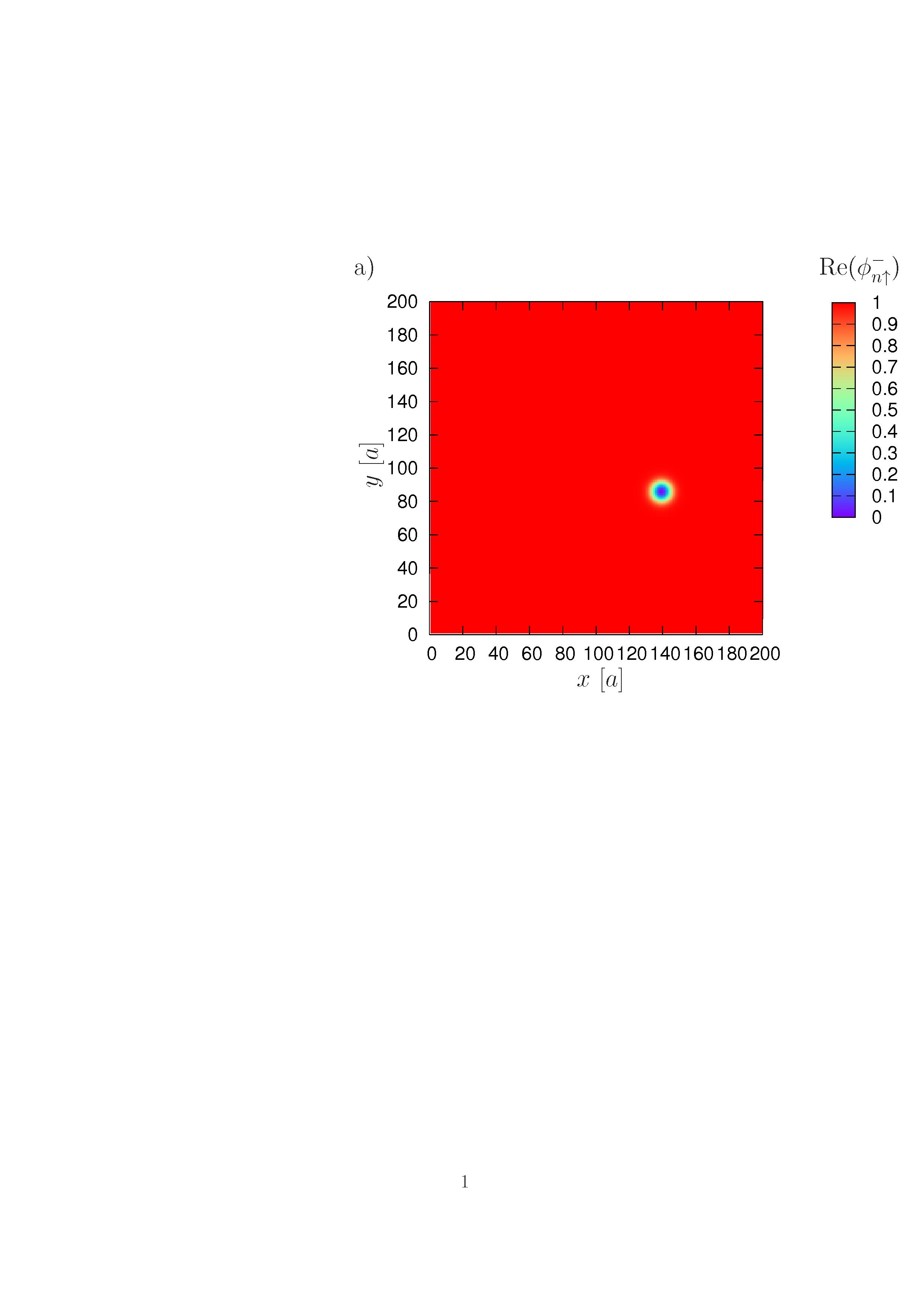
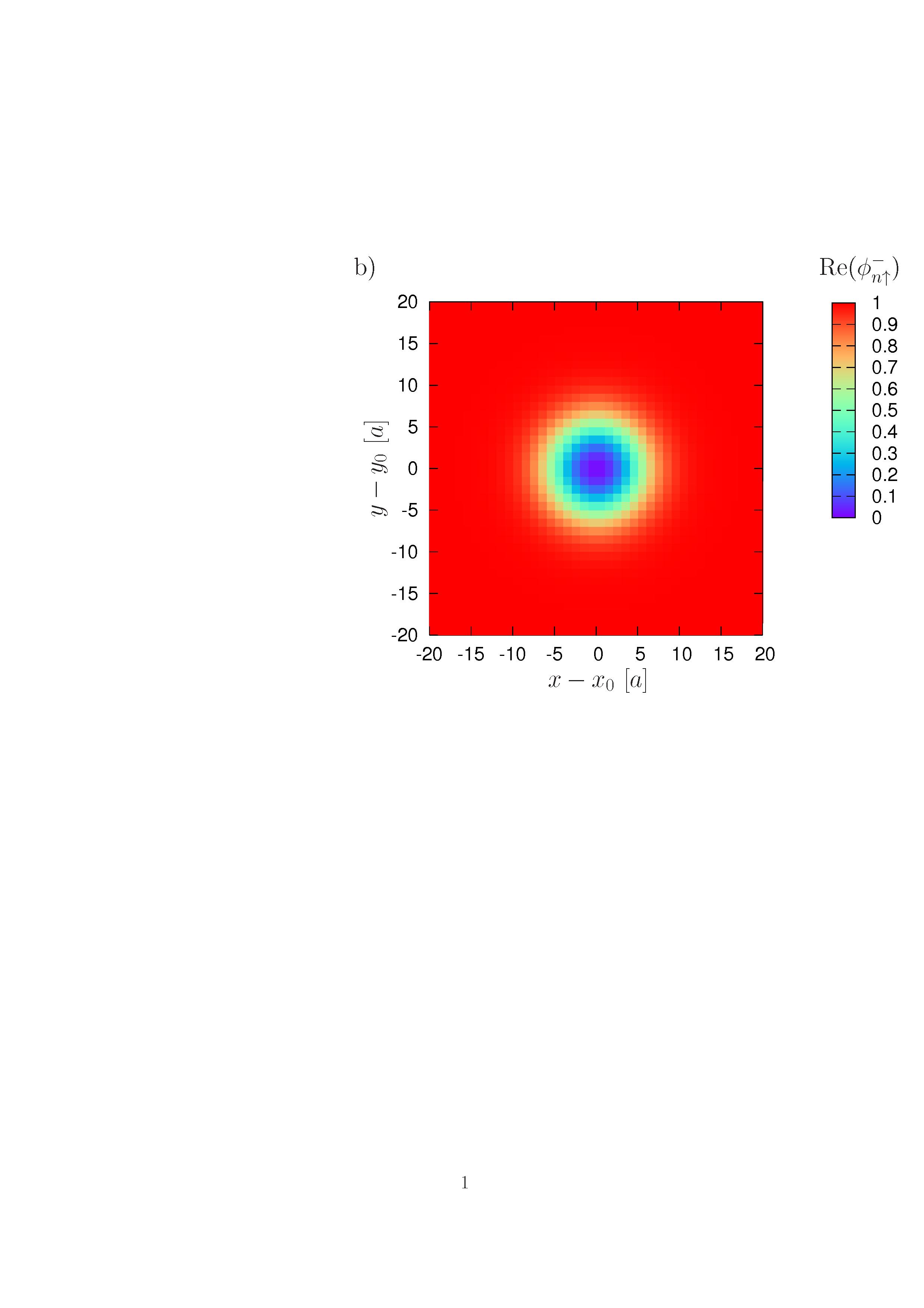
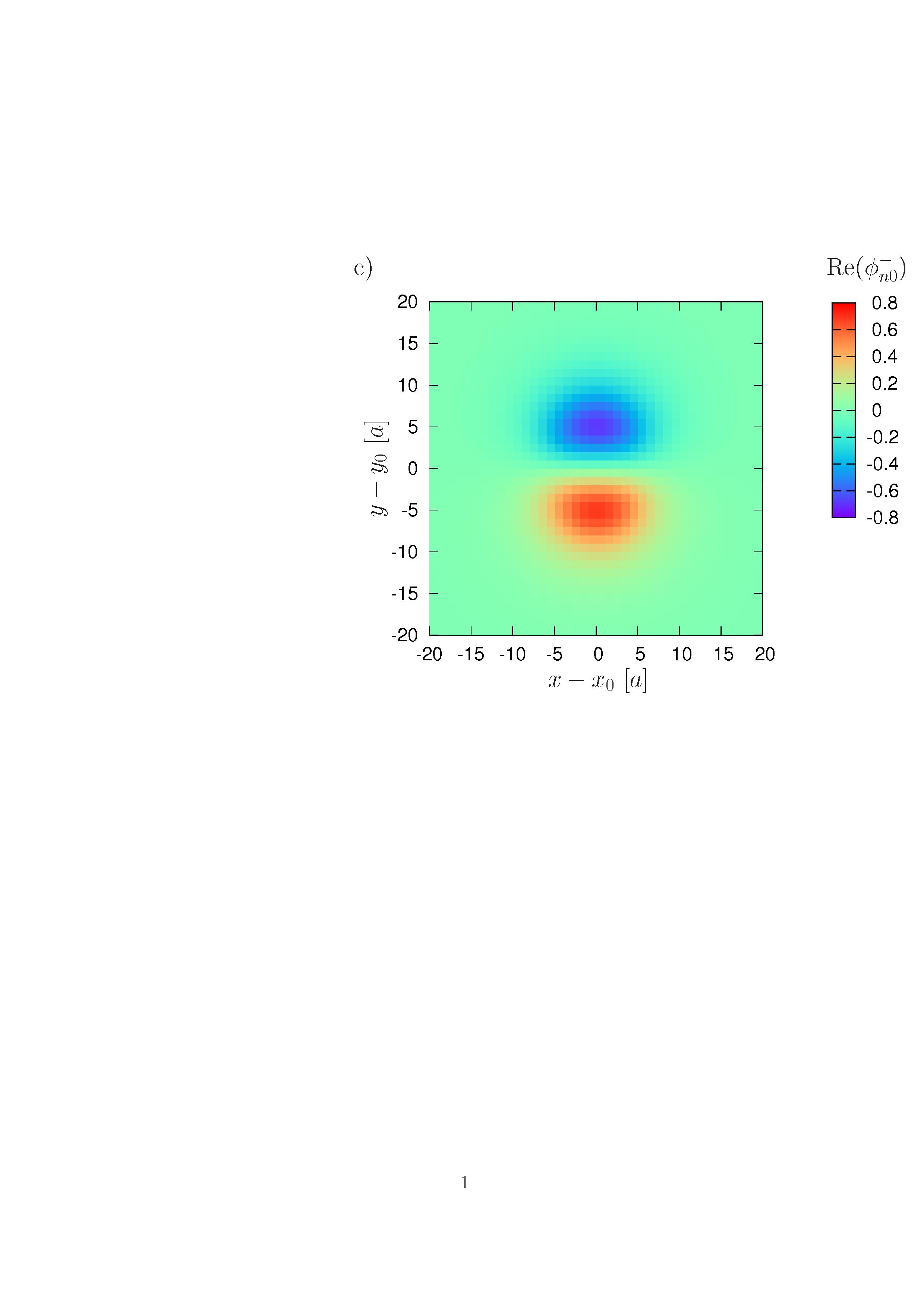
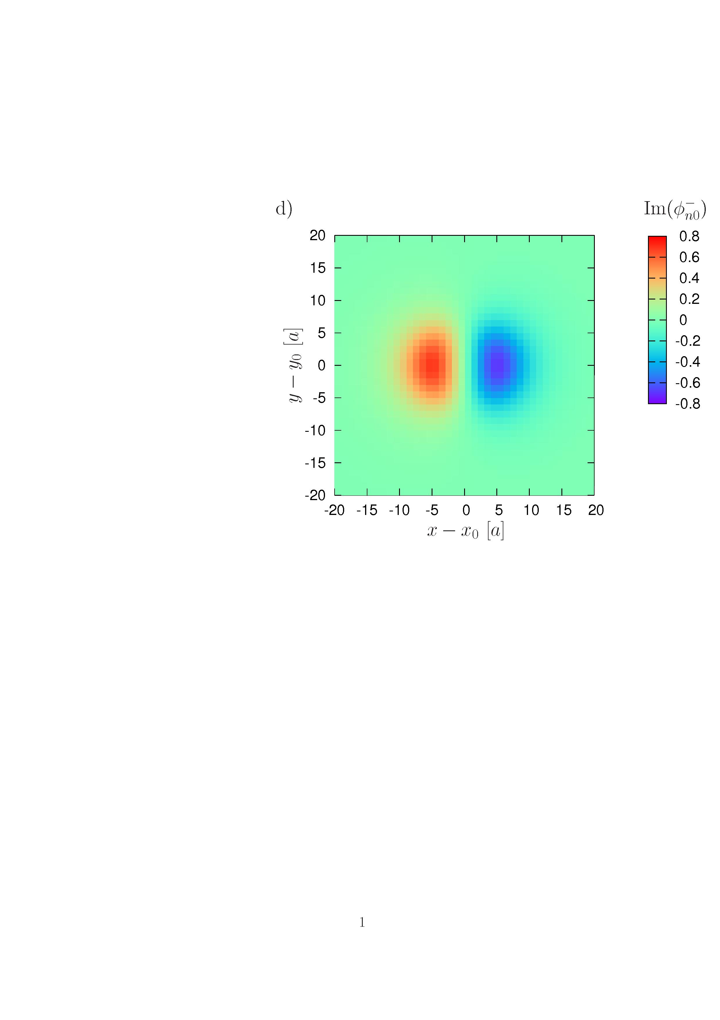
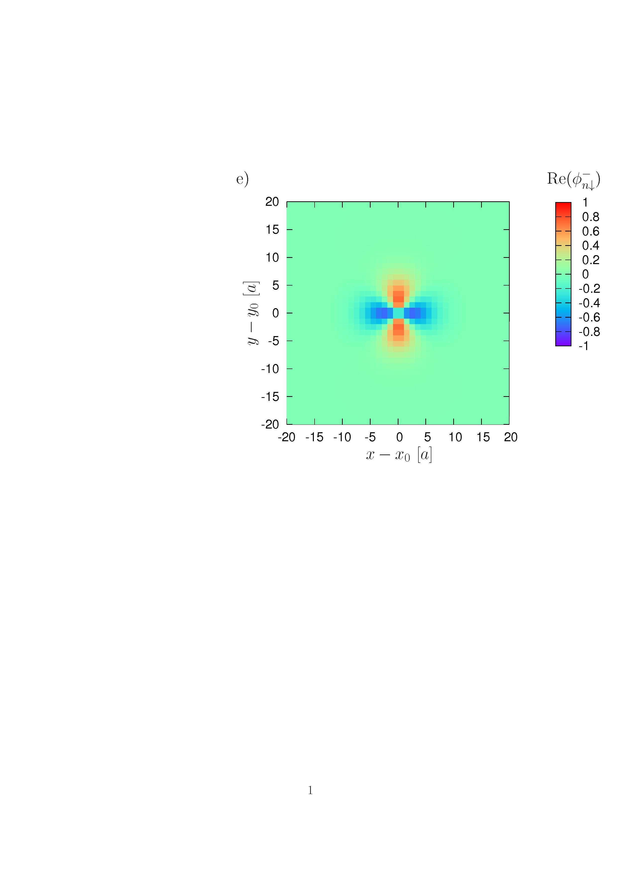
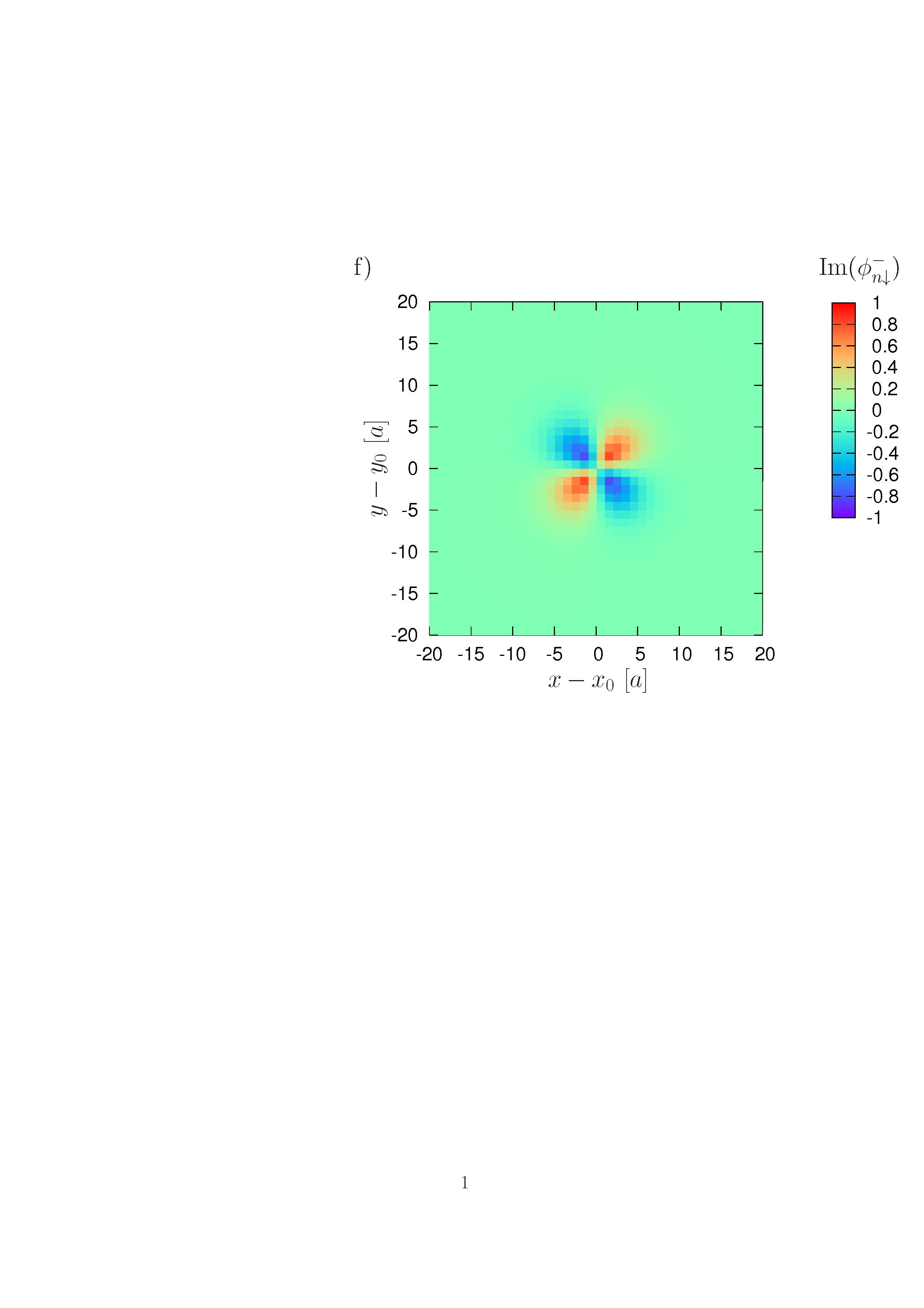
Figure 4: (color online) Eigenfunction of the ground state of a magnetic Skyrmion with $S=1$.

Mathematically, Eq. (8) is a matrix equation with the Hamilton operator $\hat{\mathrm{h}}_{n}$:

$$\hat{\mathrm{h}}_{n}=\left(\begin{array}[]{ccc}-B_{n}^{z}&\frac{-B_{n}^{x}+iB_{n}^{y}}{\sqrt{2}}&0\\ \frac{-B_{n}^{x}-iB_{n}^{y}}{\sqrt{2}}&0&\frac{-B_{n}^{x}+iB_{n}^{y}}{\sqrt{2}}\\ 0&\frac{-B_{n}^{x}-iB_{n}^{y}}{\sqrt{2}}&B_{n}^{z}\end{array}\right)$$ (12)

and the eigenvectors:

$${\boldsymbol{\phi}}_{n} = \left(\begin{array}[]{c}\phi_{n\uparrow}\\ \phi_{n0}\\ \phi_{n\downarrow}\end{array}\right)\;.$$ (16)

Using a standard diagonalization method the eigenenergies $E_{n}$ of $\hat{\mathrm{h}}_{n}$ are easily calculated:

$$E_{n}^{\pm} = \pm\mathrm{B}_{n}^{\mathrm{eff}}$$ (17)

$$E_{n}^{0} = 0\;.$$ (18)

Within Eq. (17) the effective fields $\mathrm{B}_{n}^{\mathrm{eff}}$ are given by:

$$\mathrm{B}_{n}^{\mathrm{eff}}=\sqrt{\left(B_{n}^{x}\right)^{2}+\left(B_{n}^{y}\right)^{2}+\left(B_{n}^{z}\right)^{2}}\;,$$ (19)

and the ground state is characterized by $E_{n}^{-}=-\mathrm{B}_{n}^{\mathrm{eff}}$, while the corresponding eigenvector is:

$${\boldsymbol{\phi}}_{n}^{-} = \left(\begin{array}[]{c}\frac{\mathrm{B}_{n}^{\mathrm{eff}}+B_{n}^{z}}{2\mathrm{B}_{n}^{\mathrm{eff}}}\\ \frac{\sqrt{2}}{2\mathrm{B}_{n}^{\mathrm{eff}}}\left(B_{n}^{x}+iB_{n}^{y}\right)\\ \left(\frac{\mathrm{B}_{n}^{\mathrm{eff}}-B_{n}^{z}}{2\mathrm{B}_{n}^{\mathrm{eff}}}\right)\!\!\!\left(\frac{B_{n}^{x}+iB_{n}^{y}}{B_{n}^{x}-iB_{n}^{y}}\right)\end{array}\right)\;.$$ (23)

Fig. 4 shows the real and imaginary parts of the vector components $\{\phi^{-}_{n\uparrow},\phi^{-}_{n0},\phi^{-}_{n\downarrow}\}\in\mathbb{C}$ of the eigenvector ${\boldsymbol{\phi}}^{-}_{n}$ corresponding to the Skyrmion shown in Fig. 1. Fig. 4a) provides the total system while Fig. 4b)-f) are zoomed into the area of the Skyrmion. In Fig. 4a), the Skyrmion is clearly visible as spot in the surrounding ferromagnetic environment which is characterized by ${\boldsymbol{\phi}}^{-}_{n}=(1,0,0)^{T}$, $n\not\in$. The Skyrmion itself is described by all three components $\phi^{-}_{n\uparrow}$, $\phi^{-}_{n0}$, and $\phi^{-}_{n\downarrow}$ of ${\boldsymbol{\phi}}^{-}_{n}$. Not shown in Fig. 4 is the imaginary part of $\phi^{-}_{n\uparrow}$ which has been set to zero during the calculation.

V Quantum spin dynamics

So far $\hat{\mathrm{H}}$ has been used to describe the thermodynamics of the magnetic Skyrmion. But, the Hamilton operator $\hat{\mathrm{H}}$ can also be used for the description of the spin dynamics of the Skyrmion. The underlying equation of motion is the time dependent Schrödinger equation with an additional damping term Wieser (2015):

$$i\hbar(1-\lambda^{2})\frac{\mathrm{d}}{\mathrm{d}t}|\Psi\rangle=\hat{\mathrm{H}}|\Psi\rangle-i\lambda(\hat{\mathrm{H}}-\langle\hat{\mathrm{H}}\rangle)|\Psi\rangle\;.$$ (24)

Within the Schrödinger equation $\lambda$ is a constant describing the strength of the energy dissipation ($\lambda\geq 0$). Furthermore, $\langle\hat{\mathrm{H}}\rangle=\langle\Psi|\hat{\mathrm{H}}|\Psi\rangle$, and $\hat{\mathrm{H}}$ given by Eq. (4).

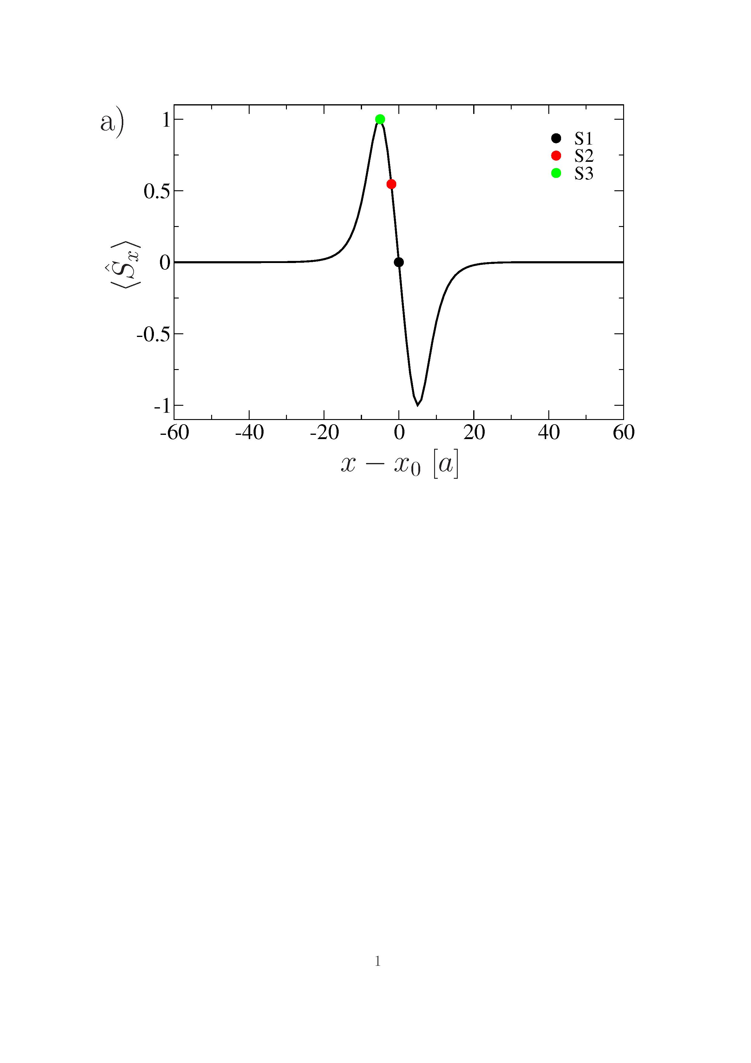
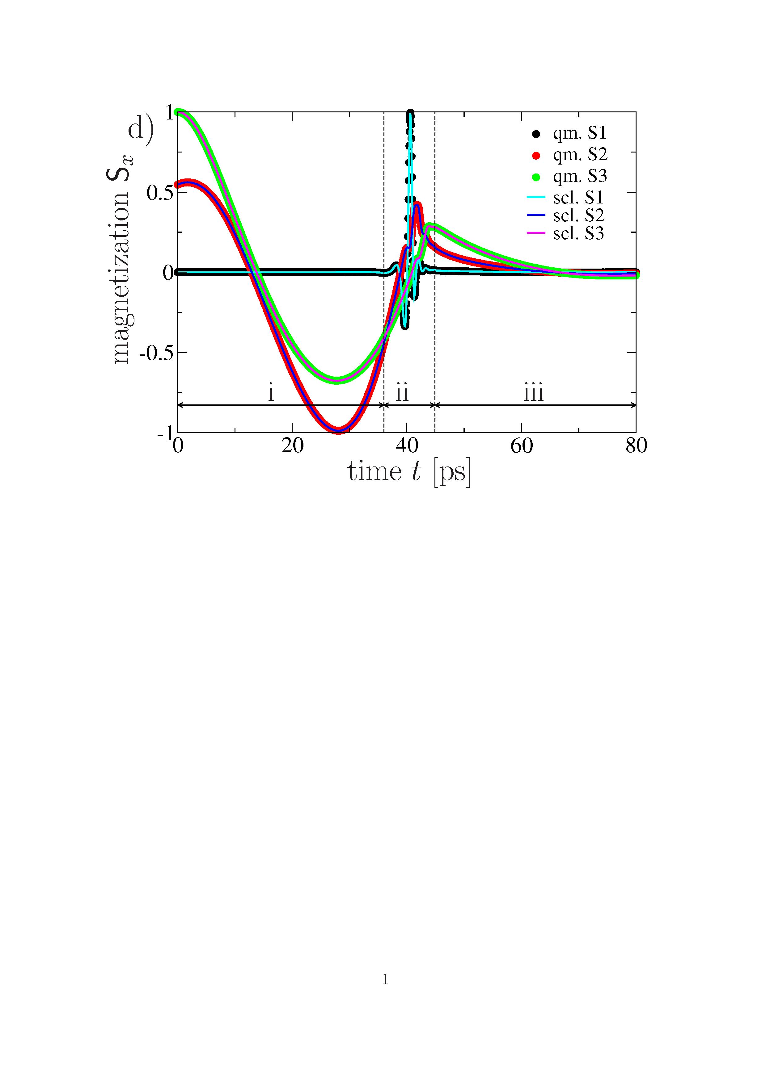
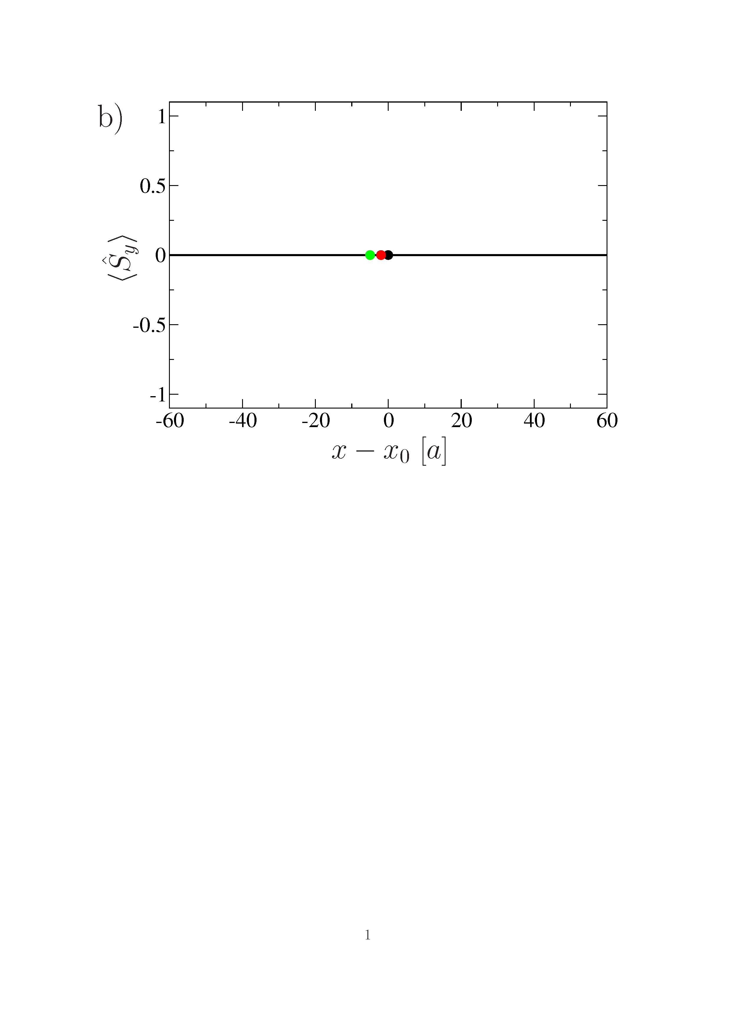
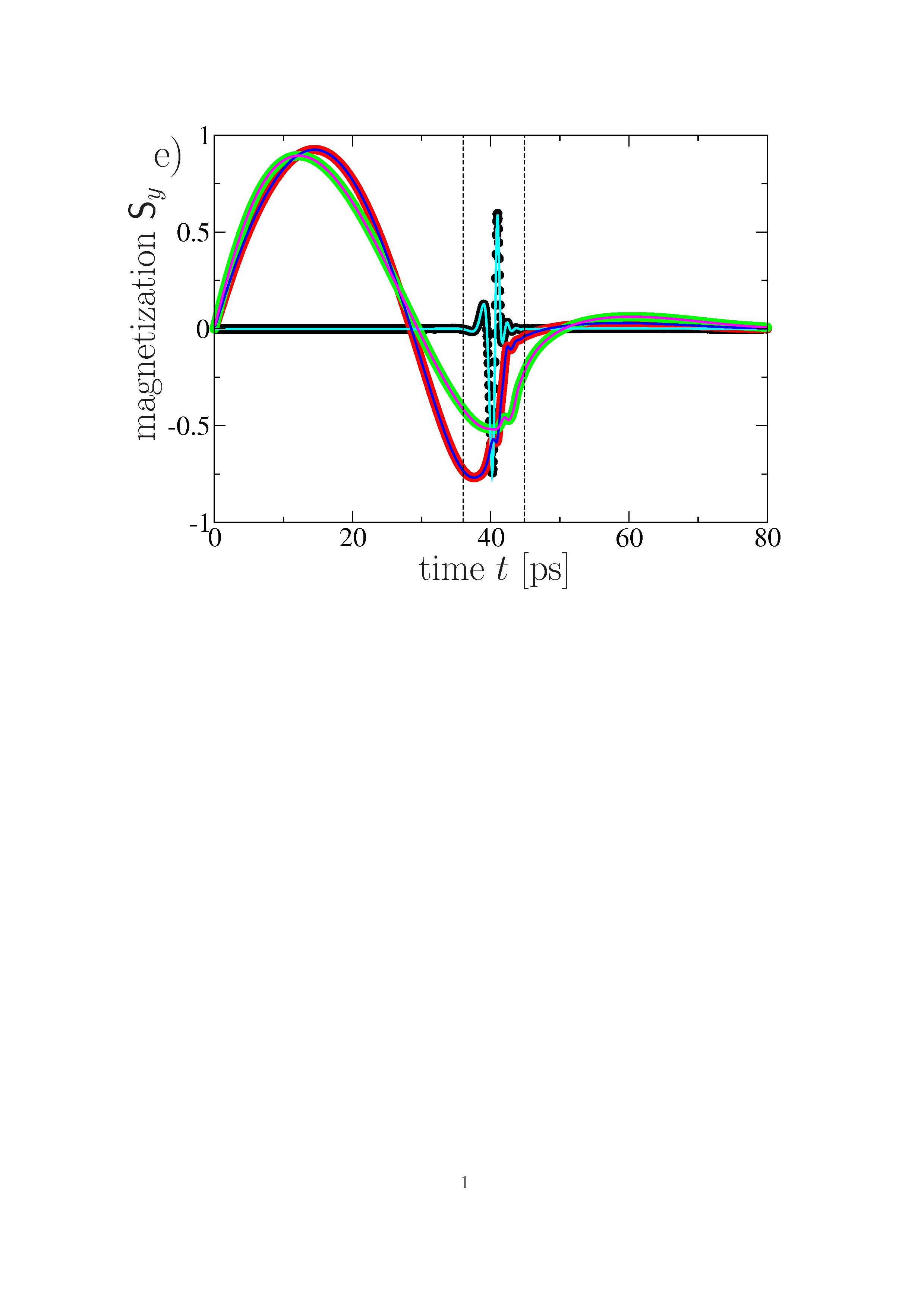
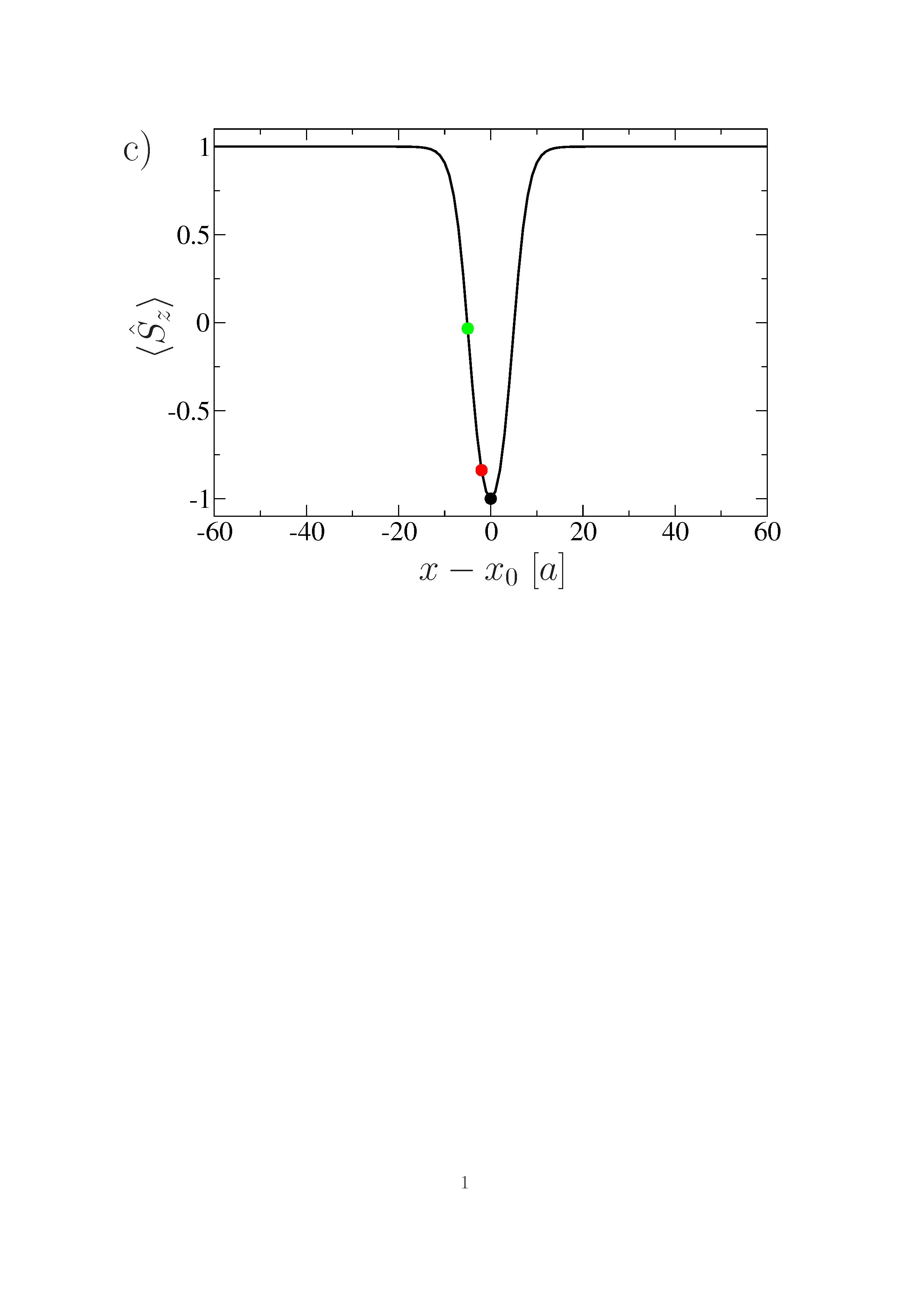
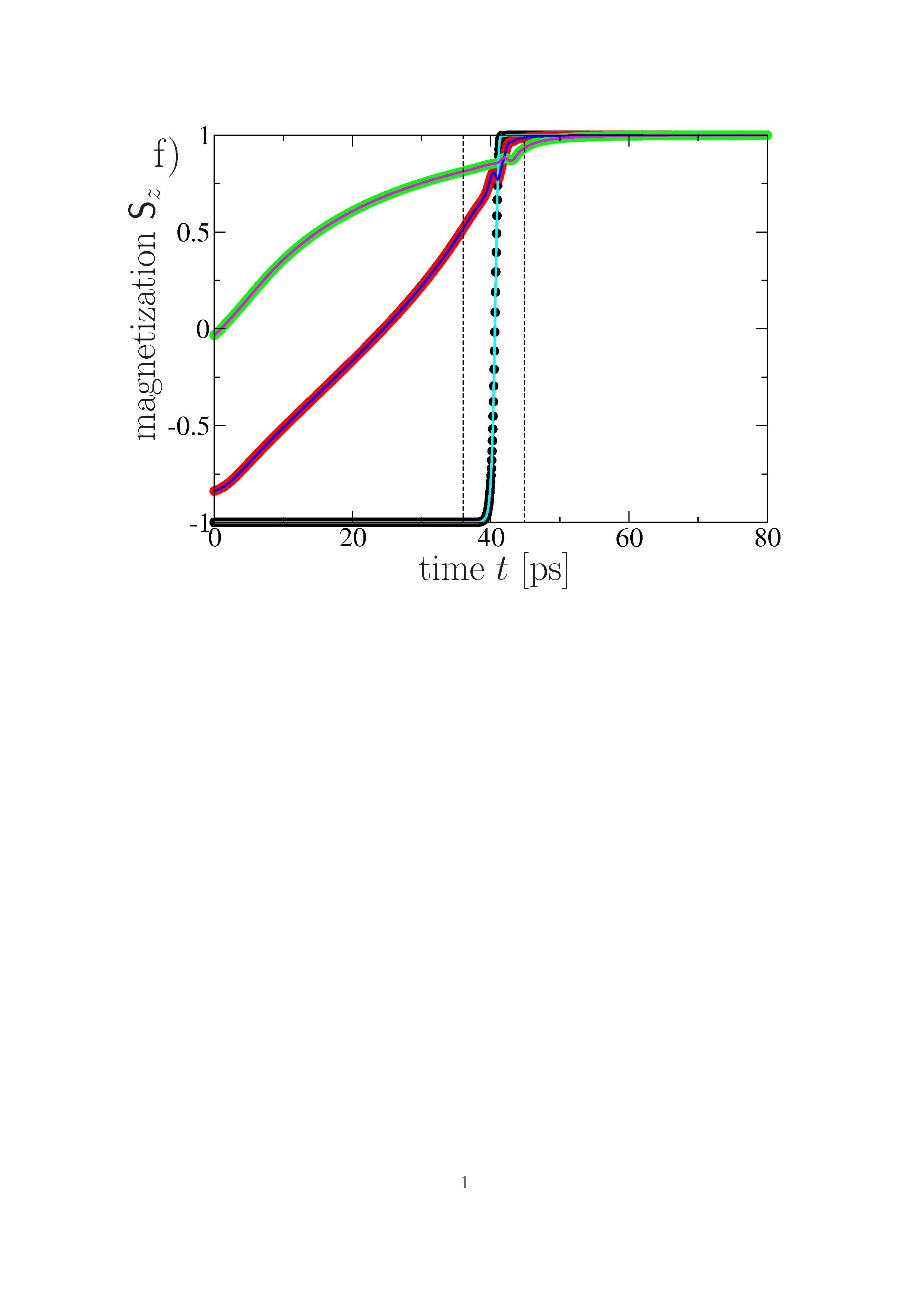
Figure 5: (color online) a), b), and c) Profiles of the magnetic Skyrmion calculated with aid of the time dependent Schrödinger Eq. (26). d), e), and f) trajectories of three spins S1-S3, marked as dots within the Skyrmion profiles, during the annihilation process forced by an electric field. The curves are calculated by solving the time dependent Schrödinger Eq. (26) (qm) as well as the semi-classical Eq. (V) (scl). The dynamics is divided into three phases i: shrinking, ii: collapse, and iii: shock wave.

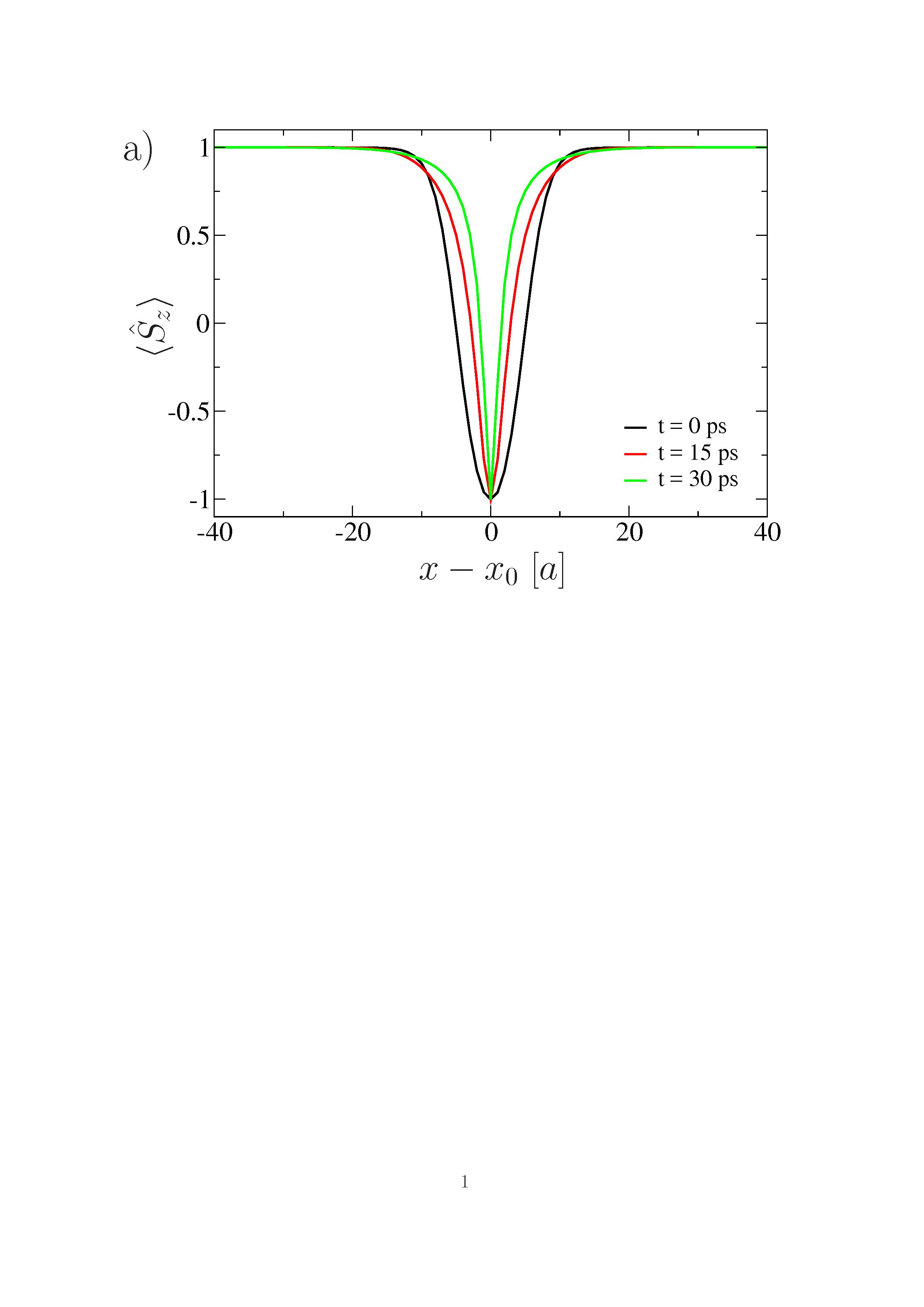
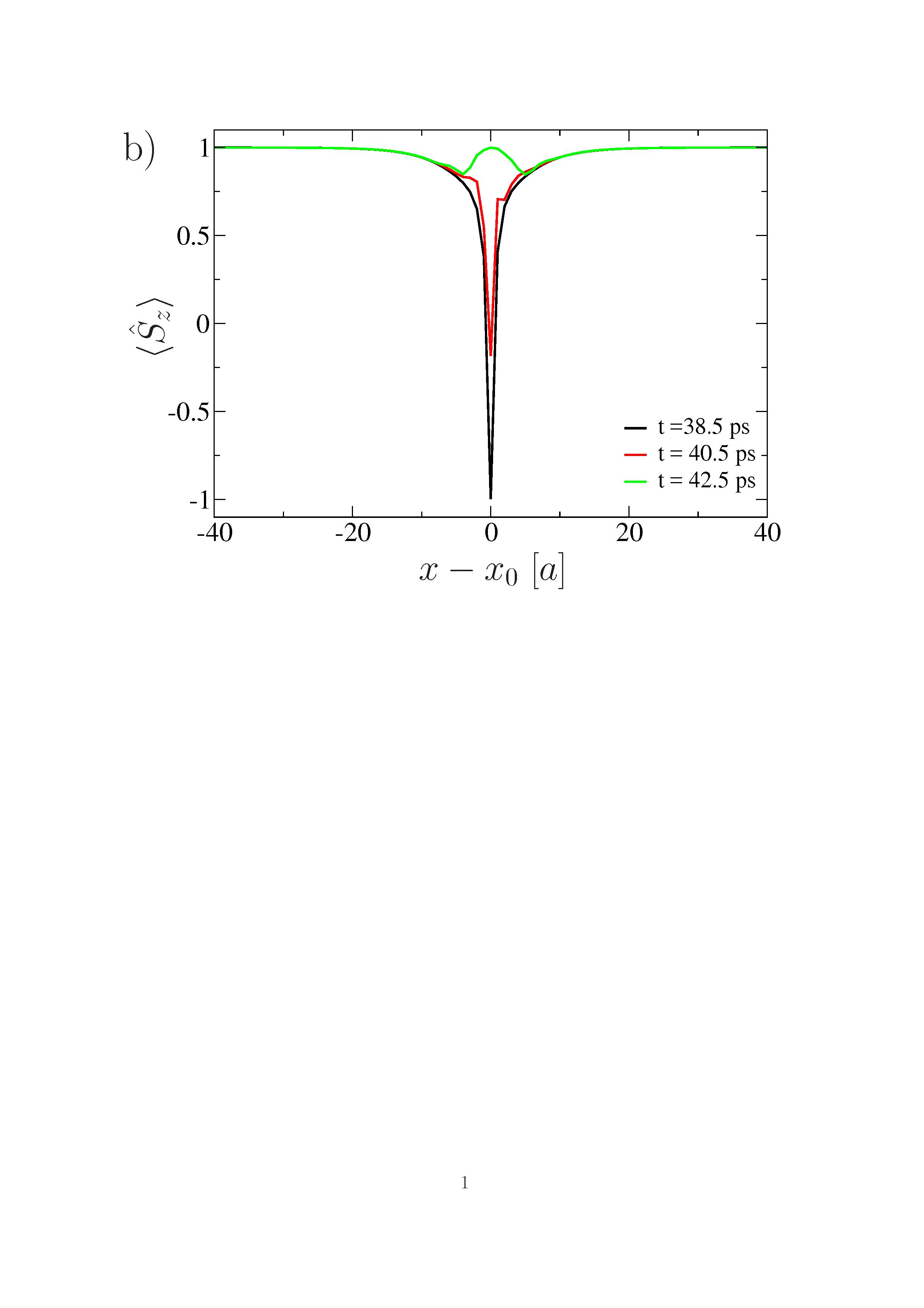
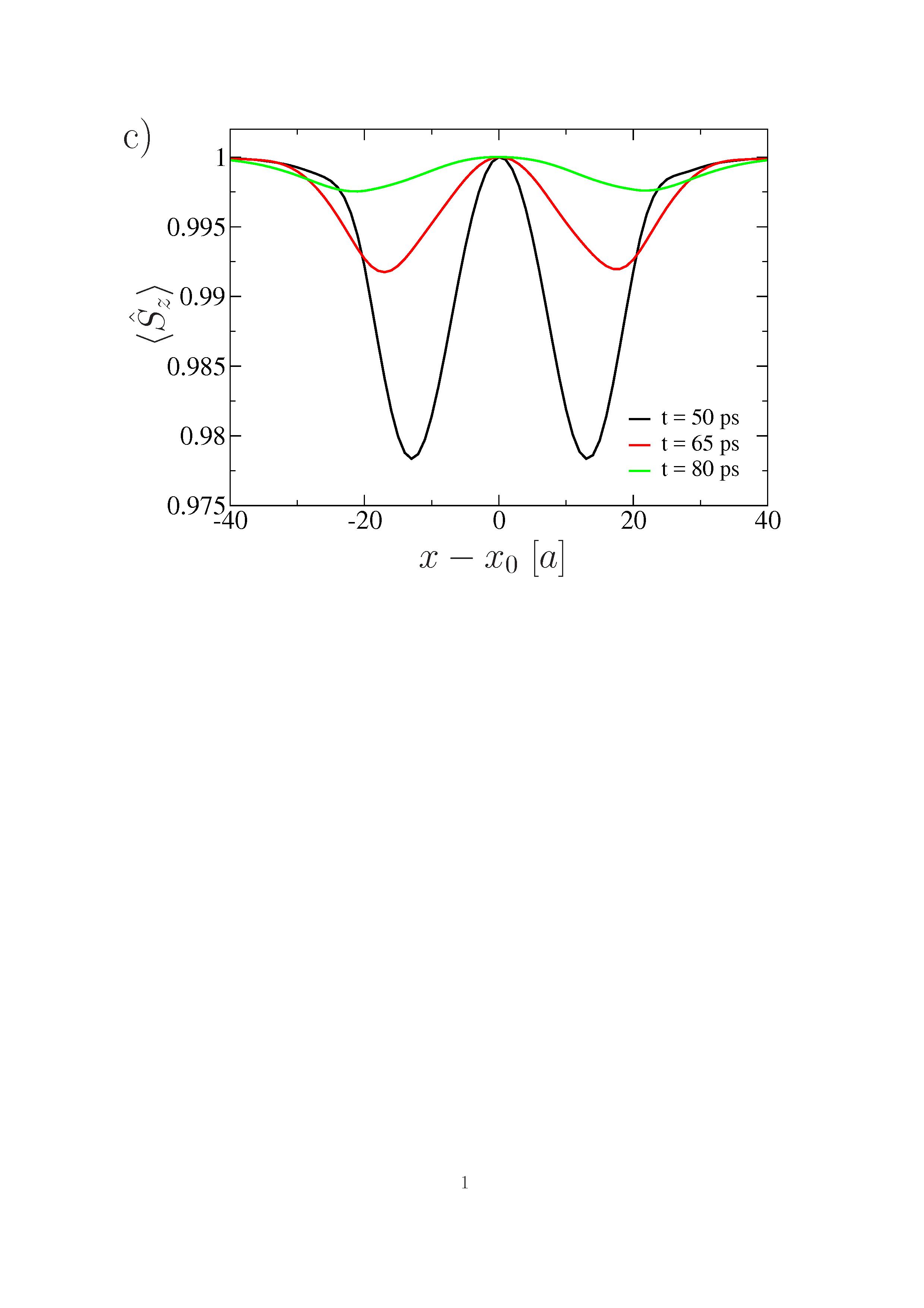
Figure 6: (color online) Skyrmion profiles during the electric field forced annihilation process:
a) phase i: shrinking, b) phase ii: collapse, and c) phase iii: shock wave.

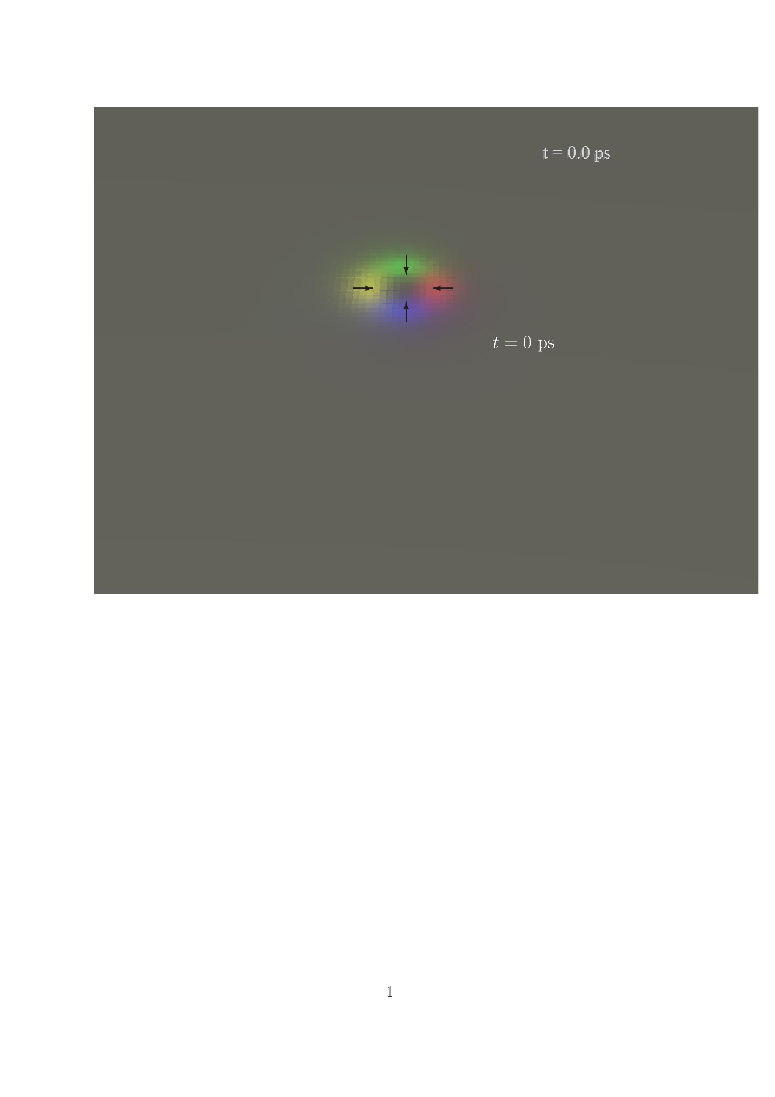
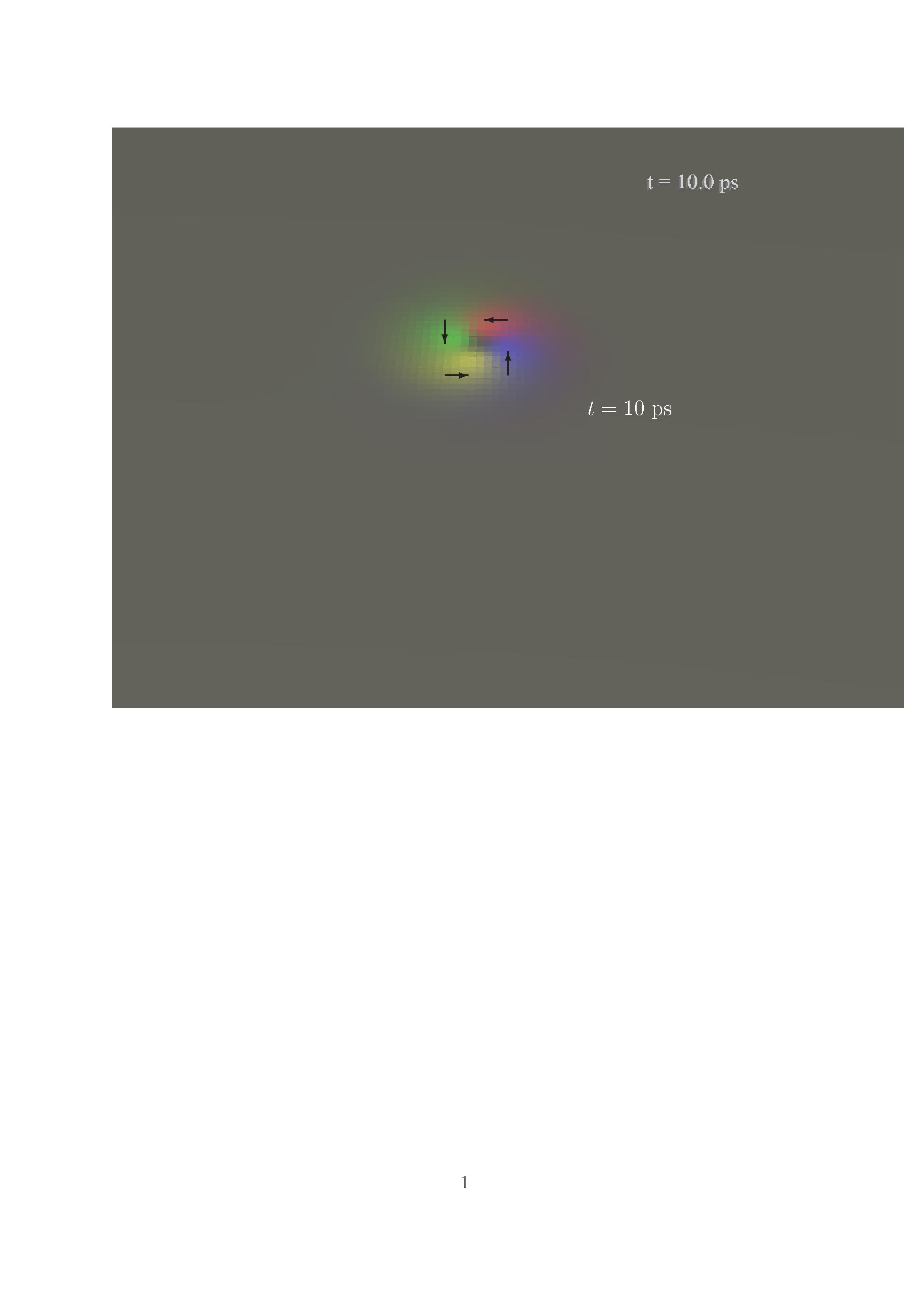
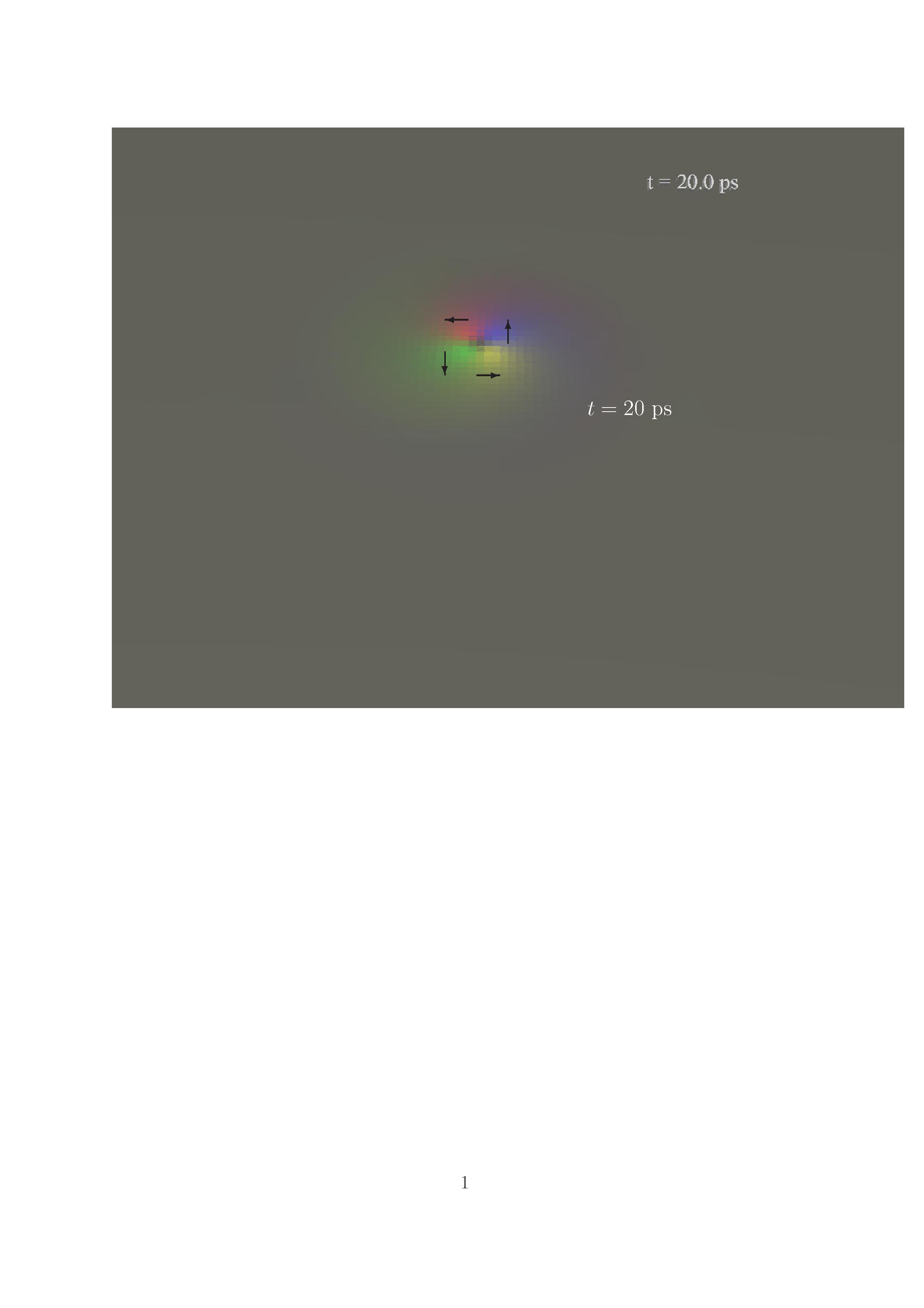
Figure 7: (color online) In-plane components of the magnetic Skyrmion during the annihilation process. The small arrows indicate the in-plane direction of the magnetization.

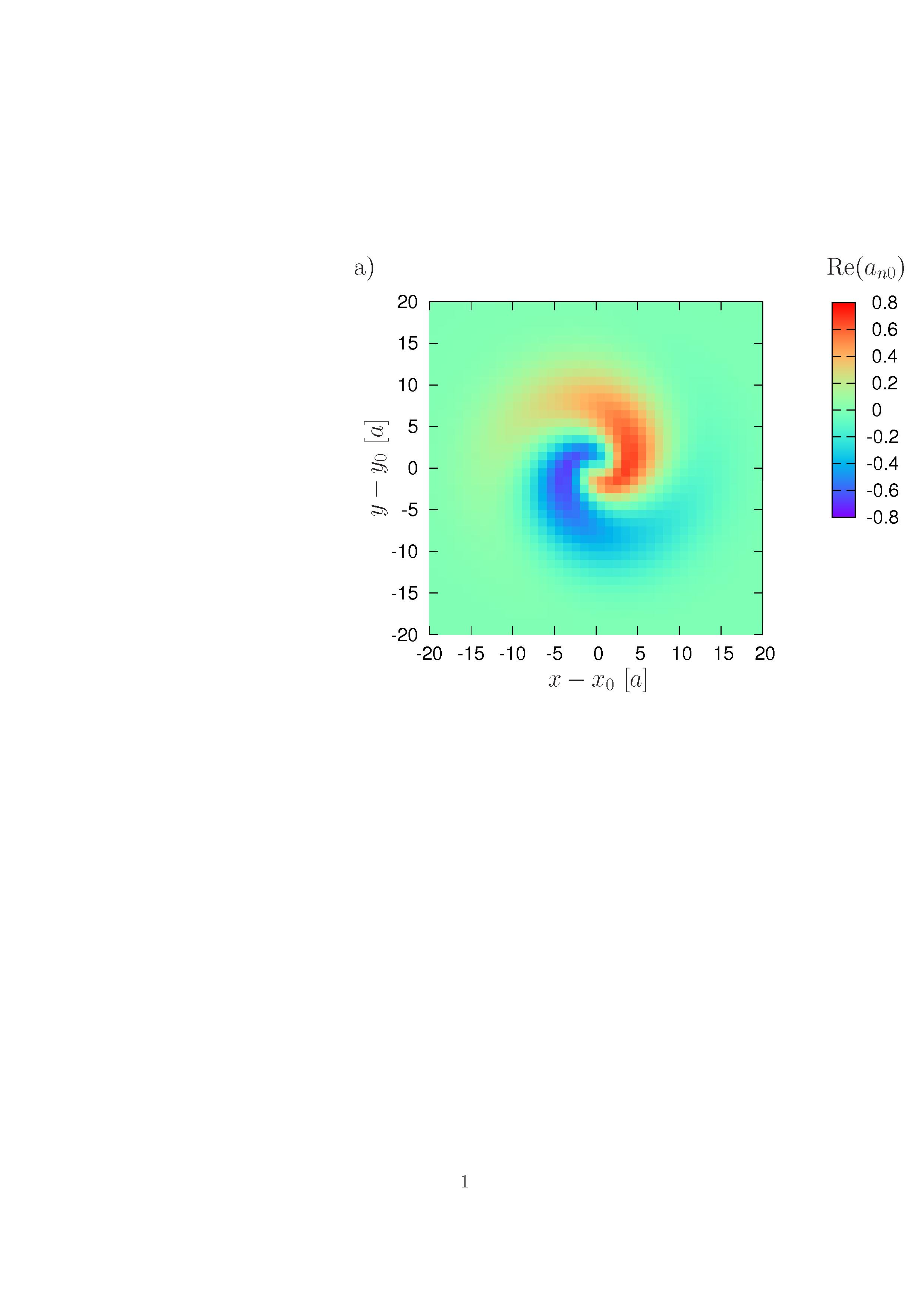
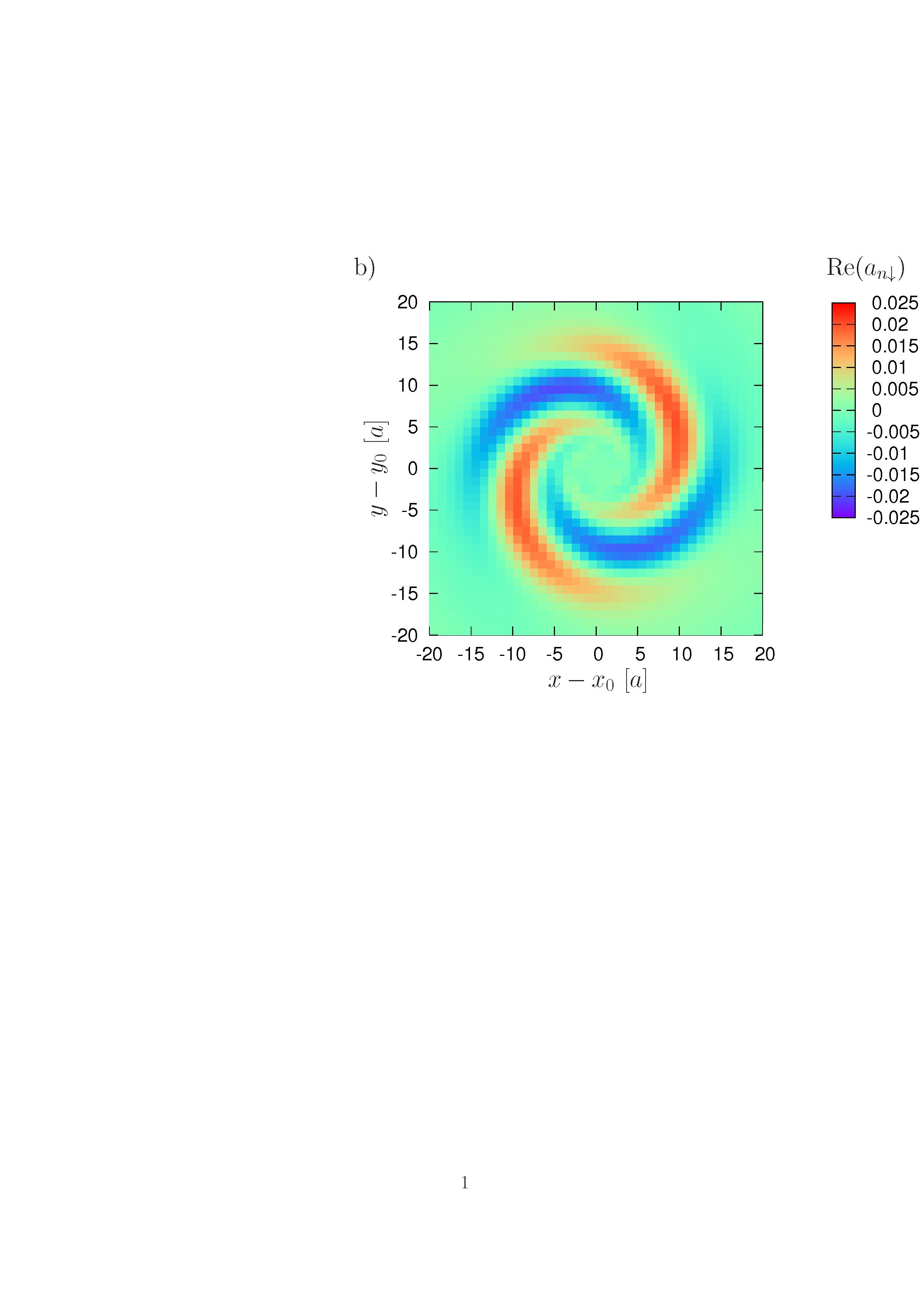
Figure 8: (color online) Real parts of the coefficients $a_{n0}$ and $a_{n\downarrow}$ of the wave functions $|\psi_{n}\rangle$ during the electric field forced Skyrmion annihilation. a) $\mathrm{Re}(a_{n0})$ at $t=10$ ps, b) $\mathrm{Re}(a_{n\downarrow})$ at $t=50$ ps.

Due to the fact that the Hamilton operator $\hat{\mathrm{H}}$ can be written as sum of the local Hamilton operators $\hat{\mathrm{h}}_{n}$ the wave function $|\Psi\rangle$ is a product state of the local wave functions $|\psi_{n}\rangle$:

$$|\Psi\rangle=\bigotimes\limits_{n=1}^{N}|\psi_{n}\rangle\;,$$ (25)

where $N=200\times 200=40000$. With Eq. (4) and Eq. (25) the time dependent Schrödinger equation becomes a set of coupled differential equations:

$$i\hbar(1-\lambda^{2})\frac{\mathrm{d}}{\mathrm{d}t}|\psi_{n}\rangle=\hat{\mathrm{h}}_{n}|\psi_{n}\rangle-i\lambda(\hat{\mathrm{h}}_{n}-\langle\hat{\mathrm{h}}_{n}\rangle)|\psi_{n}\rangle\;,$$ (26)

where $\langle\hat{\mathrm{h}}_{n}\rangle=\langle\psi_{n}|\hat{\mathrm{h}}_{n}|\psi_{n}\rangle$. The wave functions $|\psi_{n}\rangle$ can be constructed with aid of the Zeeman basis Edén (2003) where the basis vectors are $|j\rangle\in\{|\!\uparrow\rangle,|0\rangle,|\!\downarrow\rangle\}$:

$$|\psi_{n}\rangle=\sum_{j}a_{nj}|j\rangle\;.$$ (27)

In case the system is in the ground state the coefficients $a_{nj}$ are equal to $\phi^{-}_{nj}$ and the wave functions $|\psi_{n}\rangle$ are equal to the eigenvectors ${\boldsymbol{\phi}}_{n}^{-}$ (see Sec. IV). Due the fact that the wave function $|\Psi\rangle$ is a product state [see Eq. (25)] the system shows no entanglement. Therefore we can expect a spin dynamics which is similar to the dynamics provided by a description using classical spins Wieser (2016a).

In general the interest in the wave functions $|\psi_{n}\rangle$ is restricted despite the fact that the wave functions can provide additional information about the quantum system. More important and necessary for the dynamics are the spin expectation values:

$$\langle\hat{\mathbf{S}}_{n}\rangle=\langle\Psi|\hat{\mathbf{S}}_{n}|\Psi\rangle=\langle\psi_{n}|\hat{\mathbf{S}}_{n}|\psi_{n}\rangle\;.$$ (28)

In the previous publications Wieser (2015, 2016a) it has been shown that without entanglement the dynamics of the spin expectation values are well described by the following differential equation:

$$(1-\lambda^{2})\frac{\mathrm{d}}{\mathrm{d}t}\langle\hat{\mathbf{S}}_{n}\rangle=\gamma\langle\hat{\mathbf{S}}_{n}\rangle\times(\mathbf{B}_{n}^{\mathrm{eff}}-\lambda(\langle\hat{\mathbf{S}}_{n}\rangle\times\mathbf{B}_{n}^{\mathrm{eff}}))\;,$$

where $\gamma=g\mu_{B}/\hbar$ is the gyromagnetic ratio. The important point here is that due to the absence of entanglement the absolute values $|\langle\hat{\mathbf{S}}_{n}\rangle|=\hbar S$ are time independent (constant). The spin expectation values $\langle\hat{\mathbf{S}}_{n}\rangle$ only change their orientations in spin space. This is similar to the dynamics of the classical spins $\mathbf{S}_{n}$ described by the Landau-Lifshitz-Gilbert (LLG) equation. Indeed, Eq. (V) is identical to the LLG equation just with a tiny difference: the sense of rotation of the precession is reversed (for details see Wieser (2016a)).

Fig. 5 shows the trajectories of three spins during the annihilation of a Skyrmion due to the external electric field. Hsu et al. Hsu et al. (2016) have demonstrated that it is possible to use a local electric field generated by a scanning tunneling microscope to create or annihilate magnetic Skyrmions. However, the theoretical explanation for this phenomenon is is missing within the publication of Hsu et al. which is the tuning of the Dzyaloshinsky Moriya interaction by the electric field Wieser (2016b):

$${\boldsymbol{\cal D}}_{nm}={\boldsymbol{\cal D}}_{nm}^{0}+{\boldsymbol{\omega}}_{nm}(\mathbf{E}\times\mathbf{r}_{nm})\;.$$ (30)

Within this formula the ${\boldsymbol{\cal D}}_{nm}$ are the Dzyaloshinsky Moriya vectors after modification due to the electric field $\mathbf{E}$. The original Dzyaloshinsky Moriya vectors are ${\boldsymbol{\cal D}}_{nm}^{0}$ while $\mathbf{r}_{nm}$ is the vector pointing from lattice site $m$ to lattice site $n$. The prefactor ${\boldsymbol{\omega}}_{nm}$ is a constant which describes the strength of the modification due to the electric field. In the case of the experiment using the scanning tunneling microscope the modification of the Dzyaloshinsky Moriya vectors is local underneath the scanning tunneling microscope tip and the electric field vector $\mathbf{E}$ perpendicular to $\mathbf{r}_{nm}$. Depending on the orientation and strength of $\mathbf{E}$ the Dzyaloshinsky Moriya interaction becomes increased or reduced. Within the spin dynamics simulations presented in the following a constant modification ${\boldsymbol{\omega}}_{nm}=$ const. within a radius of $20$ lattice sites is assumed in such a way that outside this circle the strength of the Dzyaloshinsky Moriya interaction is not modified ${\boldsymbol{\omega}}_{nm}=0$ while inside the circle the Dzyaloshinsky Moriya interaction is zero ${\boldsymbol{\cal D}}_{nm}=0$. This modification simulates the influence of the electric field provided by the scanning tunneling microscope tip in the experiment by Hsu et al.. Thereby, the field vector $\mathbf{E}$ is perpendicular to the film plane $\mathbf{E}\perp\mathbf{r}_{nm}$ pointing to the film plane. Without Dzyaloshinsky Moriya interaction the ferromagnetic state is the ground state and the Skyrmion gets annihilated. Additional, within the spin dynamics simulation a small misalignment of the center of the Skyrmion and the magnetic tip (center of the circle) $0.5$ lattice constants in both directions $x$ and $y$ has been assumed. The small misalignment has the reason to break the symmetry of the central spin which otherwise would have no distinguished spin torque during the annihilation process. During the experiment by Hsu et al. the symmetry is broken either by thermal fluctuations or by also by misalignment respectively assymmetry of the electric field due to an non-symmetric tip. Fig. 5 provides the trajectories of the three spins mentioned before. The spins are marked by the colored dots in Fig. 5a)-c), where Fig. 5a) provides the Skyrmion profile corresponding to the $x$-component, Fig. 5b) the $y$-component, and Fig. 5c) the $z$-component of the spin expectation value $\langle\hat{\mathbf{S}}_{n}\rangle$. The trajectories in Fig. 5d)-f) are calculated in two ways: 1. solving the time dependent Schrödinger Eq. (26) and 2. solving the semi-classical differential Eq. (V). The remarkable fact is that the trajectories of both calculations show a perfect agreement. At this point it is necessary to mention that the agreement is a consequence of the absent entanglement.

Now the question is what are the advantages and disadvantages of using the semi-classical differential Eq. (V) instead of solving the time dependent Schrödinger equation? The advantage of the semi-classical differential equation is the fact that we have to calculate only three (one for $\langle\hat{S}_{n}^{x}\rangle$, $\langle\hat{S}_{n}^{y}\rangle$, and $\langle\hat{S}_{n}^{z}\rangle$) instead of six (real and imaginary part of $a_{n\uparrow},a_{n0},a_{n\downarrow}$) differential equations per lattice site. Furthermore, the spin expectation values $\langle\hat{\mathbf{S}}_{n}\rangle$ are directly given while for the time dependent Schrödinger equation first the wave functions $|\psi_{n}\rangle$ have to be calculated and in a second step the expectation values $\langle\hat{S}_{n}^{\eta}\rangle$, $\eta\in\{x,y,z\}$. Therefore, it can be said that in summary the effort and also the possible numerical errors are reduced by using the semi-classical differential Eq. (V) instead of the time dependent Schrödinger Eq. (26). However, on the other hand, Eq. (V) does not provide the wave functions $|\psi_{n}\rangle$. This means that the information, delivered by the wave functions, get lost. Furthermore, in the case of entanglement it is necessary to solve the time dependent Schrödinger equation.

So far we got a rough idea about the annihilation process provided by Fig. 5. The process itself can be divided into three phases marked by the roman numbers: The first phase (phase i) is characterized by the shrinking of the Skyrmion. During the second phase (phase ii) the Skyrmion collapses. And the third phase (phase iii) is a shock wave running trough the system. Corresponding to this dynamics Fig. 6 shows the profile of the Skyrmion during these three phases: Fig. 6a) corresponds to phase i, Fig. 6b) to phase ii and Fig. 6c) to phase iii. Fig. 7 shows the in-plane components of the magnetization. Clearly visible the twist of the Skyrmion during the annihilation process. This twist can be seen also in the wave functions $|\psi_{n}\rangle$. Fig. 8 shows the real parts of $a_{n0}$ and $a_{n\downarrow}$ during the first (i) and third (iii) phase.

VI Summary

The paper is separated in three parts where a quantum mechanical SCF theory has been used to describe the thermodynamics, the ground state wave function and spin dynamics of a magnetic Skyrmion. The first part describes the thermodynamics. The main results of this part are the temperature dependent profile of the Skyrmion and the phase diagram. The later is a result of the analysis of first order transition between the Skyrmionic and ferromagnetic phase as well as the second order phase transition between the ferromagnetic respectively spin-spiral phase and the paramagnetic phase. The second part provides the eigenvalues of the Hamiltonian $\hat{\mathrm{h}}_{n}$ which can be used as the starting point for the spin dynamics. The third part describes the quantum spin dynamics of the Skyrmion. It is shown that the trajectories of the spin expectation values $\langle\hat{\mathbf{S}}_{n} \rangle$ can be described either by the time dependent Schrödinger Eq. (24) or the semi-classical differential Eq. (V). The description using the time-dependent Schrödinger equation is similar to the one of the time-dependent Hartree method Grossmann (2008) and the advantage of using the semi-classical differential Eq. (V) is the reduced numerical effort. On the other hand the time dependent Schrödinger equation provides additional informations via the wave functions. Concerning the physics: The investigated scenario is the annihilation process of the Skyrmion using an external electric field. The process of annihilation itself can be separated into three phases: size reduction of the Skyrmion, collapse and resulting shock wave due to the energy gain (first order phase transition).

References

- Zhang et al. (2015a) X. Zhang, G. P. Zhao, H. Fangohr, J. P. Liu, W. X. Xia, J. Xia, and F. J. Morvan, Sci. Rep. 5, 7643 (2015a).
- Zhou and Ezawa (2014) Y. Zhou and M. Ezawa, Nat. Commun. 5, 4652 (2014).
- Fert et al. (2013) A. Fert, V. Cros, and J. Sampaio, Nat. Nanotech. 8, 152 (2013).
- Zhang et al. (2015b) X. Zhang, M. Ezawa, and Y. Zhou, Sci. Rep. 5, 9400 (2015b).
- Zhang et al. (2015c) X. Zhang, Y. Zhou, M. Ezawa, G. P. Zhao, and W. Zhao, Sci. Rep. 5, 11369 (2015c).
- Romming et al. (2013) N. Romming, C. Hanneken, M. Menzel, J. E. Bickel, B. Wolter, K. v. Bergmann, A. Kubetzka, and R. Wiesendanger, Science 341, 636 (2013).
- Barker and Tretiakov (2016) J. Barker and O. A. Tretiakov, Phys. Rev. Lett. 116, 147203 (2016).
- Jiang et al. (2015) W. Jiang, P. Upadhyaya, W. Zhang, G. Yu, M. B. Jungfleisch, F. Y. Fradin, J. E. Pearson, Y. Tserkovnyak, K. L. Wang, O. Heinonen, et al., Science 349, 283 (2015).
- Woo et al. (2016) S. Woo et al., Nat. Mater. 15, 501 (2016).
- Mühlbauer et al. (2009) S. Mühlbauer, B. Binz, F. Jonietz, C. Pfleiderer, A. Rosch, A. Neubauer, R. Georgii, and P. Böni, Science 323, 915 (2009).
- N. A. Usov and S. A. Gudoshnikov (2005) N. A. Usov and S. A. Gudoshnikov, J. Magn. Magn. Mat. 290-291, 727 (2005).
- Nieves et al. (2014) P. Nieves, D. Serantes, U. Atxitia, and O. Chubykalo-Fesenko, Phys. Rev. B 90, 104428 (2014).
- Stanley (1971) H. E. Stanley, Introduction to Phase Transitions and Critical Phenomena (Clarendon Press, Oxford, 1971).
- Coey (2009) J. M. D. Coey, Magnetism and Magnetic Materials (Cambridge University Press, Cambridge, 2009).
- W. Nolting and A. Ramakanth (2010) W. Nolting and A. Ramakanth, Quantum Theory of Magnetism (Springer, Berlin, 2010).
- Levine (1991) I. N. Levine, Quantum Chemistry (Englewood Cliffs, New Jersey: Prentice Hall, 1991).
- Piela (2007) L. Piela, Ideas of Quantum Chemistry (Elsevier, Amsterdam, 2007).
- Dzyaloshinsky (1985) I. Dzyaloshinsky, J. Phys. Chem. Solids 4, 241 (1985).
- Crépiex and Lacroix (1998) A. Crépiex and C. Lacroix, J. Magn. Magn. Mat. 182, 341 (1998).
- García-Palacios and Lázaro (1998) J. L. García-Palacios and F. J. Lázaro, Phys. Rev. B 58, 14937 (1998).
- Hagemeister et al. (2015) J. Hagemeister, N. Romming, K. von Bergmann, E. Y. Vedmedenko, and R. Wiesendanger, Nat. Comm. 6, 9455 (2015).
- Wieser et al. (2006) R. Wieser, U. Nowak, and K. D. Usadel, Phys. Rev. B 74, 094410 (2006).
- Wieser (2015) R. Wieser, Eur. Phys. J. B 88, 77 (2015).
- Edén (2003) M. Edén, Concepts in Magnetic Resonance Part A 17A, 117 (2003).
- Wieser (2016a) R. Wieser, J. Phys.: Condens. Matter 28, 396003 (2016a).
- Hsu et al. (2016) P.-J. Hsu, A. Kubetzka, A. Finco, N. Romming, K. v. Bergmann, and R. Wiesendanger, arXiv 1601.02935v1 (2016).
- Wieser (2016b) R. Wieser, arXiv 1609.06797 (2016b).
- Grossmann (2008) F. Grossmann, Theoretical Femtosecond Physics: Atoms and Molecules in Strong Laser Fields (Springer, Berlin Heidelberg, 2008).