Dissociation of heavy quarkonium in hot QCD medium in a quasi-particle model

Abstract

Following a recent work on the effective description of the equations of state for hot QCD obtained from a Hard thermal loop expression for the gluon self-energy, in terms of the quasi-gluons and quasi-quark/anti-quarks with respective effective fugacities, the dissociation process of heavy quarkonium in hot QCD medium has been investigated. This has been done by investigating the medium modification to a heavy quark potential. The medium modified potential has a quite different form (a long range Coulomb tail in addition to the usual Yukawa term) in contrast to the usual picture of Debye screening. The flavor dependence of the binding energies of the heavy quarkonia states and the dissociation temperature have been obtained by employing the debye mass for pure gluonic and full QCD case computed employing the quasi-particle picture. Thus estimated dissociation patterns of the charmonium and bottomonium states, considering Debye mass from different approaches in pure gluonic case and full QCD, have shown good agreement with the other potential model studies.

PACS:   25.75.-q; 24.85.+p; 12.38.Mh

Keywords : Debye mass, Quasi-parton, Effective fugacity, Dissociation Temperature, Heavy quarkonia, Inter-quark potential

I Introduction

The problem of dissociation of bound states in a hot QCD medium is of great importance in heavy ion collisions as it provides evidence for the creation of the quark-gluon plasma there  Leitch . Matsui and Satz matsui , proposed $J/\psi$ suppression caused by the Debye screening by the quark-gluon plasma (QGP) as an important signature to reaffirm its formation in heavy ion collisions. The physical understanding of the quarkonium dissociation within a deconfined medium has undergone some definite refinements in the last couple of years  Laine:2008cf ; BKP:2000 ; BKP:2001 ; BKP:2002 ; BKP:2004 . As the heavy quark and anti-quark in a quarkonia state are bound together by almost static (off-shell) gluons, therefore, the issue of their dissociation boils down to how the gluon self-energy behaves at high temperatures. It has been noticed that the gluon self-energy has both real and imaginary parts laine . Note that the real part lead to the Debye screening, while the imaginary part leads to Landau damping and give rise the thermal width to the quarkonia.

The fate of quarkonia, at zero temperature can be understood in terms of non-relativistic potential models (as the velocity of the quarks in the bound state is small, $v\ll 1$) Lucha using the Cornell potential Eichten . Further, the physics of the fate of a given quarkonium state in the QGP medium, is encoded in its spectral function  Iid06 ; Jak07 . Therefore, following the temperature behavior of the spectral function, theoretical insight to the quarkonium properties at finite temperature can be made. There are mainly two lines of theoretical approaches to determine quarkonium spectral functions, viz., the potential models potential2 ; Shu04 ; Won05 ; Cab06 which have been widely used to study quarkonia states (their applicability at finite temperature is still under scrutiny), and the lattice QCD studies lat_disso ; haque which provides the reliable way to determine spectral functions, but the results suffer from discretization effects and statistical errors, and thus are still inconclusive. These two approaches show poor matching as far as their predictions are concerned. None of these two approaches leads towards a complete framework to study the properties of quarkonia states at finite temperature. However, some degree of qualitative agreement had still been achieved for the S-wave correlaters. In contrast, the finding was somehow ambiguous for the P-wave correlaters. Additionally, the temperature dependence of the potential model was even qualitatively different from the lattice one. Refinement in the computations of the spectral functions have recently been done (including the zero modes both in the S- and P-channels)  Ume07 ; Alb08 . It has been observed that, these contributions cure most of the previously observed discrepancies with lattice calculations. This supports the fact that the employment of potential models at finite temperature can serve as an important tool to complement lattice studies. The potential model can actually be derived directly from QCD as an effective field theory (potential non-relativistic QCD - pNRQCD) by integrating out modes above the scales $m_{Q}$ and then $m_{Q}v$, respectively Brambilla ; kaka ; pk .

Note that the potential models have been served as useful approach while exploring the physics of heavy quarkonia since the discovery of $J/\psi$ Brambilla ; Escobedo:PRD2013 . It indeed provides a useful way to examine quarkonium binding energies, quarkonium wave functions, reaction rates, transition rates and decay widths. It further allows the extrapolation to the region of high temperatures by expressing screening effects reflecting on the temperature dependence of the potential. The effects of dynamics of quarks on the stability of quarkonia can be studied by using potential models extracted from thermodynamic quantities that are computed in full QCD. At high temperatures, the deconfined phase of QCD exhibits screening of static color-electric fields GPY ; it is, therefore, expected that the screening will lead to the dissociation of quarkonium states. After the success at zero temperature while predicting hadronic mass spectra, potential model descriptions have also been applied to understand quarkonium properties at finite temperature.

Note that, the production of $J/\psi$ and $\Upsilon$ mesons in hadronic reactions occurs in part via the production of higher excited $c\bar{c}$ (or $b\bar{b}$) states and their decay into respective ground state. Since the lifetime of different quarkonium state is much larger than the typical life-time of the medium produced in nucleus-nucleus collisions; their decay occur almost completely outside the produced medium lain ; he1 . This is crucial due to the fact that the produced medium can be probed not only by the ground state quarkonium but also by different excited quarkonium states. Since, different quarkonia states have different sizes and binding energies, hence, one expects that higher excited states will dissolve at smaller temperature as compared to the smaller and more tightly bound ground state. These facts may lead to a sequential suppression pattern in $J/\psi$ and $\Upsilon$ yield in nucleus-nucleus collision as the function of the energy density. The potential model in this context could be helpful in predicting for the binding energies of various quarkonia states by setting up and solving appropriate Schrödinger equation in the hot QCD medium. The first step towards this is to model an appropriate medium dependent interquark interaction potential at finite temperature. The dissociation of heavy quarkonium derived by the presence of screening of static color fields in hot QCD medium has long been proposed as a signature of a deconfined medium, and QGP formation matsui . Since then, this has been an area of active research nora ; mocsy ; umeda ; patra ; patra1 ; sdatta ; nora1 . However, a precise definition of the dissociation temperature is still elusive and is a matter of intense theoretical and phenomenological investigations either from the perspective of lattice spectral function studies sdatta ; spectral ; petre ; spt1 ; spt2 or potential inspired models alberico ; pot1 ; pot2 ; mocsy1 or effective quarkonia field theories eff . The heavy quarks/antiquarks, such as $c\bar{c}$ are bound together by almost static gluons laine ; dum ; laine1 . Therefore, the gluon self-energy in the static limit can be helpful in understanding the fate of such states in the hot QCD medium.

While modeling the medium modified potential the non-perturbative effects coming from the non-zero string tension between the quark-antiquark pair in the QGP phase is not an unreasonable consideration. This is simply due to the fact that the hadronic to the QGP transition is a crossover. Therefore the string-tension will not vanishes abruptly at or closer to $T_{c}$. One should certainly study its effect on the behavior of quarkonia even above the deconfinement temperature. This fact has been exploited in the recent past in Refs. akhilesh ; patra , where a medium-modified form of the heavy quark potential has been obtained by correcting the full Cornell potential, not only its Coulomb part alone, as usually done in the literature, with a dielectric function encoding the effects of the deconfined medium. The medium modified potential, thus obtained has a long-range Coulomb tail with an (reduced) effective charge patra along with the usual Debye-screened form employed in most of the literature. We subsequently used this form to determine the binding energies and the dissociation temperatures of the ground and the first excited states of charmonium and bottomonium spectra.

In the present paper, we shall consider an isotropic QGP medium which is described in terms of quasi-particle degrees of freedom based on a recently proposed quasi-particle model for hot QCD equations of state based on improved perturbative techniques at weak coupling chandra1 ; chandra2 . We further implement the similar description for the lattice QCD based equations of state chandra_quasi . We first obtain the medium modified heavy quark potential (both real and imaginary parts) and estimate the dissociation temperatures for 2-, and 3-flavor hot QCD medium. As an intermediate step, the binding energies of the different quarkonia state and their respective thermal width have been obtained in the Hot QCD/QGP medium. Our predictions have been found to be consistent to the results obtained from other approaches.

The manuscript is organized as follows. The real part of the heavy-quark potential is discussed in Section II along with Debye mass obtained from a quasi-particle model of hot QCD equation of state along with binding energies of various quarkonia bound state by solving the Schrödinger equation (numerically). In Section III, computations on the imaginary part of the potential and thereby thermal width of the quarkonium has been presented. Section IV, deals with results and discussions. Finally, the conclusions and future prospects of the work has been presented in Section V.

II Heavy-quark potential

The interaction potential between a heavy quark and antiquark gets modified in the presence of a medium. The static interquark potential plays vital role in understanding the fate of quark-antiquark bound states in the hot QCD/QGP medium. These aspects have been well studied in the literature and in this direction several excellent reviews exist Bram ; kluberg that covers potential model based phenomenology as well as on the lattice QCD based approaches. In all these studies, the form of the potential in the deconfined phase is of Yukawa form (screening coulomb). The prime assumption is that the melting of the string between the quark-antiquark pairs in the deconfined phase is motivated by the fact that there is a phase transition from a hadronic matter to a QGP phase. In the present analysis, we incorporate the modification to both the Coulomb part and confining part in the deconfined medium patra ; Petreczky:2005bd . This is based on the fact that the transition between the hadronic to the QGP phase is a cross-over as shown by the recent lattice studies Rothkopf . In the case of finite-temperature QCD we here employ the Ansatz that the medium modification enters in the Fourier transform of heavy quark potential, $V(k)$ as patra

$$\tilde{V}(k)=\frac{V(k)}{\epsilon(k)}\quad,$$ (1)

where $\epsilon(k)$ is the dielectric permittivity which is obtained from the static limit of the longitudinal part of gluon self-energyschneider

$$\epsilon(k)=\left(1+\frac{\Pi_{L}(0,k,T)}{k^{2}}\right)\equiv\left(1+\frac{m_{D}^{2}}{k^{2}}\right).$$ (2)

In our case, $V(k)$ in Eq.(1) is the Fourier transform (FT) of the Cornell potential (to compute the FT we need to introduce a modulator of the form $\exp(-\gamma r)$ and finally let the $\gamma$ tends to zero), which is obtained as

$${\bf V}(k)=-\sqrt{(2/\pi)}\frac{\alpha}{k^{2}}-\frac{4\sigma}{\sqrt{2\pi}k^{4}}.$$ (3)

Next, substituting Eq.(2) and Eq. (3) into Eq. (1) and evaluating the inverse FT, we obtain r-dependence of the medium modified potential akhilesh ; ldevi :

$${\bf V}(r,T) = \left(\frac{2\sigma}{m^{2}_{D}}-\alpha\right)\frac{\exp{(-m_{D}r)}}{r}$$ (4)

$$- \frac{2\sigma}{m^{2}_{D}r}+\frac{2\sigma}{m_{D}}-\alpha m_{D}$$

Interestingly, this potential has a long range Coulombic tail in addition to the standard Yukawa term. The constant terms are introduced to yield correct limit of $V(r,T)$ as $T\rightarrow 0$ (it reduces to the Cornell form). Note that such terms could appear naturally while performing the basic computations of real time static potential in hot QCD const1 and from the real and imaginary time correlators in a thermal QCD medium const2 . The three dimensional form is motivated from the fact that at finite temperature, the flux tube structure may expand in more than one dimension hsatz . In the limiting case $r>>1/m_{D}$, the dominant terms in the potential are the long range Coulombic tail and $\alpha m_{D}$. The potential will look as,

$${V(r,T)}\sim-\frac{2\sigma}{m^{2}_{D}r}-\alpha m_{D}$$ (5)

, and can be tackled analytically while solving for the binding energies and the dissociation temperatures for the ground and first excited states of $c\bar{c}$ and $b\bar{b}$. In general, one require to set the Schrödinger equation with the full potential and solve it numerically for the binding energy. Here, we consider the full potential and estimate the binding energies and the dissociation temperatures for heavy quarkonia. We analyze the spatial dependence of the heavy quark potential later and compare it against the other known forms of the potentials in the forthcoming sections. To that end, we employ the Debye mass computed from the effective fugacity quasi-particle model (EQPM) chandra1 ; chandra2 and compare all the predictions with Debye mass obtained in HTL and Lattice QCD computations. Let us now proceed to discuss the EQPM and Debye mass below.

II.1 The Debye mass from a quasi-particle picture of hot QCD

The Debye mass, $m_{D}$, in QCD is generically non-perturbative and gauge invariant arnold unlike QED. The Debye mass in leading-order in QCD coupling at high temperature has been known from long time and is perturbative in nature shur . In a work in the past, Rebhan rebh defined $m_{D}$ by seeing the relevant pole of the static quark propagator instead of the zero momentum limit of the time-time component of the gluon self-energy. The $m_{D}$ thus obtained is seen to be gauge independent. This follows from the fact that the pole of the self-energy is independent of choice of gauge. In their work, Braaten and Nieto braaten calculated the $m_{D}$ for the QGP at high temperature to the next-to-leading-order (NLO) in QCD coupling from the correlator of two Polyakov loops (this agrees to the HTL result  rebh ). Arnold and Yaffe arnold pointed out that the contribution of $O(g^{2}T)$ to the Debye mass in QCD needs the knowledge of the non-perturbative physics of confinement of magnetic charge. They further argued that a perturbative definition of the Debye mass as a pole of gluon propagator no longer holds. Importantly, in lattice QCD, the definition of $m_{D}$ itself, encounters difficulty due to the fact that unlike QED the electric field correlators are not gauge invariant in QCD ybu . To circumvent this problem, the approaches based on effective theories obtained by dimensional reduction ybu_3 , spatial correlation functions of gauge invariant meson correlators ybu_4 , and the behavior of the color singlet free energies ybu_57 have been proposed. In the concern, in a very recent attemp t by Burnier and Rothkopf ybu a gauge invariant mass has been defined from a complex static in medium heavy-quark potential obtained from lattice QCD.

To capture all the interaction effects present in hot QCD equations of state in terms of non-interacting quasi-partons ( quasi-gluons and quasi-quarks), several attempts have been made. These quasi-partons are nothing but the thermal excitations of the interacting quarks and gluons. We can categerize them as, (i) effective mass modelsvgolo ; kampfer , (ii) effective mass models with Polykov loop polya , (iii) models based on PNJL and NJL pnjl and (iv) effective fugacity model chandra1 ; chandra2 . In QCD, the quasiparticle model is a phenomenological model which is widely used to describe the non-ideal bahavior of QGP near the phase transition point. The system of interacting massless quarks and gluons can be effectively described as an ideal gas of ’massive’ noninteracting quasiparticles in quasiparticle model. The mass of these quasiparticles is temperature-dependent and arises because of the interactions of quarks and gluons with the surrounding matter in the medium. These quasiparticles retain the quantum numbers of the real particles i.e., the quarks and gluons sri .

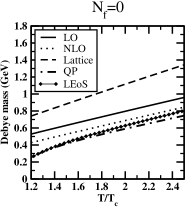
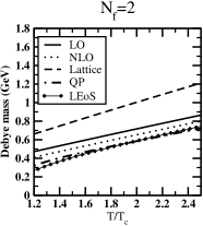
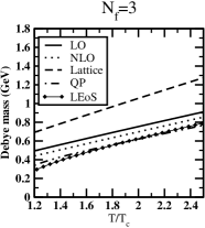
Figure 1: Debye mass verse temperature ($T/T_{c}$) for quasi particle (QP), lattice EoS, lattice parametrized, Next-to-leading order and leading order cases, when we used the fugacity equation of state EoS 1.Left panel represents the pure gluonic case, middle and right panel represents 2-flavour and 3-flavour respectively.

Here, we consider the quasi-particle description chandra1 ; chandra2 of $O(g^{5})$ hot QCD zhai ; arnold and $O(g^{6}\ln(1/g)$ hot QCD EoSs kajantie , we call them EoS1 and EoS2 respectively. We further consider the lattice QCD EoS  lattice_baz in terms of its quasi-particle description, we denote it as LEoS. Although there are more recent lattice results with improved lattice actions and more refined lattice lattice_hotqcd ; lattice_fodor , but to update the current model requires pure glue results for the trace anomaly with the same lattice set-up. Therefore, such attempts are beyond the scope of the present work. We intend to explore these possibilities in near future.

The equilibrium distribution function is written in the form given below:

$$f_{g,q}=\frac{z_{g,q}\exp(-\beta p)}{\bigg{(}1\mp z_{g,q}\exp(-\beta p)\bigg{)}}.$$ (6)

where $g$ stands for quasi-gluons, and $q$ stands for quasi-quarks. $z_{g}$ is the quasi-gluon effective fugacity and $z_{q}$ is quasi-quark effective fugacity. These distribution functions are isotropic in nature. These fugacities should not be confused with any conservation law (number conservation) and have merely been introduced to encode all the interaction effects at high temperature QCD. Both $z_{g}$ and $z_{q}$ have a very complicated temperature dependence and asymptotically reach to the ideal value unity chandra2 . The temperature dependence $z_{g}$ and $z_{q}$ fits well to the form given below,

$$z_{g,q}=a_{q,g}\exp\bigg{(}-\frac{b_{g,q}}{x^{2}}-\frac{c_{g,q}}{x^{4}}-\frac{d_{g,q}}{x^{6}}\bigg{)}.$$ (7)

(Here $x=T/T_{c}$ and $a$, $b$ and $c$ and $d$ are fitting parameters), for both EoS1 and EoS2.

The Debye mass, $m_{D}$ is defined in terms of the equilibrium (isotropic) distribution function as,

$$m_{D}^{2}\equiv-g^{2}\int\frac{{\rm d}^{3}\bar{\vec{p}}}{(2\pi)^{3}}\,\frac{{\rm d}f_{eq}(\bar{p})}{{\rm d}\bar{p}}.$$ (8)

where, $f_{eq}$ is taken to be a combination of ideal Bose-Einstein and Fermi-Dirac distribution functions as rebhan , and is given by:

$$f_{eq}=2N_{c}f_{g}(\vec{p})+2N_{f}(f_{q}(\vec{p})+f_{\bar{q}}(\vec{p})).$$ (9)

Since, we are dealing with the QGP system with vanishing baryon density, therefore, $f_{q}=f_{\bar{q}}$ (here, $f_{g}$ and $f_{q}$ are the quasi-parton thermal distributions given in Eq. (6)). This combination of $f_{eq}$ leads to the leading order HTL expression ($m_{D}^{2}=g^{2}(T)T^{2}(N_{c}/3+N_{f}/6)$) for the Debye mass in hot QCD. Here, $N_{c}$ denotes the number of colors and $N_{f}$ the number of flavors.

Now, considering quasi-parton distributions, we obtain, $m_{D}$ in the pure gluonic case:

$$m^{2}_{D}=g^{2}(T)T^{2}\bigg{(}\frac{N_{c}}{3}\times\frac{6PolyLog[2,z_{g}]}{\pi^{2}}\bigg{)}$$ (10)

and full QCD:

$$m^{2}_{D} = g^{2}(T)T^{2}\bigg{[}\bigg{(}\frac{N_{c}}{3}\times\frac{6PolyLog[2,z_{g}]}{\pi^{2}}\bigg{)}$$ (11)

$$+{\bigg{(}\frac{N_{f}}{6}\times\frac{-12PolyLog[2,-z_{q}]}{\pi^{2}}\bigg{)}}\bigg{]}.$$

Here, $g(T)$ is the QCD running coupling constant, $N_{c}=3$ ($SU(3)$) and $N_{f}$ is the number of flavor, the function $PolyLog[2,z]$ having form, $PolyLog[2,z]=\sum_{k=1}^{\infty}\frac{z^{k}}{k^{2}}$. We get same expressions from the chromo-electric response functions in chandra3 for the interacting QGP.

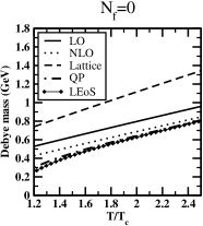
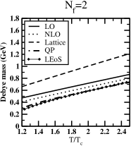
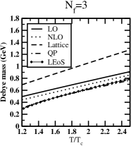
Figure 2: Debye mass verse temperature ($T/T_{c}$) for quasi particle (QP), lattice EoS, lattice parametrized , and leading order (LO) cases, when we used the fugacity equation of state EoS 2.Left panel represents the pure gluonic case, middle and right panel represents 2-flavour and 3-flavour respectively.

The medium modified $m_{D}$ in terms of effective fugacities can be understood by relating it with the charge renormalization in the medium. This could be done by defining the effective charges for the quasi-gluons and quarks as $Q_{g}$ and $Q_{q}$. These effective charges are given by the equations:

$$Q^{2}_{g} = g^{2}(T)\frac{6PolyLog[2,z_{g}]}{\pi^{2}}$$

$$Q^{2}_{q} = g^{2}(T)\frac{-12PolyLog[2,-z_{q}]}{\pi^{2}}.$$ (12)

Now the expressions for the Debye mass can be rewritten as,

$$m^{2}_{D}=\left\{\begin{array}[]{rcl}Q^{2}_{g}T^{2}\frac{N_{c}}{3}&\mbox{for pure gauge,}&\\ T^{2}(\frac{N_{c}}{3}Q^{2}_{g})+(\frac{N_{f}}{6}Q^{2}_{q})&\mbox{for full QCD}&\end{array}\right.$$ (13)

Here, $\{Q^{2}_{g},Q^{2}_{q}\}\leq g^{2}(T)$ since it acquire the ideal value $g^{2}(T)$ asymptotically. As mentioned earlier, the effective fugacities, $z_{g}$ and $z_{q}$ are obtained for EoS1, EoS 2 and LEoS. The Debye mass with LEoS using our quasi-particle model model is seen closer to that for EoS1 and EoS as compared to other cases. It is farthest as compared lattice Debye mass as the factor of $1.4$ in the definition of of the lattice Debye mass can not be reproduced by perturbative/improved perturbative QCD or transport theory.

The temperature dependence of the quasi-particle Debye mass, $m_{D}^{QP}$ in pure and full QCD with $N_{f}=2,3$ is depicted in Fig. 1 and Fig. 2, comparing it with the LO and NLO in HTL, and lattice parameterized Debye masses which are denoted as $m_{D}^{LO}$ , and $m_{D}^{L}$ respectively. These various Debye masses have the following mathematical expressions,

$$m_{D}^{LO} = g(T)T\sqrt{\frac{N_{c}}{3}+\frac{N_{f}}{6}},$$

$$m_{D}^{NLO} = m_{D}^{LO}+\frac{N_{c}g^{2}(T)T}{4\pi}\ln(\frac{m_{D}^{LO}}{g^{2}(T)T}),$$

$$m_{D}^{L} = 1.4g(T)T,$$

$$m_{D}^{QP} = g(T)T\bigg{[}\frac{2N_{c}}{3\pi^{2}}PolyLog[2,z_{g}]$$ (14)

$$-\frac{2N_{f}}{\pi^{2}}PolyLog[2,-z_{q}]\bigg{]}^{\frac{1}{2}}.$$

For $g(T)$, we employ two expression for the running coupling in finite temperature QCD laine_coupling . Clearly, $m_{D}^{QP}$ is lowest among all other cases for the whole range of temperature considered here. The $m_{D}^{LO}$ is higher and $m_{D}^{NLO}$, and $m_{D}^{L}$ is largest among them for the whole range of temperature. From its temperature dependence in Eq. (II.1), it is straightforward to see that it will approach to the $m_{D}^{LO}$ asymptotically ($z_{g,q}\rightarrow 1$). These observations are holding true for all ($N_{f}=0,2,3$) cases and for the EoS1 and ESO2.

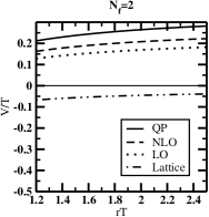
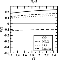
Figure 3: The behaviour of $V(r,T)/T$ as a function of $rT$ for a fixed ($T/T_{c}=3.32$) for EoS1. The left panel represents the pure gluonic, middle and right panel represents 2-flavour and 3-flavour respectively.

II.2 Heavy quark potential and quankonia Binding energies with EQPM

II.2.1 The Heavy-quark Potential

The heavy-quark potential given in Eq. (4) is shown as a function of $rT$ for fixed $T/T_{c}$ for pure gluonic, $N_{f}=2$ and $N_{f}=3$ cases in Fig. 3 (for EoS1) and Fig. 4 (EoS2) The expressions for the $m_{D}$ has been taken from Eq. (II.1) and employed in the expression for the potential in Eq. (4). As expected the potential as a function of $rT$ is lowest with the $m_{D}^{L}$ and highest for the $m_{D}^{QP}$ for the fixed $T$ for the entire range of $rT$ (this just follows from the temperature dependence of the Debye mass i. e., higher the Debye mass higher the screening). The similar observations are seen for $N_{f}=2$ and $3$ and for both EoS1 and EoS2.

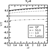
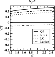
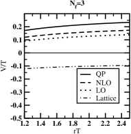
Figure 4: The behaviour of $V(r,T)/T$ as a function of $rT$ for a fixed ($T/T_{c}=3.32$) for EoS2. The left panel represents the pure gluonic, middle and right panel represents 2-flavour and 3-flavour respectively.

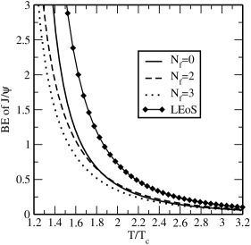
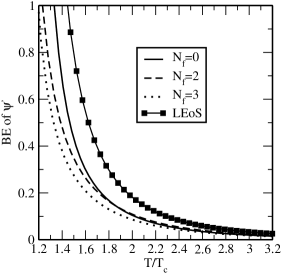
Figure 5: Dependence of binding energy(in $GeV$) of (a) $J/\psi$ and (b) $\psi^{\prime}$ on temperature $T/T_{c}$ with fugacity equation of state EoS1

.

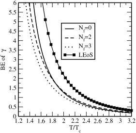
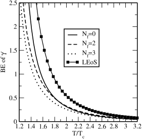
Figure 6: Dependence of binding energy(in $GeV$) of (a) $\Upsilon$ and (b) $\Upsilon^{\prime}$ on temperature $T/T_{c}$ with fugacity equation of state EoS1

.

II.2.2 The Binding Energies of $J/\Psi$ and $\Upsilon$

To obtain the binding energy (BE) with heavy quark potential in Eq. (4), we need to solve the Schrödinger equation numerically with the full medium dependent complex potential kaka . Clearly, the binding energy will have both real and the imaginary parts. One can take the intersection point of real and imaginary parts of the binding energies while plotting their temperature dependences to define the dissociation temperature of quarkonia state under consideration. Another approach to look at the quarkonia dissociation is to first compute the thermal width of the given quarkonia from the imaginary part of the potential and equate it with the twice of the binding energies (real part). We follow the latter approach to estimate the dissociation temperatures. Therefore, we shall mostly concentrate on the the real part of the binding energies and thermal width of the quarkonia.

In the limiting case discussed earlier, the real part of the medium modified potential resembles to the hydrogen atom problem matsui . The solution of the Schrödinger equation gives the eigenvalues for the ground states and the first excited states in charmonium ($J/\psi$, $\psi^{\prime}$ etc.) and bottomonium ($\Upsilon$, $\Upsilon^{\prime}$ etc.) spectra :

$$E_{n}=-\frac{1}{n^{2}}\frac{m_{Q}\sigma^{2}}{m^{4}_{D}},$$ (15)

where $m_{Q}$ is the mass of the heavy quark.

In the present case, we solve the Schrödinger equation with full potential and obtain the binding energies. The temperature dependence of the binding energies are shown in Figs. 5-8. For our analysis here, we consider $J/\Psi$, $\Psi^{\prime}$ binding energies with EoS 1 and EoS 2 as a function of temperature in Fig. 5 and Fig. 7 respectively. On the other hand for $\Upsilon$ and $\Upsilon^{\prime}$ with these equations of state in Fig. 6 and Fig. 8.

We have also plotted the LEoS estimates for BEs of various quarkonia states based on its quasi-particle understanding along with prediction for EoS1 and EoS2. The BE in this case is largest as compared to $N_{f}=0,2,3$ using EoS1 and EoS2 for the considered range of temperature.This observations is seen to be valid for not only $J/\psi$, $\Psi^{\prime}$ but also$\Upsilon$ and $\Upsilon^{\prime}$ states. In each of the cases, the behavior is shown for $N_{f}=0,2$ and $3$. There are some interesting observations that could be made while having a closer look at the temperature dependence of the binding energies in each case. Comparing the $J/\Psi$ and $\Psi^{\prime}$ cases, we see that the binding energy is approaching to zero sharply in the later case. This roughly implies that the latter state will dissolve before the former one. The same statement could me made for $\Upsilon$ and $\Upsilon^{\prime}$ states i. e., the former will dissociate later in temperature as compared to the latter state. We shall see that these observations are indeed true while we estimate the dissociation temperature for these states later. Interesting, for the three cases ($N_{f}=0,2,3$) with either EoS 1 and EoS 2 , these predictions for the dissociation temperatures come out true.

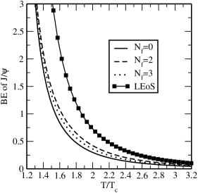
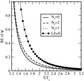
Figure 7: Dependence of binding energy(in $GeV$) of (a) $J/\psi$ and (b) $\psi^{\prime}$ on temperature $T/T_{c}$ with fugacity equation of state EoS2

.

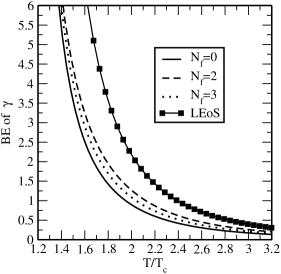
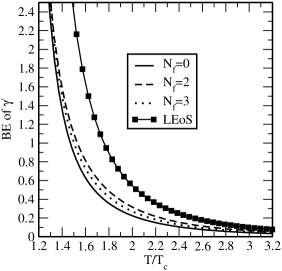
Figure 8: Dependence of binding energy(in $GeV$) of (a) $\Upsilon$ and (b) $\Upsilon^{\prime}$ on temperature $T/T_{c}$ with fugacity equation of state EoS2

.

Let us now proceed to the computation of the dissociation temperatures for the above mentioned quarkonia bound states. To that end, we need to compute the imaginary part of the heavy-quark potential and thus estimate the thermal width.

III The complex inter-quark potential

Here, we discuss how to obtain the the complex inter-quark potential. The real part of the potential will be same as Eq. (4). We follow the similar procedure to obtain the imaginary part of the potential as discussed below. To obtain the imaginary part of the inter-quark potential, we first need to obtain the imaginary part of the symmetric self energy in the static limit. This can be done by obtaining the imaginary part of the HTL propagator which represents the inelastic scattering of an off-shell gluon to a thermal gluon nora1 ; const2 ; Laine:2007qy ; Escobedo:2008sy . The imaginary part of the potential plays crucial role in weakening the bound state peak or transforming it to mere threshold enhancement and eventually in dissociating it (finite width ($\Gamma$) for the resonance peak in the spectral function, is estimated from the imaginary part of the potential which, in turn, determines the dissociation temperatures for the respective quarkonia). This sets the dissociation criterion, i. e., it is expected to occur while the (twice) binding energy becomes equals the width $\sim\Gamma$ mocsy ; Burnier:2007qm . The equality will do the quantitative determination of the dissociation temperature.

To obtain the imaginary part of the potential in the QGP medium, the temporal component of the symmetric propagator in the static limit has been considered as laine ,

$$ImD^{00}_{F(iso)}(0,k)=\frac{-2\pi Tm_{D}^{2}}{k(k^{2}+m_{D}^{2})^{2}}.$$ (16)

The same expression Eq. (16) could also be obtained for partons with space-like momenta ($\omega^{2}<k^{2}$) from the retarded (advanced) self energy Dumitru:2009fy using the relation const2 ; laine :

$$\ln\frac{\omega+k\pm i\epsilon}{\omega-k\pm i\epsilon}=\ln|\frac{\omega+k}{\omega-k}|\mp i\pi\theta(k^{2}-{\omega}^{2})~{}.$$ (17)

The imaginary part of the symmetric propagator Eq. (16) leasds to the the imaginary part of the dielectric function in the QGP medium as:

$$\frac{1}{\epsilon(k)}=-\pi Tm_{D}^{2}\frac{k^{2}}{k(k^{2}+m_{D}^{2})^{2}}.$$ (18)

Afterwards, the imaginary part of the in medium potential is easy to obtain owing the definition of the potential Eq. (1) as mentioned in utt :

$$ImV(r,T) = -\int\frac{d^{3}\mathbf{k}}{(2\pi)^{3/2}}(e^{i\mathbf{k}\cdot\mathbf{r}}-1)$$ (19)

$$\times\left(-\sqrt{\frac{2}{\pi}}\frac{\alpha}{k^{2}}-\frac{4\sigma}{\sqrt{2\pi k^{4}}}\right)\frac{-\pi Tm_{D}^{2}\ k}{(k^{2}+m_{D}^{2})^{2}}$$

$$\equiv ImV_{1}(r,T)+ImV_{2}(r,T)~{},$$

where $ImV_{1}(r,T)$ and $ImV_{2}(r,T)$ are the imaginary parts of the potential due to the medium modification to the short-distance and long-distance terms, respectively:

$$ImV_{1}(r,T) = -\frac{\alpha}{2\pi^{2}}\int d^{3}\mathbf{k}(e^{i\mathbf{k}\cdot\mathbf{r}}-1)$$ (20)

$$\times\left[\frac{\pi Tm_{D}^{2}}{k(k^{2}+m_{D}^{2})^{2}}\right],$$

$$ImV_{2}(r,T) = -\frac{4\sigma}{({2\pi})^{2}}\int\frac{d^{3}{\bf k}}{(2\pi)^{3/2}}(e^{i{\bf k}\cdot{\bf r}}-1)$$ (21)

$$\times\frac{1}{k^{2}}\left[\frac{\pi Tm_{D}^{2}}{k(k^{2}+m_{D}^{2})^{2}}\right].$$

After performing the integration, the contribution due to the short-distance term to imaginary part becomes (with $z=k/m_{D}$)

$$ImV_{1}({\bf r},T) = 2\alpha T\int_{0}^{\infty}\frac{zdz}{(z^{2}+1)^{2}}\left(1-\frac{\sin{z\hat{r}}}{z\hat{r}}\right)$$ (22)

$$\equiv \alpha T\phi_{0}(\hat{r}),$$

and the contribution with the non-zero string tension becomes:

$$ImV_{2}(r,T) = \frac{4\sigma T}{m_{D}^{2}}\int_{0}^{\infty}\frac{dz}{z(z^{2}+1)^{2}}\left(1-\frac{\sin{z\hat{r}}}{z\hat{r}}\right)$$ (23)

$$\equiv \frac{2\sigma T}{m_{D}^{2}}\psi_{0}(\hat{r})~{},$$

where the functions, $\phi_{0}(\hat{r})$ and $\psi_{0}(\hat{r})$ at leading-order in $\hat{r}$ are

$$\phi_{0}(\hat{r}) = \left(-\frac{{\hat{r}}^{2}}{9}\left(-4+3\gamma_{E}+3\log\hat{r}\right)\right).$$ (24)

$$\psi_{0}(\hat{r}) = \frac{\hat{r}^{2}}{6}+\left(\frac{-107+60\gamma_{E}+60\log(\hat{r})}{3600}\right)\hat{r}^{4}+O(\hat{r}^{5}).$$

In the short-distance limit ($\hat{r}\ll 1$), both the contributions, at the leading logarithmic order, reduce to

$$ImV_{1}(r,T)=\alpha T\frac{{\hat{r}^{2}}}{3}\log(\frac{1}{\hat{r}}),$$ (26)

$$ImV_{2}(r,T)=-\frac{2\sigma T}{m_{D}^{2}}\frac{{\hat{r}^{4}}}{60}\log(\frac{1}{\hat{r}}).$$ (27)

Therefore, the sum of Coulomb and string tension dependent terms leads to the the imaginary part of the potential:

$$ImV(r,T)=T\left(\frac{\alpha{\hat{r}^{2}}}{3}-\frac{\sigma{\hat{r}}^{4}}{30m_{D}^{2}}\right)\log(\frac{1}{\hat{r}}).`$$ (28)

One thus immediately observes that for small distances the imaginary part vanishes and its magnitude is smaller as compared to the case with only the Coulombic term Dumitru:2009fy . The effect of non-perturbative contribution coming from the string terms, thus, reduces the width of the resonances in thermal medium. The imaginary part of the potential above, provides an estimate for the width ($\Gamma$) for a resonance state. The width $\Gamma$ can be computed in first-order perturbation, while folding the imaginary part of the potential with the unperturbed (1S) Coulomb wave function as:

$$\Gamma=\left(1+\frac{3\sigma}{\alpha m_{Q}^{2}}\right)~{}\frac{4T}{\alpha}{\frac{m_{D}^{2}}{m_{Q}^{2}}}~{}\log\frac{\alpha m_{Q}}{2m_{D}}.$$ (29)

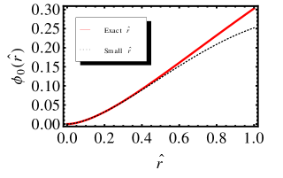
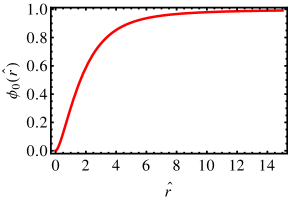
Figure 9: Dependence of $\phi_{0}(\hat{r})$ on $\hat{r}$. The lower panel shows the comparison between the small $\hat{r}$ approximation and exact one.

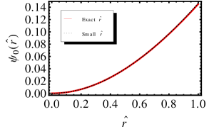
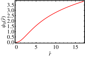
Figure 10: Dependence of $\psi_{0}(\hat{r})$ on $\hat{r}$. The figure in the left shows the comparison between the small $\hat{r}$ approximation and exact results. The right figure depicts the exact results until $\hat{r}=17$ beyond which fluctuations start showing up and grow rapidly.

It is possible to solve the integral for the functions $\phi_{0}(\hat{r})$ and $\psi_{0}(\hat{r})$ in the right hand side of the Eq. (23) exactly. The compact mathematical expressions are presented in the Appendix. The behavior of these functions as a function of $\hat{r}$ is depicted in Figs. 9 and 10 where we have compared the small $\hat{r}$ behavior in Eq. (27) with approximate result in Eqs. (24) and (III) along with results for larger $\hat{r}$. Clearly the approximation works fantastically well of $\hat{r}<1$ for $\phi_{0}(\hat{r})$ and better for $\psi_{0}(\hat{r})$. The behavior at large $\hat{r}$ is crucial to understand the fate of higher (excited) states of quarkonia. The analytic estimate for $\psi_{0}(\hat{r})$ based on the expression quoted in the appendix is well behaved until $\hat{r}\leq 16-17$. For $\hat{r}>17$ the functions $\psi_{0}(\hat{r})$ show large fluctuations that grow rapidly for larger $\hat{r}$. Therefore, in that region, we perhaps can not utilize it for phenomenological purposes.

III.1 The dissociation temperatures for heavy quarkonia

There are two criteria for the dissociation of quarkonia bound state in the QGP medium that are under consideration here. The first one is the dissociation of a given quarkonia bound state by the thermal effects alone. On the other hand, the second criterion is based on the dissolution of a given quarkonia state while its thermal width is overcomed by the twice of the real part of the binding energy. We shall employ both of them one by one below and present the comparison of the quantitative estimates of the dissociation temperatures.

III.1.1 Dissociation by thermal effects

Dissociation of a quarkonia bound state in a thermal QGP medium will occur whenever the binding energy (BE), $E_{B}$ of the said state will fall below the mean thermal energy of a quasi-parton. In such situations the thermal effect can dissociate the quakonia bound state.

Table 1: Lower(upper) bound on the dissociation temperature($T_{D}$) for the quarkonia states (in units of $T_{c}$)for using fugacity parameters of EoS 1

. State Pure QCD $N_{f}=2$ $N_{f}=3$ $J/\psi$ 1.6(1.9) 1.6(2.1) 1.5(2.0) $\psi^{\prime}$ 1.3(1.5) 1.3(1.6) 1.3(1.5) $\Upsilon$ 1.9(2.4) 2.1(2.6) 2.0(2.5) $\Upsilon^{\prime}$ 1.5(1.8) 1.6(1.9) 1.5(1.9)

To obtain the lower bound of the dissociation temperatures of the various quarkonia states, the (relativistic) thermal energy of the partons will be $3\ T$. On the other hand, the upper bound of the dissociation temperature ($T_{D}$) is obtained by considering the mean thermal energy to be $T$. The dissociation is supposed to occur whenever,

$$E_{B}(T_{D})=3T_{D}\ \textbf{or}\ T_{D}.$$ (30)

While solving for the $E_{B}$, the string tension ($\sigma$) is taken as $0.184$ ${\rm{GeV}^{2}}$, and critical temperatures ($T_{c}$) are considered as $270MeV$, $203MeV$ and $197MeV$ for pure, 2-flavor and 3-flavor QCD at high temperature for both the equations of state. The binding energies are shown as a function of temperature in earlier plots. The dissociation temperatures for the ground state and the first excited state of $c\bar{c}$ ($J/\Psi$ and $\Psi^{\prime}$) and $b\bar{b}$ sates ($\Upsilon$ and $\Upsilon^{\prime}$) are presented in Table I and III while considering two different criteria of quarkonia dissociation.

Table 2: Lower(upper) bound on the dissociation temperature($T_{D}$) for the quarkonia states (in units of $T_{c}$)for using fugacity parameters of EoS 2

. State Pure QCD $N_{f}=2$ $N_{f}=3$ $J/\psi$ 1.5(1.8) 1.7(2.0) 1.6(1.9) $\psi^{\prime}$ 1.2(1.4) 1.3(1.6) 1.3(1.6) $\Upsilon$ 1.8(2.2) 2.0(2.6) 2.0(2.5) $\Upsilon^{\prime}$ 1.4(1.7) 1.6(1.9) 1.6(1.9)

III.1.2 Overcoming thermal width of the resonance by the binding energy

Whenever the thermal width, $\Gamma$ of the a given quarkonium is as large as twice the binding energy (real part) the given quarkonia state will dissolve utt

Table 3: The dissociation temperature($T_{D}$) for the quarkonia states (in units of $T_{c}$)for using fugacity parameters of EoS 1, when thermal width =2 BE

. State Pure QCD $N_{f}=2$ $N_{f}=3$ $J/\psi$ 1.8 2.0 1.9 $\psi^{\prime}$ 1.6 1.8 1.8 $\Upsilon$ 2.6 2.8 2.2 $\Upsilon^{\prime}$ 2.1 2.2 2.1

Table 4: The dissociation temperature($T_{D}$) for the quarkonia states (in units of $T_{c}$)for using fugacity parameters of EoS 2, when thermal width =2 BE

. State Pure QCD $N_{f}=2$ $N_{f}=3$ $J/\psi$ 1.7 1.9 1.9 $\psi^{\prime}$ 1.5 1.7 1.7 $\Upsilon$ 2.5 2.7 2.6 $\Upsilon^{\prime}$ 2.0 2.2 2.1

We applied the criteria for the $c\bar{c}$ bound states ($J/\psi$ and $\psi^{\prime}$) and $b\bar{b}$ bound state ($\Upsilon$ and $\Upsilon^{\prime}$). The quantitative estimates for the respective dissociation temperatures are enlisted in Tables II and IV.

Table 5: Lower(upper) bound on the dissociation temperature($T_{D}$) for the quarkonia states for 2+1 flavour (in units of $T_{c}$) case while using the fugacity parameters of the LEoS (second row). The third row records the estimates with second criterion of the dissociation ( 2  BE $\equiv$ thermal width)

State	$J/\psi$	$\psi^{\prime}$	$\Upsilon$	$\Upsilon^{\prime}$
LEoS	1.9(2.3)	1.5(1.8)	2.3(2.8)	1.8( 2.1)
LEoS	2.1	1.8	3.1	2.6

Let us now analyze the quantitative estimates for $J/\psi$ and $\psi^{\prime}$ dissociation temperatures for EoS1 equating the thermal width with the twice of the BE. The $J/\psi$ state is seen to dissociate at $T=1.8T_{c}$ for $N_{f}=0$ , $T=2.0T_{c}$ for $N_{f}=2$ and for $N_{f}=3$ at $T=1.9T_{c}$. On the $\Psi^{\prime}$ is seen to dissociate at $T=1.6T_{c}$ for $N_{f}=0$ , $T=1.8T_{c}$ for $N_{f}=2$ and for $N_{f}=3$ at $T=1.8T_{c}$. On the other hand, for EoS2, $J/\psi$ is seen to dissociate at $T=1.7T_{c}$ for $N_{f}=0$ , $T=1.9T_{c}$ for $N_{f}=2$ and for $N_{f}=3$ at $T=1.9T_{c}$. $\Psi^{\prime}$ is seen to dissociate at $T=1.5T_{c}$ for $N_{f}=0$ , $T=1.7T_{c}$ for $N_{f}=2$ and for $N_{f}=3$ at $T=1.7T_{c}$ . As stated earlier (on the basis of temperature dependence of the BE ) $\Psi^{\prime}$ is seen to dissociate at lower temperatures as compared to $J/\psi$ for both the equations of state.

Similarly, for $\Upsilon$ and $\Upsilon^{\prime}$ dissociation temperatures are recorded in Table III and Table IV. The $\Upsilon$ state is seen to dissociate at $T=2.6T_{c}$ for $N_{f}=0$ , $T=2.8T_{c}$ for $N_{f}=2$ and for $N_{f}=3$ at $T=2.2T_{c}$ while employing EoS1 through the quasi-particle picture. On the other hand, $\Upsilon^{\prime}$ is seen to dissociate at $T=2.1T_{c}$ for $N_{f}=0$ , $T=2.2T_{c}$ for $N_{f}=2$ and for $N_{f}=3$ at $T=2.1T_{c}$ for the same EoS. With EoS2, $\Upsilon$ is seen to dissociate at $T=2.5T_{c}$ for $N_{f}=0$ , $T=2.7T_{c}$ for $N_{f}=2$ and for $N_{f}=3$ at $T=2.6T_{c}$ and $\Upsilon^{\prime}$ is seen to dissociate at $T=2.0T_{c}$ for $N_{f}=0$ , $T=2.2T_{c}$ for $N_{f}=2$ and for $N_{f}=3$ at $T=2.1T_{c}$. Again, we can see (on the basis of temperature dependence of the BE ) that $\Upsilon$ is seen to dissociate at higher temperatures as compared to $\Upsilon^{\prime}$ for both the equations of state.

The estimates for various quarkonia states under consideration with LEoS are quoted in Table V. The first row records the estimates for the case while the quarkonia dissociation has been led by the average thermal energy of the $q/\bar{q}$. On the other hand the second row captures estimates while the BEs are overcomed by the thermal width of quarkonia due to complex nature of the potential(inter-quark). The upper bound obtained in row1 are closer to those with the latter criterion. On comparing the estimate only slightly different.

Comparing the numbers for the $T_{D}$ for various quarkonia states, quoted in Table I and Table III , we observe that the quantitative estimates in Table III are quite closer to the upper bound(NR) criteria. Note that the former estimates are based on the dissolution of a given quarkonia state by the mean thermal energy of the quasi-partons in the hot QCD/QGP medium, the latter one is based on equating the thermal width to the real part of the binding energy (twice). Similar observations are obtained while comparing the estimates from Table II and Table IV. Interesting, the numbers obtained by employing EoS1 and EoS2 with the latter criterion of quarkonia dissociation, the estimates are not very different from each other.

IV Results and Discussion

The Hot QCD equations of state corresponding to interactions up to $O(g^{5})$ and $O(g^{6}(ln1/g))$ in the improved perturbative QCD can significantly impact the fate of quarkonia in the QGP medium. The medium modified form of the heavy quark-potential in which the medium modification causes the Debye screening of color charges, have been obtained by employing the Debye mass obtained by utilizing the quasi-particle understanding of these equations of state. This, in turn, leads to the temperature dependent binding energies for the $J/\psi$ and $\psi^{\prime}$. The binding energies are seen to decreases less sharply for pure gluonic case in comparison to full QCD medium. Similar pattern have been observed for the case of $\Upsilon$ and $\Upsilon^{\prime}$ states.

To estimate the dissociation temperature, we consider two criteria viz. the dissociation by mean thermal energy of the quasi-particles in the QGP medium and, the binding energy overcoming the thermal width of the quakonia bound state. The upper and lower bound within the first criterion were obtained by thermal energy $T$ and $3T$, respectively. In numbers for the dissociation temperatures from both the criteria are seen to be consistent with the recent predictions from the recent quarkonium spectral function studies using a potential model. The effects of realistic EoS for the QGP have significant impact on the binding energies and the dissociation temperatures for the various quarkonia states.

V Conclusion and outlook

In conclusion, we have studied the quarkonia dissociation in QGP in the isotropic case employing quasi-parton equilibrium distribution functions obtained from $O(g^{5})$ and $O(g^{6}(ln1/g))$ hot QCD equations of state and LEoS and medium modification to a heavy quark potential. We have found that medium modification causes a dynamical screening of color charge which, in turn, leads to a temperature dependent of binding energy. We have systematically studied the temperature dependence of binding energy for the ground and first excited states of charmonium and bottomonium spectra in pure gluonic and full QCD medium. We have then determined the dissociation of heavy Quarkonium in hot QCD medium by employing the medium modification to a heavy quark potential and explore how the pattern changes for pure gluonic case and full QCD in the Debye mass.

We intend to look for extensions of the present work in the case of hydrodynamically expanding viscous QGP medium. Another, interesting direction would be to couple the analysis to the physics of momentum anisotropy and instabilities in the early stages of the heavy-ion collisions and its impact on the physics of heavy quarkonia dissociation and yields in heavy-ion collisions.

Appendix A Imaginary part of inter-quark potential

It is possible to solve the integral in , Eq.(22) and Eq.(23) for real $\hat{r}$. The expression for the function $\phi^{0}(\hat{r})$ and $\psi^{0}(\hat{r})$ are obtained as:

$$\phi_{0}(\hat{r}) = 1-\sqrt{\pi}G_{1,3}^{2,1}\left(\frac{\hat{r}^{2}}{4}\ {}\Bigg{|}\ {}{{0}\atop{0},{1},{-\frac{1}{2}}}\right),$$

$$\psi_{0}(\hat{r}) = \frac{1}{2|\hat{r}|}\Bigg{(}-6|\hat{r}|+4|\hat{r}|\gamma_{E}+4\hat{r}Log[|\hat{r}|]$$

$$+\Big{(}Ci\big{(}-i|\hat{r}|\big{)}+Ci\big{(}i|\hat{r}|\big{)}\Big{)}$$

$$\times\bigg{[}|\hat{r}|\cosh\big{(}|\hat{r}|)-3\sinh\big{(}|\hat{r}|\big{)}\bigg{]}$$

$$+2Shi\big{(}|\hat{r}|\big{)}\bigg{[}3\cosh\big{(}|\hat{r}|)-\hat{r}|\sinh\big{(}|\hat{r}|\big{)}\bigg{]}\Bigg{)}.$$

Here, $G$ is MeijerG function and

$$Ci(z) = CosIntegral(z)=-\int_{z}^{\infty}\frac{\cos(t)}{t}dt,$$

$$Shi(z) = SinhIntegral(z)=\int_{0}^{z}\frac{\sinh(t)}{t}dt$$

References

- (1) M. J. Leitch [PHENIX Collaboration], arXiv: 0806.1244 [nucl-ex].
- (2) T. Matsui, and H. Satz, Phys. Lett. B 178, 416 (1986).
- (3) M. Laine, Nucl. Phys. A 820, 25C (2009).
- (4) D Pal, Binoy Krishna Patra and D K Srivastava, Eur. Phys.J.C 17, 179 (2000).
- (5) Binoy Krishna Patra and D K Srivastava, Phys. Lett. B 505, 113 (2001).
- (6) Binoy Krishna Patra, V. J. Menon, Nucl. Phys. A 708, 353 (2002).
- (7) Binoy Krishna Patra and V. J. Menon, Eur. Phys. J. C 37, 115 (2004).
- (8) Y. Burnier, M. Laine, M. Vepsáláinen, Phys. Lett. B 678, 86 (2009).
- (9) W. Lucha, F. F. Schoberl and D. Gromes, Phys. Rept. 200, 127 (1991).
- (10) E. Eichten, K. Gottfried, T. Kinoshita, J. B. Kogut, K. D. Lane and T. M. Yan, Phys. Rev. Lett. 34, 369 (1975).
- (11) H. Iida, T. Doi, N. Ishii, H. Suganuma, and K. Tsumura, Phys. Rev. D 74, 074502 (2006).
- (12) A. Jakovac, P. Petreczky, K. Petrov, and A. Velytsky, Phys. Rev. D 75, 014506 (2007).
- (13) Agnes Mocsy, Eur.Phys. J C, 61, 705 (2009).
- (14) E. V. Shuryak and I. Zahed, Phys. Rev. D 70, 054507 (2004).
- (15) C. Y. Wong, Phys. Rev. C 72, 034906 (2005).
- (16) D. Cabrera and R. Rapp, Phys. Rev. D 76, 114506 (2007).
- (17) H. Satz, Nucl. Phys. A 783, 249 (2007).
- (18) L. Thakur, N. Haque, U. Kakade, and Binoy Krishna Patra, Phys. Rev. D 88, 054022 (2013).
- (19) T. Umeda, Phys. Rev. D 75, 094502 (2007).
- (20) W. M. Alberico, A. Beraudo, A. De Pace, and A. Molinari, Phys. Rev. D 77, 017502 (2008).
- (21) A. Pineda and J.Soto, Nucl.Phys. Proc. Suppl. 64, 428 (1998); N.Brambilla, A.pineda, J.soto and A.Vairo, Rev.Mod.Phys.77, 1423 (2005).
- (22) L. Thakur, U. Kakade, and Binoy Krishna Patra, Phys. Rev. D 89, 094020 (2014).
- (23) P. K. Srivastava, Lata Thakur, B.K. Patra, Phys. Rev. C 91, 044903 (2015).
- (24) M. A. Escobedo, F. Giannuzzi, M. Mannarelli and J. Soto, Phys. Rev. D 87, 114005 (2013).
- (25) E. V. Shuryak, Phys. Rept. 61, 71 (1980); D. J. Gross, R. D. Pisarki and L.G. Yaffe, Rev. Mod. Phys. 53, (1981).
- (26) M. Laine, J. High. Energy Phys. 04, 124 (2011).
- (27) M. He, R. J. Fries, R. Rapp, Phys. Lett. B 701, 445 (2011).
- (28) Nora Brabilla, Antonio Pineda, Joan Soto, Antonio Vairo, Rev. Mod. Phys., 77, 1423 (2005).
- (29) Agnes Mocsy, P. Petreczky, Euro. Phys. J C 43, 77 (2005); Phys. Rev.D 73, 074007 (2006); Phys. Rev. Lett. 99, 211602 (2007).
- (30) T. Umeda, Phys. Rev. D 75, 017502 (2007).
- (31) V. Agotiya, Vinod Chandra, B. K. Patra, Phys. Rev.C 80, 025210 (2009).
- (32) B. K. Patra, V. Agotiya, Vinod Chandra, Eur. Phys. J. C 67, 465 (2010).
- (33) Saumen Datta, Frithjof Karsch, Peter Petreczky, Ines Wetzorke, Phys. Rev.D 69, 094507 (2004).
- (34) Nora Brambilla, Jacopo Ghiglieri, Peter Petreczky, Antonio Vairo, Phys. Rev. D 78, 014017 (2008).
- (35) M. Asakawa, T. Hatsuda, and Y. Nakahara, Nucl. Phys. A 715, 863 (2003); M. Asakawa and T. Hatsuda, Phys. Rev. Lett. 92 012001 (2004).
- (36) A. Jakovac, P. Petreczky, K. Petrov, and A. Velytsky, Phys. Rev. D 75, 014506 (2007).
- (37) T. Umeda, K. Nomura, and H. Matsufuru, Eur. Phys. J.C 39, 9 (2005).
- (38) H. Iida et. al Phys. Rev. D 74, 074502 (2006).
- (39) W. M. Alberico, A. Beraudo, A. De Pace, A. Molinari, Phys.Rev.D 72, 114011 (2005); Phys. Rev. D 77, 017502 (2008).
- (40) C. Y. Wong and H. W. Crater, Phys. Rev. D 75 034505 (2007).
- (41) D. Cabrera and R. Rapp, Phys. Rev. D 76, 114506 (2007).
- (42) A. Mocsy and P. Petreczky, Phys. Rev. D 77, 014501 (2008).
- (43) Nora Brambilla, Antonio Pineda, Joan Soto, Antonio Vairo Rev.Mod.Phys.77, 1423 (2005).
- (44) A. Dumitru, Y. Guo and M. Strickland, arxiv: 0903.4703.
- (45) M. Laine, O. Philipsen, P. Romatschke, M. Tassler, JHEP 0703, 054 (2007).
- (46) V. Chandra, A. Ranjan, V. Ravishankar, Eur. Phys. J A 40, 109 (2009).
- (47) Vinod Chandra, R. Kumar, V. Ravishankar, Phys. Rev. C 76, 054909 (2007).
- (48) Vinod Chandra, A. Ranjan, V. Ravishankar, Euro. Phys. J C 40, 109 (2009).
- (49) Vinod Chandra, V. Ravishankar Phys. Rev. D 84, 074013 (2011).
- (50) N. Brambilla, et al., Rev. Mod. Phys. 77, 1423 (2005).
- (51) L. Kluberg, H. Satz, arXiv:hep-ph/0901.3831.
- (52) P. Petreczky, Eur. Phys. J. C 43 (2005) 51.
- (53) A. Rothkopf, T. Hatsuda and S. Sasaki, Phys. Rev. Lett. 108 (2012) 162001
- (54) R. A Schneider, Phys. Rev. D 66, 036003 (2002).
- (55) V. Agotiya, L. Devi, U. Kakade and B. K. Patra, Int. J. Mod. Phys.A 1250009 (2012).
- (56) M. Laine, O. Philipsen, M. Tassler and P. Romatschke, JHEP 03,054 (2007).
- (57) A. Beraudo, J. P. Blaizot, C. Ratti, Nucl. Phys. A 806, 312 (2008).
- (58) H. Satz, J. Phys. G: Nucl. Part. Phys.32, R25 (2006).
- (59) Peter Arnold, Chengxing Zhai Phys.Rev. D 51, 1906 (1995).
- (60) E. Shuryak, Sov. Phys. JETP 47, 212 (1978).
- (61) Anton Rebhan, Phys. Rev. D 48, 3967 (1993).
- (62) Eric Braaten and Agustin Nieto, Phys. Rev. Lett. 73, 2402 (1994).
- (63) Y. Burnier, A. Rothkopf, Phys. Lett. B 753, 232-236 (2016).
- (64) K. Kajantie, M. Laine, J. Peisa, A. Rajantie, K. Rummukainen, M.E. Shaposhnikov, Phys. Rev. Lett. 79 3130, (1997) ; A. Hart, M. Laine, O. Philipsen, Nucl. Phys. B 586, 443 (2000); O. Philipsen, M. Laine, M. Vepsalainen, J. High Energy Phys. 0909, 023 (2009).
- (65) C.E. Detar, J.B. Kogut, Phys. Rev. Lett. 59, 399 (1987); M. Cheng, S. Datta, A. Francis, J. van der Heide, C. Jung, O. Kaczmarek, F. Karsch, E. Laermann, et al., Eur. Phys. J. C 71, 1564 (2011); A. Bazavov, F. Karsch, Y. Maezawa, S. Mukherjee, P. Petreczky, Phys. Rev. D 91 (5), 054503 (2015).
- (66) S. Nadkarni, Phys. Rev. D 33 (1986) 3738; S. Nadkarni, Phys. Rev. D 34 3904 (1986); Y. Maezawa, et al., WHOT-QCD Collaboration, Phys. Rev. D 75 074501 (2007); Y. Maezawa, T. Umeda, S. Aoki, S. Ejiri, T. Hatsuda, K. Kanaya, H. Ohno, Prog. Theor. Phys. 128 955 (2012); S. Digal, O. Kaczmarek, F. Karsch, H. Satz, Eur. Phys. J. C 43, 71 (2005).
- (67) V. Goloviznin and H. Satz, Z. Phys. C 57, 671 (1994).
- (68) A. Peshier, B. Kampfer, O. P. Pavlenko and G. Soff, Phys. Rev. D 54, 2399 (1996).
- (69) M. D’Elia, A. Di Giacomo, E. Meggiolaro, Phys. Lett. B 408, 315 (1997); Phys. Rev. D 67, 114504 (2003); P. Castorina, M. Mannarelli, Phys. Rev. C 75, 054901 (2007); Phys. Lett. B 664, 336 (2007).
- (70) A. Dumitru, R. D. Pisarski, Phys. Lett. B 525, 95 (2002); K. Fukushima, Phys. Lett. B 591, 277 (2004); S. K. Ghosh et. al, Phys. Rev. D 73, 114007 (2006); H. Abuki, K. Fukushima, Phys. Lett. B 676, 57 (2006); H. M. Tsai, B. Mu?ller, J. Phys. G 36, 075101 (2009).
- (71) P. K. Srivastava, S. K. Tiwari, and C. P. Singh, Phys. Rev. D 82, 014023 (2010).
- (72) Chengxing Zhai, Boris Kastening Phys. Rev. D 52, 7232 (1995).
- (73) K. Kajantie, M. Laine, K. Rummukainen, Y. Schroder Phys. Rev. D 67, 105008 (2003).
- (74) M. Cheng et al., Phys. Rev. D 77, 014511 (2008); A. Bazavov et al., Phys. Rev. D 80, 014504 (2009)
- (75) A. Bazavov et al., Phys. Rev. D 90, 094503 (2014).
- (76) [71] S. Borsanyi, Z. Fodor, C. Hoelbling, S. D. Katz, S. Krieg, and K. K. Szabo, Phys. Lett. B 370, 99 (2014).
- (77) M. E. Carrington, A. Rebhan, Phys. Rev. D 79, 025018 (2009).
- (78) Vinod Chandra, V. Ravishankar, Euro. Phys. J C 59, 705 (2009).
- (79) M. Laine and Y. Schröder, JHEP 03, 067 (2005).
- (80) M. Laine, O. Philipsen and M. Tassler, JHEP 0709 (2007) 066.
- (81) M. A. Escobedo and J. Soto, Phys. Rev. A 78 (2008) 032520.
- (82) Y. Burnier, M. Laine and M. Vepsalainen, JHEP 0801 (2008) 043.
- (83) A. Dumitru, Y. Guo and M. Strickland, Phys. Rev. D 79 (2009) 114003.
- (84) Lata Thakur, Uttam Kakade and Binoy Krishna Patra, Phys.Rev.D 89, 094020 (2014).