Scale-invariant helical magnetic field evolution and the duration of inflation

Abstract

We consider a scale-invariant helical magnetic field generated during inflation. We show that, if the mean magnetic helicity density of such a field is measured, it can be used to determine a lower bound on the duration of inflation. Upper bounds can be used to derive constraints on the minimal duration of inflation if one assumes that the magnetic field generated during inflation is helical. Using three-dimensional simulations, we show that an initially scale-invariant field develops, which is similar both with and without magnetic helicity. In the fully helical case, however, the magnetic field appears to have a more pronounced folded structure.

1 Introduction

Many astrophysical observations indicate that coherent magnetic fields of the order of microGauss are present in galaxies and clusters [1]. There is also evidence that fields of more than $10^{-17}\,{\rm G}$ with large correlation lengths permeate the entire universe, even the voids [2, 3]. Although the origin of these fields is under debate, it is assumed that the observed fields originated from cosmological or astrophysical seed magnetic fields and were amplified during structure formation, either via adiabatic compression or magnetohydrodynamic (MHD) turbulent dynamo instabilities [4, 5, 6]. The statistical properties of the resulting magnetic field (its amplitude, spectral shape, correlation length, etc) strongly depend on the initial conditions, i.e. the generation mechanisms. In the case of magnetic fields generated through causal processes (all astrophysical scenarios as well as primordial magnetogenesis occurring in the early universe, but after inflation), the correlation length is strictly limited by the Hubble horizon scale at the moment of magnetic field generation. Accounting for the free decay of the magnetic field during the expansion of the universe, it may reach the scale of galaxies, but not much more [7]. Such fields are not expected to be correlated on Mpc scales. This limitation does not apply when considering seed magnetic fields generated during inflation. In this case the magnetic field is generated by the amplification of quantum fluctuations, and its correlation length can be very large.

The evolution of magnetic fields during the expansion of the universe as well as their observable signatures strongly depend on the helicity of the initial seed field [8]. Magnetic helicity is observed in a number of astrophysical objects ranging from stellar outflows [9] to jets from active galactic nuclei (AGNs) [10]. While these are all examples of astrophysically generated helical fields, there might now also be evidence of helical intergalactic fields from the gamma-ray arrival directions observed by Fermi-LAT [11, 12]. Even if the initial helicity is not close to its maximum possible value, the fractional helicity grows during the evolution through MHD turbulence [13], leading to a maximally helical configuration of the observed fields at late time [14].

Primordial magnetic helicity, if detected, will be a direct indication of parity (mirror symmetry) violation in the early universe, and may be related to the matter-antimatter asymmetry problem [15, 16]. Generation of a helical magnetic field in the early universe obviously requires a parity violating source, which can be present during cosmological phase transitions (electroweak or QCD) or during inflation [17, 18, 19, 20, 21, 22, 23, 24, 25, 26, 27, 28, 29, 30, 32, 31, 33].

One of the main observables helping to constrain primordial helical magnetic fields are parity-odd CMB cross correlations (such as temperature – $B$-polarization, as well as $E$- and $B$-polarization) which are absent in the standard cosmological scenario, as well as in the models with non-helical magnetic fields [35, 36, 37, 38, 39, 40]. The amplitude of parity-odd correlations in the CMB depends both on the magnetic field amplitude and on its helicity. At this point it is important to note that Faraday rotation of the CMB polarization by the magnetic field [41] is insensitive to magnetic helicity [42, 43, 44, 45, 46], allowing in this way to limit (or detect) the amplitude of the magnetic field by Faraday rotation measurements; Ref. [47] finds upper bounds on the magnetic field from CMB data of the order of a few $10^{-9}\,{\rm G}$ on the scale of $1\,{\rm Mpc}$.

A helical magnetic field is a natural source of parity-odd CMB fluctuations. These can be induced by different and even more exotic means like a generic CPT violation [48, 49, 50, 51, 52, 53, 54, 55, 56, 57, 58, 59, 60, 61], a Chern-Simons coupling of the electromagnetic field [62, 63, 64], a homogeneous magnetic field [65, 66, 67, 68, 69], Lorentz symmetry breaking [70, 71, 72, 73, 74, 75, 76, 77, 78, 79, 80, 81, 82], or a non-trivial cosmological topology [83, 84, 85, 86]. If some non-vanishing parity-odd CMB correlations will be detected, the corresponding angular power spectrum and the frequency spectrum must be measured sufficiently precisely in order to distinguish between the different possibilities [87].

In this paper we focus on magnetic helicity generated during inflation. We show that, if inflation generates a scale-invariant helical magnetic field, this can be used to constrain the largest scale amplified during inflation, which characterizes the total duration of inflation, not only its duration after Hubble exit which is well known to be of the order of 50 to 60 $e$-folds. Even if inflation-generated magnetic fields are not necessarily helical, this is still an exciting prospect. To our knowledge, this would be the first observation which could, at least in principle, access the beginning of inflation, even it the corresponding scale today is much larger than the present Hubble scale.

The current limits on parity-odd fluctuations in the CMB are already able to constrain the correlation length of a possible helical magnetic field, which is well beyond the present Hubble scale. CMB data can constrain only inflation-generated, scale-invariant helical magnetic fields [39]. The magnetic field generated during inflation induces causal modes of density perturbations with a finite correlation length. In particular, the magnetic sources for all modes (scalar, vector, and tensor) are determined by the energy-momentum tensor of the magnetic field and are given by convolutions of the magnetic field [36, 88, 37].

We also investigate numerically the velocity field generated by the magnetic field (including both vorticity and longitudinal velocity). We show that magnetic fields generated during inflation induce a causal velocity field with a white-noise spectrum at large scale. An important difference in our simulation setup relative to those of previous studies (see Ref. [89] for a review) is the treatment of the backreaction of fluid perturbations onto the magnetic field. We show that, for wavenumbers that are within the Hubble horizon, an initially scale-invariant spectrum quickly develops a turbulent forward cascade with a Kolmogorov-like spectrum. Furthermore, when the fractional helicity is initially below unity, it grows slowly and would eventually reach unity.

The outline of the paper is as follows: in Sec. II we present the main statistical characteristics of a helical magnetic field. In Sec. III we discuss existing limits on magnetic helicity from CMB data. We also show the evolution of primordial helical magnetic fields. We discuss future experimental prospects in Sec. 4 and conclude in Sec. 5.

We work with comoving quantities (magnetic field, length scales, wave numbers etc), where the scale factor is normalized to unity today, $a(t)=(1+z)^{-1}$, and $z$ is the redshift. We employ natural units ($\hbar=c=k_{B}=1$) along with Lorentz-Heaviside units for the magnetic field, so there are no factors of $4\pi$ in the Maxwell equations and the magnetic energy density is $B^{2}/2$.

2 Modeling a Turbulent Helical Magnetic Field

We assume that a cosmological helical magnetic field was generated during inflation with a scale-invariant spectrum on scales below the horizon scale at the time of generation. There are of course also other possibilities leading to blue helical magnetic fields from inflation [90, 91] After inflation, the field is correlated over super-Hubble scales. The energy density of the magnetic field must be small enough in order to preserve the isotropy of the universe, and not to spoil the inflationary stage [92]. In what follows, we assume that the magnetic energy density is a first-order perturbation on the standard homogeneous and isotropic background cosmological model.

2.1 Statistical properties of helical magnetic fields

The plasma generated during reheating after inflation is highly conductive and can be treated in the MHD limit. If the magnetic-field were just frozen-in, the spatial and temporal dependence of the field decouple due to flux conservation, ${\bf B}({\bf x},t)\propto{\bf B_{0}}({\bf x})/a^{2}(t)$, where ${\bf x}$ is the position vector, $t$ is the conformal time with $dt=d\tau/a(t)$ (with $\tau$ denoting the physical time), and $a(t)$ is the cosmological scale factor. However, the evolution of a primordial magnetic field is a complex process influenced by MHD as well as the dynamics of the universe. In previous work [100], we studied nonhelical inflation-generated magnetic field evolution during the expansion of the universe, in particular during cosmological phase transitions. Below, we present a similar study, but for helical fields (the evolution of helical magnetic fields for different initial spectra is presented in Ref. [101]. the magnetic energy density is given as ${\mathcal{E}}_{\rm M}=\langle{\bf B({\bf x})}^{2}\rangle/2$, where $\langle...\rangle$ denotes the average over all space. The kinetic energy density is written as ${\mathcal{E}}_{\rm K}=\langle\rho{\bf u({\bf x})}^{2}\rangle/2$.

The mean helicity density of the magnetic field in a volume $V$ is given by

$${\mathcal{H}}_{\rm M} = \frac{1}{V}\int_{V}d^{3}{\bf x}~{}{\bf A({\bf x})}\cdot{\bf B({\bf x})},$$ (2.1)

with ${\bf B}=\mbox{\boldmath$\nabla$}{}\times{\bf A}$ and $\bf A$ being the vector potential. In principle, this integral is gauge-invariant only if the magnetic field vanishes on the boundary or toward infinity. However, the magnetic helicity is also gauge-invariant for periodic systems with zero net magnetic flux, as shown in Ref. [102]. We assume that the universe can be well approximated by a domain with periodic boundary conditions, provided the dimension of the domain is large compared to the Hubble scale today. In this case, the mean magnetic helicity density, ${\mathcal{H}}_{\rm M}$, is a well-defined quantity.

Assuming that the magnetic field is a Gaussian random field, its two-point correlation function in wavenumber space is given by

$$\langle B_{i}^{*}({\bf k})B_{j}({\bf k^{\prime}})\rangle=(2\pi)^{3}\delta({\bf k}-{\bf k^{\prime}})\,{\mathcal{F}}_{ij}\!({\bf k})\,,$$ (2.2)

where $\delta^{3}({\bf k}-{\bf k^{\prime}})$ is the three-dimensional Dirac delta function. The most general ansatz for ${\cal F}_{ij}({\bf k})$ satisfying statistical isotropy, ${\cal F}_{ij}({\bf k})={\cal F}_{ij}({k})$ with $k=|{\bf k}|$, as well as the divergence-free condition, $\mbox{\boldmath$\nabla$}{}\cdot{\mathbf{B}}=0$, is of the form

$$\frac{{\mathcal{F}}_{ij}({\bf k})}{(2\pi)^{3}}=(\delta_{ij}-{\hat{k}}_{i}{\hat{k}}_{j})\frac{E_{\rm M}(k)}{4\pi k^{2}}+i\epsilon_{ijl}{k_{l}}\frac{H_{\rm M}(k)}{8\pi k^{2}}.$$ (2.3)

Here, $\hat{k}_{i}=k_{i}/k$ are the components of the unit wavevector, $\delta_{ij}$ is the Kronecker delta and $\epsilon_{ijl}$ is the antisymmetric tensor. $E_{\rm M}(k)$ and $H_{\rm M}(k)$ are respectively the spectral energy and helicity densities of the magnetic field. We use the Fourier transform convention $F_{j}({\bf k})=\int d^{3}x\,e^{i{\bf k}\cdot{\bf x}}F_{j}({\bf x})$, so the spectral tensor, ${\mathcal{F}}_{ij}({\bf k})=\int d^{3}{\bf r}\,e^{i{\bf k}\cdot{\bf r}}{\mathcal{F}}_{ij}({\bf r})$ is the Fourier transform of the magnetic two-point correlation function ${\cal F}_{ij}({\bf r})=\langle B_{i}({\bf x})B_{j}({\bf x}+{\bf r})\rangle$.

With the above notations, the mean magnetic energy density is ${\mathcal{E}}_{\rm M}=\delta_{ij}\lim_{{\bf r}\rightarrow 0}{\cal F}_{ij}({\bf r})/2$, and it is related to $E_{\rm M}(k)$ through

$${\mathcal{E}}_{\rm M}=\int_{0}^{\infty}dk\,E_{\rm M}(k).$$ (2.4)

Similarly, the mean magnetic helicity density ${\mathcal{H}}_{\rm M}$ is related to $H_{\rm M}(k)$ through

$${\mathcal{H}}_{\rm M}=\int_{0}^{\infty}dk\,H_{\rm M}(k)\,.$$ (2.5)

Here $E_{\rm M}(k)$ and $H_{\rm M}(k)$ are related to the symmetric and antisymmetric magnetic power spectra, $P_{\rm M}(k)$ and $P_{\rm H}$, respectively, through

$$E_{\rm M}(k)=\frac{k^{2}P_{\rm M}(k)}{2\pi^{2}},\quad H_{\rm M}(k)=\frac{kP_{\rm H}(k)}{\pi^{2}}.$$ (2.7)

Here $P_{\rm M}(k)$ is symmetric under parity transformation, ${\bf k}\rightarrow-{\bf k}$, while $P_{H}(k)$ is antisymmetric. In the following, we also consider the magnetic field correlation length defined as

$$\xi_{\rm M}=\frac{1}{\mathcal{E}}_{\rm M}\int_{0}^{\infty}dk\,k^{-1}E_{\rm M}(k),$$ (2.8)

which is fully determined by the spectral energy density of the magnetic field.

The Cauchy–Schwarz inequality for the magnetic field – the realizability condition – reads (see also [103])

$$|{\mathcal{H}}_{\rm M}|\leq 2\xi_{\rm M}{\mathcal{E}}_{\rm M}\,.$$ (2.9)

The spectral form of the realizability condition is $k|H_{\rm M}(k)|\leq 2E_{\rm M}(k)$, i.e., $|P_{H}(k)|\leq P_{\rm M}(k)$, and equality is reached only in the maximally helical case, i.e. when the magnetic field is fully right-handed or fully left-handed. Assuming that the symmetric and antisymmetric power spectra of the magnetic field are given by simple power laws,

$$P_{\rm M}(k)\propto k^{n_{\rm M}}\quad\mbox{and}\quad P_{\rm H}(k)\propto k^{n_{H}}$$ (2.14)

for $k_{\min}\leq k\leq k_{\max}$, and zero otherwise, the constraint on their relative amplitudes implies $n_{H}\geq n_{\rm M}$, see [104].

Finally, we introduce the fractional helicity $\sigma$ with $|\sigma|\leq 1$ as

$$\sigma=\frac{|{\mathcal{H}}_{\rm M}|}{2\xi_{\rm M}{\mathcal{E}}_{\rm M}}\,.$$ (2.15)

For fully helical magnetic fields with known mean helicity density ${\mathcal{H}}_{\rm M}$, the correlation length is determined through $2\xi_{\rm M}\equiv|{\mathcal{H}}_{\rm M}|/{\mathcal{E}}_{\rm M}$, while for an arbitrary helical field we have a lower limit for the correlation length, i.e. $2\xi_{\rm M}>|{\mathcal{H}}_{\rm M}|/{\mathcal{E}}_{\rm M}$, or, in terms of $\sigma$, $2\xi_{\rm M}=|{\mathcal{H}}_{\rm M}|/(\sigma{\mathcal{E}}_{\rm M})$.

We assume that the magnetic field generated during inflation results in a scale-invariant spectrum $n_{\rm M}\rightarrow-3$. Note that, in contrast to previous considerations, e.g., Ref. [89] and references therein, there is a lower cutoff wavenumber for the scale-invariant spectrum, $k_{\min}$, below which the spectral magnetic energy and helicity densities vanish. This is introduced to prevent $\xi_{\rm M}$ from diverging. However, the effective $k_{\min}$ is really determined by the physics of inflation and corresponds to the largest length scale $k_{\min}^{-1}$ of the magnetic quantum-mechanical fluctuations generated during inflation, above which the initial magnetic two-point correlation function vanishes or has a sharp cut-off. This implies that the real space two-point correlation function obeys ${\mathcal{F}}_{ij}({\bf r})\rightarrow 0$ for $|{\bf r}|>k_{\min}^{-1}$, so for $k<k_{\min}$ the spectral magnetic energy density scales as $E_{\rm M}(k)\propto k^{\alpha}$ [105] with $\alpha\geq 4$ [104], as required by the causality and divergence-free conditions for the magnetic field. The realizability condition then implies $H_{\rm M}(k)\propto k^{\beta}$ with $\beta\geq 3$ [36].

2.2 Magnetic field correlation length

Let us first consider the maximally helical case. Measuring both the magnetic energy and helicity densities, we can infer the largest length scale in the system as

$$k_{\min}^{-1}={\xi_{\rm M}}\simeq\left(\frac{|{\mathcal{H}}_{\rm M}|}{2{\mathcal{E}}_{\rm M}}\right)_{\rm f}\,.$$ (2.16)

Here, the suffix f indicates the end of inflation. The only natural infrared cutoff for inflation is the horizon scale at the beginning of inflation. Length scales larger than this are super horizon already at the beginning of inflation and are therefore never amplified. If a significant value of magnetic helicity were detected, and if the spectrum of the field is indeed compatible with a scale-invariant one, this would determine the cutoff wavenumber $k_{\rm min}$, the length scale that exits the horizon at the beginning of inflation. After some $e$-folds, also the present Hubble scale exits. Their ratio determines the number of $e$-folds of inflation before Hubble exit,

$$\log(H_{0}/k_{\min})=N_{H}\,.$$ (2.17)

The number of e-folds of inflation after Hubble exit, let us call it $N_{e}$ is rather well known, $N_{e}\sim 55$–$60$ [106], and therefore this allows us to determine the duration of inflation. This situation is illustrated in Fig. 1. To our knowledge, this is the first time that the possibility is proposed to determine the full duration of inflation.

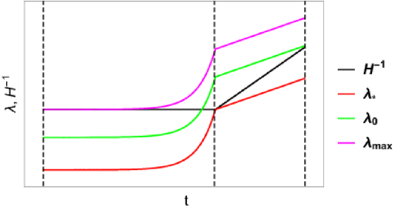
Figure 1: Different scales exit the horizon $H^{-1}$ at different times. We indicate the largest amplified scale, ${\lambda}_{\max}=a/k_{\min}$, the present Hubble scale, ${\lambda}_{0}=a/H_{0}$ and the smallest amplified scale ${\lambda}_{*}$. The dashed vertical lines indicate (from left to right) the beginning of inflation, the end of inflation, and the present time.

This rather simple but fascinating observation is our main result: it implies that a maximally helical scale-invariant magnetic field generated during inflation carries information about the horizon scale at the beginning of inflation. A measurement of ${\cal E}_{\rm M}$ and ${\cal H}_{\rm M}$ allows us to retrieve this information; see Appendix A.

In (2.16), ${\cal E}_{\rm M}$ and ${\cal H}_{\rm M}$ are the values soon after inflation, once the magnetic field is fully helical. Let us now discuss how this ratio changes by subsequent MHD processes within the Hubble horizon. It is well known [107, 108] that the correlation length increases subsequently during the magnetic field decay and that the speed is faster for maximally helical fields. This growth process (within the Hubble horizon) starts shortly after inflation and lasts until recombination. Denoting the reheating temperature after inflation by $T_{\rm f}$, the growth factor for the correlation length for maximally helical fields through the inverse cascade is $(T_{\rm f}/T_{\rm rec})^{p}$. For fully helical fields, one has $p=2/3$, introducing a high inflation scale with for $T_{\rm f}\sim 10^{15}\,{\rm GeV}$ and using $T_{\rm rec}\simeq 0.25\,$eV, the correlation length grows by a factor of the order of $10^{16}$. However, as we shall discuss in the next section, for a scale-invariant magnetic field without subinertial range, we find $p\simeq 0.2\ll 2/3$ and the growth of the correlation length is reduced to a factor $10^{5}$. No theory for the exponent 0.2 is known, and it may not be a universal one, but this is secondary for our present purpose, because uncertainties in the exponent would only yield an additional correction when inferring $k_{\min}$ by determining ${\mathcal{H}}_{\rm M}$ and ${\mathcal{E}}_{\rm M}$ through their effects on the CMB. More precisely,

$$k^{-1}_{\min}\simeq\left(\frac{|{\mathcal{H}}_{\rm M}|}{2{\mathcal{E}}_{\rm M}}\right)_{\rm f}\sim(T_{\rm f}/T_{\rm rec})^{p}\,\frac{|{\mathcal{H}}_{\rm M}|}{2{\mathcal{E}}_{\rm M}}\,.$$ (2.18)

In the case of partially helical fields, there is an additional step. The super-horizon modes retain the initial conditions while the sub-horizon modes are influenced by MHD processes and fields on sub-horizon scales rapidly become maximally helical through magnetic decay while magnetic helicity is conserved. Thus, the ratio $|{\cal H}_{\rm M}|/2{\mathcal{E}}_{\rm M}$ increases until a maximally helical case ($\sigma=1$) is reached. In fact, the MHD processes lead to re-distribution of helicity at large scales and the fractional helicity is a time dependent (growing) function. In this situation, the above equality becomes only a limit, which, in terms of $T_{\rm rec}/T_{\rm f}$, is

$$(T_{\rm rec}/T_{\rm f})^{p}>k_{\min}|{\mathcal{H}}_{\rm M}|/2{\mathcal{E}}_{\rm M}.$$ (2.19)

Thus, for partially helical magnetic fields, we only have $|{\cal H}_{\rm M}|<{\cal H}_{\rm M}^{\max}\equiv 2\xi_{\rm M}{\cal E}_{\rm M}$.

3 Evolution and realizability condition for scale-invariant helical magnetic fields

We now present and discuss results from numerical simulations of the inverse cascade of helical magnetic fields. Numerical simulations show that the well-known inverse cascade of magnetic helicity [109, 110] is strongly reduced if the initial magnetic seed field has a scale-invariant spectrum [101]. Specifically, we have ${\cal E}_{\rm M}\propto t^{p}$ and $\xi_{\rm M}\propto t^{q}$ with $p\approx q\approx 0.2$ instead of $p=q=2/3$, so the correlation length grows much more slowly than for causal fields with $n_{\rm M}=2$. This is not surprising; the smaller the $n_{\rm M}$, the more of the magnetic energy is contained in super-horizon modes which are not affected by plasma processes.

Current limits on the primordial magnetic field from CMB and large-scale structure data are around 1–2 nG; see [113, 112, 111] and references therein. The realizability condition then implies ${\mathcal{H}}_{\rm M}\leq 0.1\,{\rm nG}^{2}\xi_{\rm M}$, and equality is reached for a maximally helical field. As we have already noted above, the correlation length of causally (post-inflation) generated magnetic fields is limited by the Hubble scale $\lambda_{H}$ at the moment of generation,

$$\lambda_{H}=5.8\times 10^{-10}~{}{\rm Mpc}\left(\frac{100\,{\rm GeV}}{T_{\star}}\right)\left(\frac{100}{g_{\star}}\right)^{{1}/{6}},$$ (3.1)

where $T_{\star}$ and $g_{\star}$ are the temperature and number of relativistic degrees of freedom at the generation moment $t_{\star}$ [7]. Accounting for the inverse cascade for maximally helical fields [which increase the correlation length as $(t_{\rm rec}/t_{\star})^{2/3}$, i.e. during the radiation dominated epoch the correlation length increases by $(T_{\star}/0.25~{}{\rm eV})^{2/3}$], the maximal value of the correlation length for the causal field is given by

$$\lambda_{\rm max}\approx 10^{-2}~{}{\rm Mpc}\left(\frac{100\,{\rm GeV}}{T_{\star}}\right)^{1/3}\left(\frac{100}{g_{\star}}\right)^{{1}/{6}},$$ (3.2)

which is substantially smaller than the correlation length of the magnetic field generated during inflation (see Ref. [114] for a recent study on inflationary magnetogenesis).

We construct a random initial magnetic field in Fourier space as

$$B_{i}({\bf k})=B_{0}\left(\delta_{ij}-{\hat{k}}_{i}{\hat{k}}_{j}+i\tilde{\sigma}\epsilon_{ijl}{\hat{k}}_{l}\right)f_{j}({\bf k})\,|{\bf k}|^{n_{\rm M}/2},$$ (3.3)

where ${\bf f}({\bf k})$ is the Fourier transform of a $\delta$-correlated vector field in three dimensions with Gaussian fluctuations, and $n_{\rm M}=-3$ for a scale-invariant spectrum. The degree of helicity is controlled by the parameter $\tilde{\sigma}$ and is given by $\sigma=2\tilde{\sigma}/(1+\tilde{\sigma}^{2})$. We assume $\rho=\rho_{0}={\rm const}$ and ${\bf u}=0$ initially, so the plasma is at rest and the flow is generated from the magnetic field entirely by the Lorentz force.

The full system of equations was derived in Ref. [115] starting from the general relativistic equations in an expanding universe for a flat space-time. We use the ultrarelativistic equation of state where the pressure is given by $p=\rho/3$ and the sound speed is $c_{\rm s}=1/\sqrt{3}$. We assume the bulk velocity ${\bf u}$ to be subrelativistic, so the equations reduce to the usual MHD equations that have frequently been used in the literature [110, 8], except that there are additional $4/3$ factors and some extra terms:

$${\partial\ln\rho\over\partial t} = -\frac{4}{3}\left(\mbox{\boldmath$\nabla$}{}\cdot{\bf u}+{\bf u}\cdot\mbox{\boldmath$\nabla$}{}\ln\rho\right)+{1\over\rho}\left[{\bf u}\cdot({\bf J}\times{\bf B})+\eta{\bf J}^{2}\right]$$ (3.4)

$${\partial{\bf u}\over\partial t} = -{\bf u}\cdot\mbox{\boldmath$\nabla$}{}{\bf u}+{{\bf u}\over 3}\left(\mbox{\boldmath$\nabla$}{}\cdot{\bf u}+{\bf u}\cdot\mbox{\boldmath$\nabla$}{}\ln\rho\right)-{{\bf u}\over\rho}\left[{\bf u}\cdot({\bf J}\times{\bf B})+\eta{\bf J}^{2}\right]$$ (3.6)

$$-{1\over 4}\mbox{\boldmath$\nabla$}{}\ln\rho+{3\over 4\rho}{\bf J}\times{\bf B}+{2\over\rho}\mbox{\boldmath$\nabla$}{}\cdot\left(\rho\nu\mbox{\boldmath${\sf S}$}{}\right)$$

$${\partial{\bf B}\over\partial t} = \nabla\times({\bf u}\times{\bf B}-\eta{\bf J})$$ (3.7)

where ${\sf S}_{ij}={\textstyle{1\over 2}}(u_{i,j}+u_{j,i})-{\textstyle{1\over 3}}\delta_{ij}\mbox{\boldmath$\nabla$}{}\cdot{\bf u}$ is the rate-of-strain tensor, $\nu$ is the viscosity, and $\eta$ is the magnetic diffusivity. The differences compared to the standard MHD equations used in Refs. [110, 8] are minor: the kinetic energy would be overestimated by a factor of 4/3, but the magnetic energy is about the same as for the full set of equations. These differences will be discussed in a separate publication.

Our computational domain has a size $L$, so the smallest wavenumber is given by $k_{0}=2\pi/L$. We adopt a fully or partially helical magnetic field initially with a scale-invariant spectrum $P_{\rm M}(k)\propto k^{-3}$ initially. We define the Alfvén time based on the value of $B_{0}$ with $B_{0}/\rho_{0}^{1/2}c_{\rm s}=0.3$ as $\tau_{\rm A}=(B_{0}k_{0})^{-1}$ and measure conformal time in units of $\tau_{\rm A}$. The rms velocity is $u_{\rm rms}\approx 0.03$ and $\rho_{0}=1$.

We use the Pencil Code [116], which is a public domain code for solving partial differential equations on massively parallel machines. We use a spatial resolution of $1152^{3}$ meshpoints and set $\nu=\eta=5\times 10^{-6}c_{\rm s}/k_{1}$, so the Reynolds number $u_{\rm rms}\xi_{\rm M}/\eta$ is about $10^{4}$. This is large enough so that the precise values of $\nu$ and $\eta$ are not expected to play any role. Moreover, their ratio is taken to be unity, although simulations show that the results still depend on this ratio [117].

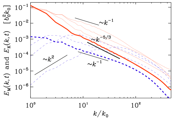
Figure 2: Magnetic (red solid lines) and kinetic (blue dashed lines) energy spectra for $\tilde{\sigma}=\sigma=1$ at times $t/\tau_{\rm A}=0.03$, $0.3$, $1.2$, and $5$. The last time is shown in boldface. For orientation, the $k^{2}$, $k^{-1}$, and $k^{-5/3}$ slopes are indicated.

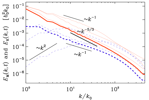
Figure 3: Same as Fig. 2, but for $\tilde{\sigma}=0.03$ ($\sigma\approx 0.06$).

As time goes on, the inflationary helical magnetic field generates helical fluid motions that are characterized by a white noise spectrum, $E_{K}(k)\propto k^{2}$, at large, super-horizon scales, typical of causal fields; see Fig. 2. The magnetic field gets tangled by the resulting velocity field. This leads to a forward cascade of magnetic energy with a slope corresponding to a $k^{-5/3}$ Kolmogorov spectrum at larger wavenumbers. This result is virtually independent of the initial magnetic helicity, as can be seen from the corresponding results for $\tilde{\sigma}=0.03$; see Fig. 3.

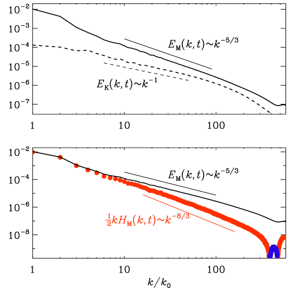
Figure 4: Magnetic and kinetic energy spectra (upper panel) as well as magnetic energy and scaled magnetic helicity spectra (lower panel) for $\sigma=1$ in units of $b_{0}^{2}k_{0}$. Positive (negative) values of $H_{\rm M}(k)$ are indicated by red (blue) symbols.

At the last time of the simulation, the kinetic energy spectrum has approached the magnetic spectrum at small scales, although $E_{\rm K}(k,t)<E_{\rm M}(k,t)$ in all cases. Furthermore, from intermediate $k$ values onward, we find $E_{K}\sim k^{-1}$ and the initial $k^{2}$ subrange has completely disappeared; see the upper panel of Fig. 4. We also compare with magnetic helicity spectra, normalized by $k/2$, which allows us to see how close the realizability condition, ${1\over 2}k|H_{\rm M}(k)|\leq E_{\rm M}(k)$, is to saturation on large scales; see the lower panel of Fig. 4. It turns out that at large scales, where the magnetic field has not yet been affected by the flow, the magnetic field is still nearly fully helical. However, for $k/k_{1}>10$, this is no longer the case and we see that $kH_{\rm M}(k)\sim k^{-8/3}$, i.e., $H_{\rm M}(k)\sim k^{-11/3}$ at sufficiently late times. This behavior has previously also been seen in forced turbulence simulations [108, 118] and is a consequence of a forward cascade of current helicity, $k^{2}H_{\rm M}(k)$, also exhibiting a $k^{-5/3}$ spectrum.

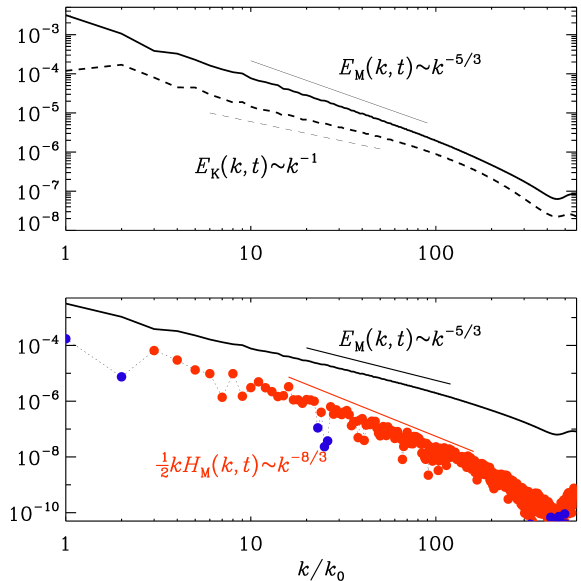
Figure 5: Similar to Fig. 4, but for $\tilde{\sigma}=0.03$ ($\sigma\approx 0.06$).

For $\tilde{\sigma}=0.03$, i.e., $\sigma\approx 0.06$, we find similar characteristics, except that now ${1\over 2}k|H_{\rm M}(k)|\ll E_{\rm M}(k)$; see Fig. 5. There are now also more data points where $H_{\rm M}(k)$ is negative. Nevertheless, we still see a clear $k^{-8/3}$ subrange in $kH_{\rm M}(k)$.

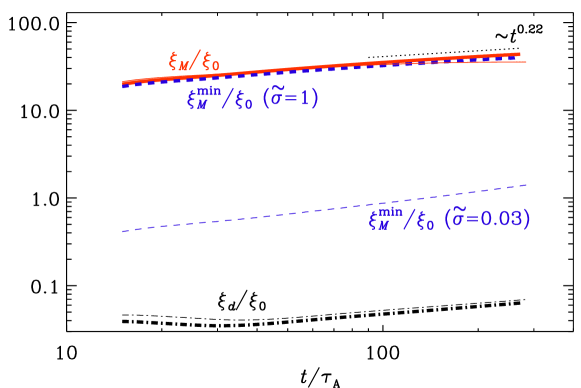
Figure 6: Time evolution of $\xi_{\rm M}=k_{\rm M}^{-1}$ and $\xi_{\rm M}^{\min}$, as well as the Taylor microscale $\xi_{d}$. The thin lines are for $\tilde{\sigma}=0.03$ and the thick ones for $\tilde{\sigma}=1$.

In the present simulations, the initial magnetic energy spectrum had significant energy at large scales, so $\xi_{\rm M}$ is already large initially. Thus, $\xi_{\rm M}$ can only grow owing to the decay of magnetic energy at high wavenumbers. This results in a temporal growth $\xi_{\rm M}\sim t^{0.2}$; see Fig. 6. In the case with $\tilde{\sigma}=0.03$, we find that $\xi_{\rm M}$ first increases and then decreases by a certain amount. This is different from the case of an initial $k^{4}$ subinertial range energy spectrum with fractional helicity, where $\xi_{\rm M}$ is at first growing proportional to $t^{1/2}$. However, as has been demonstrated earlier [14], the growth of $\xi_{\rm M}$ speeds up when it reaches the value $\xi_{\rm M}^{\min}\equiv|{\mathcal{H}}_{\rm M}|/2\xi_{\rm M}{\mathcal{E}}_{\rm M}$, i.e., when the field has become fully helical and thus $\sigma=1$; see Eq. (2.16). In the present case of an initial $k^{-1}$ energy spectrum, $\xi_{\rm M}^{\min}$ also grows (see the dashed line in Fig. 6 for $\tilde{\sigma}=0.03$), but the growth is too slow to become significant.

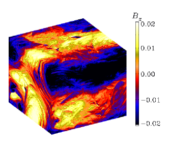
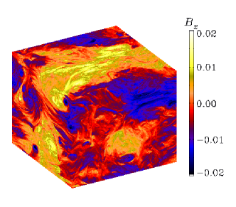
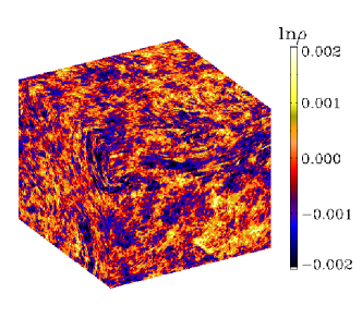
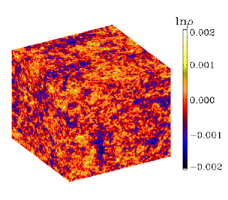
Figure 7: Comparison of $B_{x}$ (upper row) and $\ln\rho$ (lower row) for $\tilde{\sigma}=1$ (left) and $\tilde{\sigma}=0.03$ (right).

Both for $\tilde{\sigma}=1$ and for $\tilde{\sigma}=0.03$, the magnetic field has large-scale structure; see the upper panels of Fig. 7. In some locations, the field appears to have a folded structure with sheets of alternating sign close together. This feature is more pronounced in the case with $\sigma=1$ and reminiscent of similar foldings in forced MHD simulations at large magnetic Prandtl numbers, $\nu/\eta\gg 1$ [119]. In both cases, the effect on the density perturbations is small, but one still sees large-scale patches together with smaller scale structures.

4 Observational consequences

We have discussed scale-invariant helical magnetic fields generated during inflation. We have shown that in the case of a maximally helical magnetic field, the ratio of magnetic helicity and energy densities gives a lower limit of the horizon scale at the beginning of inflation, i.e.,

$$k_{\min}^{-1}\geq\xi_{\rm M}\geq\frac{|{\cal H}_{\rm M}|}{2{\cal E}_{\rm M}}\,.$$ (4.1)

We have found numerically that, while the correlation length grows substantially during the inverse cascade of a causal helical field, this growth is strongly reduced for scale-invariant fields. Consequently, also a fractional helicity $\sigma$ does not grow significantly for scale-invariant helical magnetic fields. Finally, we have argued that it can in principle be measured in the CMB anisotropy and polarization.

The observable signatures of cosmological magnetic helicity and energy density of the magnetic field on large scales have been studied in great detail for the CMB through Faraday rotation (see Ref. [46] and references therein), as well as scalar (density), vector (vorticity), and tensor (gravitational waves) perturbation modes (see Ref. [47] and references therein), and for large-scale structure (see Ref. [113] and references therein). For the helical magnetic fields the most relevant ones are vector [37] and tensor modes [36] of perturbations, since the magnetic helicity is observable through the CMB $B$-polarization that is sourced by the vector and tensor modes. We neglect here the Faraday rotation effect, which is independent of magnetic helicity [43, 44]. We note, however, that, if there is a line-of-sight magnetic field as well as intrinsic polarized emission correlated with the magnetic field, there is in principle the possibility that helical fields can produce a correlation or anti-correlation (depending on the sign of helicity) with the rotation measure [120]. However, this effect could be negligible for inflation-generated fields where $k_{\min}$ is small.

The vector and tensor mode sources are given by the convolution of the magnetic fields (see [37] for the vector mode source and [36] for the tensor mode source, respectively), and as a result, even if the magnetic field is non-vanishing only for $k_{\min}<k<k_{\max}$, the sources are finite also for $k<k_{\min}$. In fact, the infrared white noise amplitude of a typical component of the magnetic energy-momentum tensor is

$$\lim_{{\bf k}\rightarrow 0}\tau_{\mu\nu}({\bf k})\simeq{\cal E}_{\rm M}\,.$$ (4.2)

The helical structure of the source is reflected in the spectral form of the induced perturbations (vorticity and gravitational waves) that have now non-vanishing parity odd correlators (in the case of the tensor mode, magnetic helicity leads to a net circular polarization of gravitational waves) [121].

We define the ratio between the antisymmetric and symmetric parts for vector and tensor modes as ${\mathcal{P}}_{V}$ and ${\mathcal{P}}_{T}$. In the absence of helical magnetic fields (or other parity odd sources) these quantities vanish. Under realistic conditions, the symmetric and antisymmetric parts of the spectra (for both vector and tensor modes) scale differently during the evolution of the universe. We also expect that for a helical source of sufficiently long duration, the induced fluctuations, vorticity or gravitational waves, become maximally helical if the source is maximally helical. Therefore, at late times, ${\mathcal{P}}_{V}(k)\rightarrow 1$ and ${\mathcal{P}}_{T}(k)\rightarrow 1$ for $k\geq k_{H}$, where $k_{H}$ denotes the mode that enters the horizon at time $t$ such that $k_{H}\sim 1/(at)$. The observation of such a parity-odd component of vorticity and gravitational waves from helical magnetic fields in principle allows us to determine both magnetic energy and magnetic helicity densities.

Existing CMB data on the off-diagonal cross-correlations between temperature and $B$-polarization [122, 123, 124] limit the magnetic helicity to roughly 10 nG${}^{2}\,{\rm Gpc}$ [39]. Assuming that the nG limit on magnetic fields [47], $2{\cal E}_{\rm M}\lesssim 0.1$nG², is close to a future detected value, we obtain

$$\left(\frac{|{\cal H}_{\rm M}|}{2{\cal E}_{\rm M}}\right)_{\rm opt}\sim 100\,{\rm Gpc}\,.$$ (4.3)

This is still about 20 times larger than the Hubble scale. Hence, if we were soon to detect a magnetic helicity and energy density close to their present limits, this would represent a very exciting result. However, if we assume a scale-invariant spectrum with a field strength close to the lower limit of $B\gtrsim 10^{-16}\,{\rm G}$, we obtain

$$\left(\frac{|{\cal H}_{\rm M}|}{2{\cal E}_{\rm M}}\right)_{\rm true}\leq 10^{16}\,{\rm Gpc}\,.$$ (4.4)

5 Conclusions

In this work we have shown that a detection of nearly maximal helicity, $|{\cal H}_{\rm M}|\simeq{\cal H}_{\rm M}^{\max}$, can be used to limit the horizon scale at the beginning of inflation,

$$\frac{2{\cal E}_{\rm M}}{|{\cal H}_{\rm M}|}\gtrsim k_{\min}\geq|t|_{\rm in}^{-1}\,.$$ (5.1)

Here, $|t|_{\rm in}\sim(a_{\rm in}H_{\rm in})^{-1}$ is the comoving horizon scale at the beginning of inflation.

This is the first time that a possibility of determining experimentally the beginning of inflation has been proposed. Of course, our method is only applicable if inflation generates not only initial fluctuations for structure formation in the universe but also a scale-invariant spectrum of helical magnetic fields.

Appendix A Monochromatic Magnetic Field

The purpose of this appendix is to illustrate with a simple example how the ratio (2.16) can be measured. For this we consider a monochromatic wave

$${\bf B} = {\bm{\beta}}_{1}\cos({\bf k_{*}\cdot x})+{\bm{\beta}}_{2}\sin({\bf k_{*}\cdot x})$$ (A.1)

$${\bf A} = {\bm{\alpha}}_{1}\sin({\bf k_{*}\cdot x})-{\bm{\alpha}}_{2}\cos({\bf k_{*}\cdot x})$$ (A.2)

where

$${\bm{\beta}}_{i} = {\bf k}_{*}\wedge{\bm{\alpha}}_{i}$$ (A.3)

For simplicity we assume that $\bf k_{*}$ and $\bm{\alpha}_{i}$ are all orthogonal and $|{\bm{\alpha}}_{i}|=\alpha$. The energy density of this field is ${\cal E}_{\rm M}=\frac{1}{2}\langle B^{2}\rangle=k_{*}^{2}(\alpha_{1}^{2}+\alpha_{2}^{2})/4=k_{*}^{2}\alpha^{2}/2$. The helicity is $|{\cal H}_{\rm M}|=|-{\bm{\alpha}}_{1}\cdot{\bm{\beta}}_{2}+{\bm{\alpha}}_{2}\cdot{\bm{\beta}}_{1}|/2=k_{*}\alpha^{2}$. Hence, for this (maximally helical) case

$$\frac{|{\cal H}_{\rm M}|}{2{\cal E}_{\rm M}}=k_{*}^{-1}\,.$$ (A.4)

This example is of course not very realistic as an average over many wavelengths is required. In the cosmological context we perform ensemble averages which, perhaps, are best compared with averaging ${\cal E}_{\rm M}$ and ${\cal H}_{\rm M}$ over many phases.

$Header: /var/cvs/brandenb/tex/tina/inflation-hel/paper.tex,v 1.85 2017/11/22 20:08:06 brandenb Exp $

References

- [1] L. M. Widrow, Rev. Mod. Phys. 74, 775 (2002) [astro-ph/0207240].
- [2] A. Neronov and I. Vovk, Science 328, 73 (2010) [arXiv:1006.3504 [astro-ph.HE]].
- [3] A. Taylor, I. Vovk and A. Neronov, Astron. & Astrophys. 529, 144 (2011) [arXiv:1101.0932].
- [4] R. M. Kulsrud and E. G. Zweibel, Rept. Prog. Phys. 71, 0046091 (2008) [arXiv:0707.2783 [astro-ph]].
- [5] A. Kandus, K. E. Kunze and C. G. Tsagas, Phys. Rept. 505, 1 (2011) [arXiv:1007.3891 [astro-ph.CO]].
- [6] R. Durrer and A. Neronov, Astron. Astrophys. Rev 21, 62 (2013) [arXiv:1303.7121 [astro-ph.CO]].
- [7] T. Kahniashvili, A. G. Tevzadze, A. Brandenburg and A. Neronov, Phys. Rev. D 87, 083007 (2013) [arXiv:1212.0596 [astro-ph.CO]].
- [8] R. Banerjee and K. Jedamzik, Phys. Rev. D 70, 123003 (2004) [arXiv:astro-ph/0410032].
- [9] T. C. Ching, S. P. Lai, Q. Zhang, L. Yang, J. M. Girart, and R. Rao, Astrophys. J. 819, 159 (2016) [arXiv:1601.05229[astro-ph]].
- [10] T. A. Enßlin, Astron. Astrophys. 401, 499 (2003) [astro-ph/0212387].
- [11] H. Tashiro and T. Vachaspati, Mon. Not. Roy. Astron. Soc. 448, 299 (2015) [arXiv:1409.3627 [astro-ph.CO]].
- [12] W. Chen, B. D. Chowdhury, F. Ferrer, H. Tashiro and T. Vachaspati, Mon. Not. Roy. Astron. Soc. 450, 3371 (2015) [arXiv:1412.3171 [astro-ph.CO]].
- [13] D. Biskamp and W.-C. Müller, Phys. Rev. Lett. 83, 2195 (1999).
- [14] A. G. Tevzadze, L. Kisslinger, A. Brandenburg and T. Kahniashvili, Astrophys. J. 759, 54 (2012) [arXiv:1207.0751 [astro-ph.CO]].
- [15] A. J. Long, E. Sabancilar and T. Vachaspati, JCAP 1402, 036 (2014) [arXiv:1309.2315 [astro-ph.CO]].
- [16] T. Fujita and K. Kamada, Phys. Rev. D 93, 083520 (2016) [arXiv:1602.02109 [hep-ph]].
- [17] J. M. Cornwall, Phys. Rev. D 56, 6146 (1997) [arXiv:hep-th/9704022].
- [18] M. Giovannini and M. E. Shaposhnikov, Phys. Rev. D 57, 2186 (1998) [arXiv:hep-ph/9710234].
- [19] G. B. Field and S. M. Carroll, Phys. Rev. D 62, 103008 (2000) [arXiv:astro-ph/9811206].
- [20] T. Vachaspati, Phys. Rev. Lett. 87, 251302 (2001) [arXiv:astro-ph/0101261].
- [21] H. Tashiro, T. Vachaspati and A. Vilenkin, Phys. Rev. D 86, 105033 (2012) [arXiv:1206.5549 [astro-ph.CO]].
- [22] G. Sigl, Phys. Rev. D 66, 123002 (2002) [arXiv:astro-ph/0202424].
- [23] K. Subramanian and A. Brandenburg, Phys. Rev. Lett. 93, 205001 (2004) [arXiv:astro-ph/0408020].
- [24] L. Campanelli and M. Giannotti, Phys. Rev. D 72, 123001 (2005) [arXiv:astro-ph/0508653].
- [25] V. B. Semikoz and D. D. Sokoloff, Astron. Astrophys. 433, L53 (2005) [astro-ph/0411496]; Int. J. Mod. Phys. D 14, 1839 (2005).
- [26] A. Diaz-Gil, J. Garcia-Bellido, M. Garcia Perez and A. Gonzalez-Arroyo, Phys. Rev. Lett. 100, 241301 (2008) [arXiv:0712.4263 [hep-ph]].
- [27] L. Campanelli, Int. J. Mod. Phys. D 18, 1395 (2009) [arXiv:0805.0575 [astro-ph]].
- [28] L. Campanelli, Phys. Rev. Lett. 111, 061301 (2013) [arXiv:1304.6534 [astro-ph.CO]].
- [29] R. K. Jain, R. Durrer and L. Hollenstein, J. Phys. Conf. Ser. 484, 012062 (2014) [arXiv:1204.2409 [astro-ph.CO]].
- [30] A. Boyarsky, J. Frohlich and O. Ruchayskiy, Phys. Rev. Lett. 108, 031301 (2012) [arXiv:1109.3350 [astro-ph.CO]].
- [31] C. Caprini and L. Sorbo, JCAP 1410, 056 (2014) [arXiv:1407.2809 [astro-ph.CO]].
- [32] E. Calzetta and A. Kandus, Phys. Rev. D 89, 083012 (2014) [arXiv:1403.1193 [astro-ph.CO]].
- [33] E. F. Piratova, E. A. Reyes and H. J. Hortua, arXiv:1409.1567 [astro-ph.CO].
- [34] J. M. Wagstaff and R. Banerjee, JCAP 1601, 002 (2016) [arXiv:1409.4223 [astro-ph.CO]].
- [35] L. Pogosian, T. Vachaspati and S. Winitzki, Phys. Rev. D 65, 083502 (2002) [astro-ph/0112536].
- [36] C. Caprini, R. Durrer and T. Kahniashvili, Phys. Rev. D 69, 063006 (2004) [arXiv:astro-ph/0304556].
- [37] T. Kahniashvili and B. Ratra, Phys. Rev. D 71, 103006 (2005) [arXiv:astro-ph/0503709].
- [38] K. E. Kunze, Phys. Rev. D 85, 083004 (2012) [arXiv:1112.4797 [astro-ph.CO]].
- [39] T. Kahniashvili, Y. Maravin, G. Lavrelashvili and A. Kosowsky, Phys. Rev. D 90, 083004 (2014) [arXiv:1408.0351 [astro-ph.CO]].
- [40] M. Ballardini, F. Finelli and D. Paoletti, JCAP 1510, 031 (2015) [arXiv:1412.1836 [astro-ph.CO]].
- [41] A. Kosowsky and A. Loeb, Astrophys. J. 469, 1 (1996) [astro-ph/9601055].
- [42] T. A. Ensslin and C. Vogt, Astron. Astrophys. 401, 835 (2003) [arXiv:astro-ph/0302426].
- [43] L. Campanelli, A. D. Dolgov, M. Giannotti and F. L. Villante, Astrophys. J. 616, 1 (2004) [astro-ph/0405420].
- [44] A. Kosowsky, T. Kahniashvili, G. Lavrelashvili and B. Ratra, Phys. Rev. D 71, 043006 (2005) [astro-ph/0409767].
- [45] T. Kahniashvili, Y. Maravin and A. Kosowsky, Phys. Rev. D 80, 023009 (2009) [arXiv:0806.1876 [astro-ph]].
- [46] P. A. R. Ade et al. [POLARBEAR Collaboration], Phys. Rev. D 92, 123509 (2015) [arXiv:1509.02461 [astro-ph.CO]].
- [47] P. A. R. Ade et al. [Planck Collaboration], Astron. Astrophys. 594, A19 (2016) [arXiv:1502.01594 [astro-ph.CO]].
- [48] P. Cabella, P. Natoli and J. Silk, Phys. Rev. D 76, 123014 (2007) [arXiv:0705.0810 [astro-ph]].
- [49] J. Q. Xia, H. Li, X. l. Wang and X. m. Zhang, arXiv:0710.3325 [hep-ph].
- [50] B. Feng, M. Li, J. Q. Xia, X. Chen and X. Zhang, Phys. Rev. Lett. 96, 221302 (2006) [arXiv:astro-ph/0601095].
- [51] J. -Q. Xia, JCAP 1201, 046 (2012) [arXiv:1201.4457 [astro-ph.CO]].
- [52] J. -Q. Xia, H. Li and X. Zhang, Phys. Lett. B 687, 129 (2010) [arXiv:0908.1876 [astro-ph.CO]].
- [53] M. Li, Y. -F. Cai, X. Wang and X. Zhang, Phys. Lett. B 680, 118 (2009) [arXiv:0907.5159 [hep-ph]].
- [54] M. Li and X. Zhang, Rev. D 78, 103516 (2008) [arXiv:0810.0403 [astro-ph]].
- [55] A. Gruppuso, P. Natoli, N. Mandolesi, A. De Rosa, F. Finelli and F. Paci, JCAP 1202, 023 (2012) [arXiv:1107.5548 [astro-ph.CO]].
- [56] G. Gubitosi and F. Paci, JCAP 1302, 020 (2013) [arXiv:1211.3321 [astro-ph.CO]].
- [57] M. Li and B. Yu, JCAP 1306, 016 (2013) [arXiv:1303.1881 [astro-ph.CO]].
- [58] V. Gluscevic, D. Hanson, M. Kamionkowski and C. M. Hirata, Phys. Rev. D 86, 103529 (2012) [arXiv:1206.5546 [astro-ph.CO]].
- [59] A. Ben-David and E. D. Kovetz, Mon. Not. Roy. Astron. Soc. 445, 2116 (2014) [arXiv:1403.2104 [astro-ph.CO]].
- [60] J. D. Tasson, Rept. Prog. Phys. 77, 062901 (2014) [arXiv:1403.7785 [hep-ph]].
- [61] J. Kaufman, B. Keating and B. Johnson, Mon. Not. Roy. Astron. Soc. 455, 1981 (2016) [arXiv:1409.8242 [astro-ph.CO]].
- [62] A. Lue, L. M. Wang and M. Kamionkowski, Phys. Rev. Lett. 83, 1506 (1999) [arXiv:astro-ph/9812088].
- [63] J. Q. Xia, H. Li, G. B. Zhao and X. Zhang, arXiv:0803.2350 [astro-ph].
- [64] S. Saito, K. Ichiki and A. Taruya, JCAP 0709, 002 (2007) [arXiv:0705.3701 [astro-ph]].
- [65] E. S. Scannapieco and P. G. Ferreira, Phys. Rev. D 56, 7493 (1997) [arXiv:astro-ph/9707115].
- [66] C. Scoccola, D. Harari and S. Mollerach, Phys. Rev. D 70, 063003 (2004) [arXiv:astro-ph/0405396].
- [67] M. Demianski and A. G. Doroshkevich, Phys. Rev. D 75, 123517 (2007) [arXiv:astro-ph/0702381].
- [68] J. R. Kristiansen and P. G. Ferreira, Phys. Rev. D 77, 123004 (2008) [arXiv:0803.3210 [astro-ph]].
- [69] J. Adamek, R. Durrer, E. Fenu and M. Vonlanthen, JCAP 1106 (2011) 017 [arXiv:1102.5235 [astro-ph.CO]].
- [70] S. M. Carroll, G. B. Field and R. Jackiw, Phys. Rev. D 41, 1231 (1990).
- [71] V. A. Kostelecky and M. Mewes, Phys. Rev. Lett. 99, 011601 (2007) [arXiv:astro-ph/0702379].
- [72] Y. -F. Cai, M. Li and X. Zhang, JCAP 1001, 017 (2010) [arXiv:0912.3317 [hep-ph]].
- [73] W. -T. Ni, Prog. Theor. Phys. Suppl. 172, 49 (2008) [arXiv:0712.4082 [astro-ph]].
- [74] R. Casana, M. M. Ferreira, Jr. and J. S. Rodrigues, Phys. Rev. D 78, 125013 (2008) [arXiv:0810.0306 [hep-th]].
- [75] R. R. Caldwell, V. Gluscevic and M. Kamionkowski, Phys. Rev. D 84, 043504 (2011) [arXiv:1104.1634 [astro-ph.CO]].
- [76] H. J. Mosquera Cuesta and G. Lambiase, JCAP 1103, 033 (2011) [arXiv:1102.3092 [astro-ph.CO]].
- [77] M. Kamionkowski and T. Souradeep, Phys. Rev. D 83, 027301 (2011) [arXiv:1010.4304 [astro-ph.CO]].
- [78] V. Gluscevic and M. Kamionkowski, Phys. Rev. D 81, 123529 (2010) [arXiv:1002.1308 [astro-ph.CO]].
- [79] M. Mewes, Phys. Rev. D 85, 116012 (2012) [arXiv:1203.5331 [hep-ph]].
- [80] W. -T. Ni, arXiv:0910.4317 [gr-qc].
- [81] N. J. Miller, M. Shimon and B. G. Keating, Phys. Rev. D 79, 103002 (2009) [arXiv:0903.1116 [astro-ph.CO]].
- [82] W. -T. Ni, Int. J. Mod. Phys. A 24, 3493 (2009) [arXiv:0903.0756 [astro-ph.CO]].
- [83] E. A. Lim, Phys. Rev. D 71, 063504 (2005) [arXiv:astro-ph/0407437].
- [84] S. M. Carroll and E. A. Lim, Phys. Rev. D 70, 123525 (2004) [arXiv:hep-th/0407149].
- [85] S. H. S. Alexander, Phys. Lett. B 660, 444 (2008) [arXiv:hep-th/0601034].
- [86] M. Satoh, S. Kanno and J. Soda, Phys. Rev. D 77, 023526 (2008) [arXiv:0706.3585 [astro-ph]].
- [87] A. Gruppuso, M. Gerbino, P. Natoli, L. Pagano, N. Mandolesi, A. Melchiorri and D. Molinari, JCAP 1606, 001 (2016) [arXiv:1509.04157 [astro-ph.CO]].
- [88] T. Kahniashvili and B. Ratra, Phys. Rev. D 75, 023002 (2007) [astro-ph/0611247].
- [89] K. Subramanian, Rept. Prog. Phys. 79, 076901 (2016) [arXiv:1504.02311 [astro-ph.CO]].
- [90] M. M. Anber and L. Sorbo, JCAP 0610, 018 (2006) [astro-ph/0606534].
- [91] R. Durrer, L. Hollenstein and R. K. Jain, JCAP 1103, 037 (2011) [arXiv:1005.5322 [astro-ph.CO]].
- [92] C. Bonvin, C. Caprini and R. Durrer, Phys. Rev. D 86, 023519 (2012) [arXiv:1112.3901 [astro-ph.CO]].
- [93] B. Ratra, Astrophys. J. 391, L1 (1992).
- [94] B. Ratra, Caltech preprint GRP-287/CALT-68-1751 (1991) available at www.phys.ksu.edupersonalratra.
- [95] V. Demozzi, V. Mukhanov and H. Rubinstein, JCAP 0908, 025 (2009) [arXiv:0907.1030 [astro-ph.CO]].
- [96] S. Kanno, J. Soda and M.-a. Watanabe, JCAP 0912, 009 (2009) [arXiv:0908.3509 [astro-ph.CO]].
- [97] R. Emami, H. Firouzjahi and M. S. Movahed, Phys. Rev. D 81, 083526 (2010) [arXiv:0908.4161 [hep-th]].
- [98] V. Demozzi and C. Ringeval, JCAP 1205, 009 (2012) [arXiv:1202.3022 [astro-ph.CO]].
- [99] L. Motta and R. R. Caldwell, Phys. Rev. D 85, 103532 (2012) [arXiv:1203.1033 [astro-ph.CO]].
- [100] T. Kahniashvili, A. Brandenburg, L. Campanelli, B. Ratra and A. G. Tevzadze, Phys. Rev. D 86, 103005 (2012) [arXiv:1206.2428 [astro-ph.CO]].
- [101] A. Brandenburg and T. Kahniashvili, Phys. Rev. Lett. 118, 055102 (2017) [arXiv:1607.01360 [physics.flu-dyn]].
- [102] M. A. Berger, Plasma Physics and Controlled Fusion 41 167 (1999).
- [103] A. Brandenburg, R. Durrer, T. Kahniashvili, S. Mandal, A. Tevzadze, W. Yin, 2017, in preparation.
- [104] R. Durrer and C. Caprini, JCAP 0311, 010 (2003) [arXiv:astro-ph/0305059].
- [105] A. S. Monin and A. M. Yaglom, Statistical Fluid Mechanics, MIT Press, Cambridge, MA, (1975).
- [106] P. A. R. Ade et al. [Planck Collaboration], Astron. Astrophys. 594, A20 (2016) [arXiv:1502.02114 [astro-ph.CO]].
- [107] U. Frisch, A. Pouquet, J. Léorat, and A. Mazure, J. Fluid Mech. 68, 769 (1975).
- [108] A. Brandenburg and K. Subramanian, Astron. Astrophys. 439, 835 (2005) [astro-ph/0504222].
- [109] A. Pouquet, U. Frisch and J. Leorat, J. Fluid Mech. 77, 321 (1976).
- [110] M. Christensson, M. Hindmarsh and A. Brandenburg, Phys. Rev. E 64, 056405 (2001) [astro-ph/0011321].
- [111] P. A. R. Ade et al. [Planck Collaboration], Astron. Astrophys. 571, A16 (2014) [arXiv:1303.5076 [astro-ph.CO]].
- [112] D. G. Yamazaki, K. Ichiki and K. Takahashi, Phys. Rev. D 88, 103011 (2013) [arXiv:1311.2584 [astro-ph.CO]].
- [113] T. Kahniashvili, Y. Maravin, A. Natarajan, N. Battaglia and A. G. Tevzadze, Astrophys. J. 770, 47 (2013) [arXiv:1211.2769 [astro-ph.CO]].
- [114] R. Sharma, S. Jagannathan, T. R. Seshadri and K. Subramanian, arXiv:1708.08119 [astro-ph.CO].
- [115] A. Brandenburg, K. Enqvist and P. Olesen, Phys. Rev. D 54, 1291 (1996) [astro-ph/9602031].
- [116] http://github.com/pencil-code/
- [117] A. Brandenburg, , Astrophys. J. 791, 12 (2014). [arXiv:1404.6964 [astro-ph]].
- [118] A. Brandenburg, Astrophys. J. 697, 1206 (2009) [arXiv:0808.0961 [astro-ph]].
- [119] A. A. Schekochihin, S. C. Cowley, S. F. Taylor, J. L. Maron and J. C. McWilliams, Astrophys. J. 612, 276 (2004) [astro-ph/0312046].
- [120] A. Brandenburg and R. Stepanov, Astrophys. J. 786, 91 (2014) [arXiv:1401.4102 [astro-ph.CO]].
- [121] T. Kahniashvili, G. Gogoberidze and B. Ratra, Phys. Rev. Lett. 100, 231301 (2008) [arXiv:0802.3524 [astro-ph]].
- [122] C. L. Bennett et al. [WMAP Collaboration], Astrophys. J. Suppl. 208, 20 (2013) [arXiv:1212.5225 [astro-ph.CO]];
- [123] G. Hinshaw et al. [WMAP Collaboration], Astrophys. J. Suppl. 208, 19 (2013) [arXiv:1212.5226 [astro-ph.CO]].
- [124] D. Larson, J. Dunkley, G. Hinshaw, E. Komatsu, M. R. Nolta, C. L. Bennett, B. Gold and M. Halpern et al., Astrophys. J. Suppl. 192, 16 (2011) [arXiv:1001.4635 [astro-ph.CO]].