Superfluid filaments of dipolar bosons in free space

Abstract

We systematically investigate the zero temperature phase diagram of bosons interacting via dipolar interactions in three dimensions in free space via path integral Monte Carlo simulations with few hundreds of particles and periodic boundary conditions based on the worm algorithm. Upon increasing the strength of the dipolar interaction and at sufficiently high densities we find a wide region where filaments are stabilized along the direction of the external field. Most interestingly by computing the superfluid fraction we conclude that superfluidity is anisotropic and is greatly suppressed along the orthogonal plane. Finally we perform simulations at finite temperature confirming the stability of filaments against thermal fluctuations and provide an estimate of the superfluid fraction in the weak coupling limit in the framework of the Landau two-fluid model.

Superfluidity is an amazing phenomenon of quantum mechanical origin that manifests itself macroscopically as frictionless flow and lack of response to rotation for small enough angular velocity pitaevskii2003 ; pethick2002 . Several experimental platforms have been used to investigate quantum matter in the superfluid regime leggett2006 . Among them, ultracold gases realize a very clean and controllable many-body playground that permit the observation of quantum properties with unprecedented precision bloch2008 . In these systems superfluidity has been observed both with bosonic as well as with fermionic atoms verney2015 ; tey2013 ; pitaevskii2015 ; hou2013 . The superfluid fraction, the ratio of the superfluid density to the total density of the system, has been recently measured in two-component Fermi gas interacting via strong contact potentials pitaevskii2015 ; salasnich2010 ; sidorenkov2013 .

An even richer phenomenology appears when long-range interactions are present. The non-local character of the interparticle potential may induce instabilities of the density that lead to a spontaneous breaking of translational symmetry. A primary example is the long sought supersolid state, where superfluidity is accompanied by a crystalline order boninsegni2012 ; cinti2014 ; leonard2017 ; li2017 . Recent groundbreaking experiments with dipolar condensates demonstrated the existence of dense bosonic droplets in trapped configurations kadau2016 ; ferrier2016 ; chomaz2016 ; ferrier2016-jpb and in free space schmitt2016 . Beyond mean-field effects wachtler2016 ; bisset2016 ; baillie2016 and three-body interactions bisset2015 have been invoked as the main mechanisms responsible for the stability of these clusters. Large scale simulations based on a non-local non-linear Schrödinger equation have shown very good agreement with the density distribution and the excitation spectra observed in laboratory. Latest experiments paved the way for the search of phase coherence of droplets, demonstrating interference pattern via expansion dynamics of the condensate. The presence of fringes showed that each droplet is individually phase coherent and thus superfluid, leaving yet unresolved the question of global phase coherence of the system ferrier2016 .

In this Letter we report path-integral Monte Carlo (PIMC) results for the low temperature properties of a finite size system of dipolar bosons in three dimensional free space. Recent works showed with similar methods the existence of a window in parameter space leading to stable self-bound configurations of a single saito2016 or several droplets in a regular arrangement in trapped configurations macia2016 . Yet, no work has investigated the superfluid character of these structures. Here we address the issue of superfluidity for a wide range of the strength of the dipolar interaction and density as well as their stability against finite temperature fluctuations. We carry out large scale simulations, based on a continuous-space worm algorithm which allows for an efficient and reliable determination of the superfluid density boninsegni2006 ; boninsegni2006-pre . We observe an anisotropic character of the superfluid fraction in the inhomogeneous regime of the filaments. Our results are consistent with the absence of supersolidity in these systems.

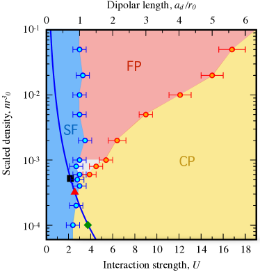
Figure 1: Zero-temperature phases of dipolar bosons in three dimensions in free space: Superfluid (SF), superfluid filaments (FP) and cluster phases (CP) for varying dimensionless interaction strength $U$ (or equivalently dipolar length $a_{d}/r_{0}$) and scaled density $nr_{0}^{3}$. For $a_{d}/r_{0}\lesssim 0.9$ the blue SF region corresponds to a uniform superfluid, which agrees with mean-field prediction that predicts stability for $a_{d}/a_{s}<1$. FP is encountered for high densities $nr_{0}^{3}\gtrsim 5\cdot 10^{-4}$ and for $a_{d}/r_{0}\gtrsim 1$. For small densities $nr_{0}^{3}\lesssim 5\cdot 10^{-4}$ the system breaks up into tiny clusters. Phase boundaries in the grey region are not resolved. Blue line corresponds to $n=5\cdot 10^{20}\,$m^-3 and $a_{d}=130\,a_{0}$. Black/Red dots are experimentally measured background scattering lengths $a_{s}=122\,a_{0}$ (¹⁶²Dy) / $a_{s}=92\,a_{0}$ (¹⁶⁴Dy). Green point at $a_{s}=29\,a_{0}$ nota3 .

The Hamiltonian of an ensemble of $N$ interacting identical bosons is:

$$\hat{H}=-\sum_{i=1}^{N}\frac{\hbar^{2}}{2m}\nabla_{i}^{2}+\sum_{i<j}^{N}V(\mathbf{r}_{i}-\mathbf{r}_{j}),$$ (1)

where $m$ is the particle mass, $\mathbf{r}_{i}$ is the position of the $i$-th dipole. We model the interparticle potential $V(\bf{r})$ by a short-range hard-core with cutoff $r_{0}$ and an anisotropic long-range dipolar potential:

$$V(\mathbf{r})=\left\{\begin{array}[]{cc}\frac{C_{dd}}{4\pi}\frac{1-3\cos^{2}\theta}{r^{3}}&\text{if}~{}r\geq r_{0},\\ \infty&\text{if}~{}r<r_{0},\end{array}\right.$$ (2)

where $C_{dd}/4\pi$ is the coupling constant and the angle $\theta$ denotes the angle between the vector $\bf{r}$ and the $z$-axis. Here the units of length and energy are $r_{0}$ and $\hbar^{2}/mr_{0}^{2}$, respectively. Therefore the zero-temperature physics is controlled by the dimensionless interaction strength $U=mC_{dd}/4\pi\hbar^{2}r_{0}$ and the dimensionless density $nr_{0}^{3}$ only nota1 . Eq.(1) applies both to vertically aligned dipoles interacting via magnetic or electric dipole moments lahaye2009 . The hard-core with radius $r_{0}$ removes the unphysical $1/r^{3}$ attraction of dipoles in head-to-tail configurations at small distances. Finite dipolar potentials affect the scattering length $a_{s}$ associated to the contact potential into a non-trivial relation of $C_{dd}$ bortolotti2006 ; ronen2006 ; jachymski2016 . This turns out to be crucial to account for the stability properties of a dipolar gas in generic (beyond) mean-field approaches. For example a standard Bogoliubov calculation determines the stability of a homogeneous condensate when $\epsilon_{d}\equiv a_{d}/a_{s}<1$ is satisfied, where $a_{d}=\frac{C_{dd}m}{12\pi\hbar^{2}}$ is the dipolar length associated to Eq.(2) lahaye2009 ; baranov2012 .

We determine the equilibrium properties of Eq. (1) in a wide range of scaled average density $nr_{0}^{3}$ (different from experimentally measured peak density) and interaction strength $U$. We work with $N$ atoms in a cubic box of linear dimension $L$ and periodic boundary conditions. At fixed density $n=N/L^{3}$, with $N=100-400$, we verified that the phase diagram does not change. Thus, our finite-size results give a reasonable estimate of thermodynamic limit. nota2 . From these simulations we obtain, for example, density profiles, and radial correlation functions, as well as the superfluid fraction svistunov2015 at finite temperatures. The phases were obtained by extrapolating to the limit of zero temperature, lowering the temperature until observables, such as the total energy, superfluid fraction $f_{s}$ and radial correlations did not change on further decrease of $T$. These observables were then analyzed to construct the phase diagram in Fig.1.

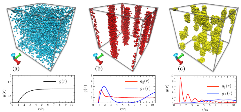
Figure 2: Characterization of the phases at $nr_{0}^{3}=10^{-2}$. Upper panels. PIMC density distribution at different strengths of dipolar interaction: (a) SF at $a_{d}=0.6r_{0}$, (b) superfluid FP at $a_{d}=2.6r_{0}$ and (c) CP at $a_{d}=6.0r_{0}$. Lower panels. (a) radial correlation functions $g(r)$ in the SF. (b) and (c) radial correlation functions $g_{\parallel}(r)$ along the vertical direction (red) and $g_{\perp}(r)$ along the orthogonal plane (blue). $g_{\parallel}(r)$ has a fluid-like profile in the FP. In the CP $g_{\parallel}(r)$ a high peak due to strong attractive interactions appears at distances $r\gtrsim r_{0}$. $g_{\perp}(r)$ in the FP shows a strong suppression in between two filaments whereas in the CP it flattens at intermediate distances. Simulations are done with $100$ particles and $500$ slices. Correlation functions are averaged over $100$ configurations.

For small $U$ the system is in a superfluid phase (SF) with unitary $f_{s}$. For low densities $n\,r_{0}^{3}\lesssim 10^{-3}$ the SF extends up to $U\approx 2.1$ which agrees with the mean-field phase boundary predicted by standard Bogoliubov analysis ($\epsilon_{d}=1$) for the dipolar potential and a contact interaction nota3 . Increasing the interaction strength the system enters into a cluster phase (CP) with vanishing superfluidity and characterized by droplet structures with few particles. For higher densities $nr_{0}^{3}>6\cdot 10^{-4}$, crossing the SF phase boundary, we encounter a phase characterized by elongated filaments (FP) with anisotropic superfluid fraction. We notice that this FP extends from small positive induced contact potential ($\epsilon_{d}\gtrsim 1$) which corresponds to the experimentally relevant regime of kadau2016 ; nota3 ; yi2000 ; yi2001 ; tang2015 ; maier2015 ; burdick2016 ; chaikin1995 , to the strongly coupled limit of large dipolar interactions and large densities. For intermediate densities $6\cdot 10^{-4}\lesssim n\,r_{0}^{3}\lesssim 1\cdot 10^{-3}$ the phase boundaries are not resolved.

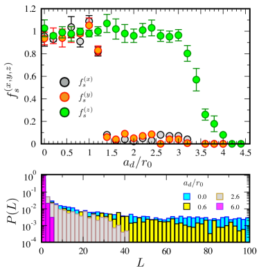
Figure 3: Superfluid fraction $f_{s}$ across the transition from superfluid to filament transition at high densities. Upper panel. $f_{s}$ as a function of the dipolar length along the vertical direction and the orthogonal direction for $nr_{0}^{3}=10^{-2}$. Dipoles and filaments are aligned along the $z$-axis. In the SF the superfluid fraction converges to $f_{s}=1$ isotropically. In the filaments we observe $f_{s}=1$ along the vertical axis and vanishing on the orthogonal plane. Error bars are statistical uncertainties. Lower panel. Relative frequency of permutation cycles of length $L$ again for $nr_{0}^{3}=10^{-2}$ and $a_{d}=0,0.6,2.8,6.0\,r_{0}$ in the the SF (blue and yellow), FP (grey) and CP (purple).

Representative PIMC configurations with $100$ particles and $500$ imaginary-time slices ($n\,r_{0}^{3}=10^{-2}$) of the density distribution are shown in Fig.2. In the SF (Fig.2a) particles delocalize into a phase with uniform density displaying flat radial distribution functions, $g(r)$, typical of a fluid phase of particles interacting via hard-core potentials. In Fig.2b a typical configuration of the FP is illustrated where filaments elongate vertically. Finally in the CP several small clusters form, slightly elongated along the vertical direction, signaling a fragmentation of the filaments for large interactions. In the non-homogeneous FP and CP we analyze $g(r)$ along two orthogonal directions. The function $g_{\parallel}(r)$ (red line in Fig.2) is computed along the vertical axis parallel to the direction of the filaments. In the FP $g_{\parallel}(r)$ has a liquid-like profile with a peak $r\gtrsim r_{0}$ as a consequence of the attractive part of the dipolar interaction and the large density along the $z$-axis. In the CP the first peak of $g_{\parallel}(r)$ is higher and the function oscillates several times before vanishing for large distances as a consequence of the finite size of the clusters. The correlation $g_{\perp}(r)$ (blue line) is evaluated along the horizontal plane, perpendicular to the direction of the filaments. In the FP, it is strongly suppressed in the region between two filaments. In the CP $g_{\perp}(r)$ flattens at intermediate distances displaying an irregular arrangement of the small dipolar droplets along the horizontal plane.

To fully characterize the genuine quantum properties of the FP we compute the superfluid fraction $f_{s}^{(i)}$ as a function of the interaction strength and temperature along three orthogonal directions $i=\,x,\,y,z$, yielding $f_{s}^{(i)}=\frac{mk_{B}T}{\hbar^{2}\,n}\langle w_{i}^{2}\rangle$, where $\langle\ldots\rangle$ stands for the thermal average of the winding number estimator $w_{i}$ pollock1987 ; ceperley1995 . Fig.3 depicts the superfluid fraction $f_{s}^{(i)}$ calculated varying the dipolar length $a_{d}$ for $nr_{0}^{3}=10^{-2}$. In the SF the superfluid density is uniform and unitary ($f_{s}^{(i)}=1$). Crossing the SF-FP phase boundary $f_{s}^{(i)}$ displays a strong anisotropy. The superfluid fraction is unitary along the vertical direction and it is greatly suppressed along the orthogonal $x-y$ plane, showing only a marginal finite-size effect contribution to $w_{x}$ and $w_{y}$, respectively. This result suggests that each filament is phase coherent, but globally the system is not. This suppression of superfluidity along two directions resembles the formation of a sliding phase in weakly-coupled superfluid layers in the thermodynamic limit ohern99 ; pekker10 ; laflorencie12 ; vayl17 . Finally entering in the CP $f_{s}^{(i)}=0$ uniformly as expected from the fragmentation of the filaments in the configurations. The lower panel of Fig.3 reports the relative frequency of exchange cycles involving a particle number $1\leq L\leq N$ jain2011 . In the SF we observe long permutation cycles ($\sim N$). In the FP (CP) cycles reduce to few tens of (few) particles in support of the previous observation that superfluidity originates within each filament (locally within each cluster).

Finally we investigate the stability of superfluid filaments at finite temperatures. In Fig.4 we show the superfluid fraction for a system of $N=100$ particles at density $nr_{0}^{3}=10^{-2}$ as a function of $T/T_{0}$, $T_{0}$ being the critical temperature of an ideal Bose gas $k_{B}T_{0}=\frac{2\pi}{\zeta\left(3/2\right)^{2/3}}\left(nr_{0}^{3}\right)^{2/3}$ nota4 . In the SF we compare PIMC results with an analytical calculation within the Landau two-fluid model ghabour2014

$$f_{s}^{(z)}=1-\frac{\beta\hbar^{2}}{4\pi^{2}m}\int_{0}^{\infty}dq\int_{0}^{\pi}d\theta_{q}q^{4}\frac{\sin\theta_{q}\cos^{2}\theta_{q}e^{\beta E_{q}}}{(e^{\beta E_{q}}-1)^{2}}$$ (3)

where $E_{\mathbf{q}}$=$\sqrt{\frac{\hbar^{2}q^{2}}{2m}\left(\frac{\hbar^{2}q^{2}}{2m}+2\frac{\mu}{g_{0}}\tilde{V}_{\text{ps}}(\mathbf{q})\right)}$ is the Bogoliubov spectrum. The function $\tilde{V}_{\text{ps}}(\mathbf{q})=g_{0}\left(1-\epsilon_{d}+3\epsilon_{d}\cos^{2}(\theta_{q})\right)$ is the Fourier transform of the pseudo-potential $V_{\text{ps}}({\bf r})$=$g_{0}\delta({\bf r})+\frac{C_{dd}}{4\pi}\frac{1-3\cos^{2}\theta}{r^{3}}$, widely used as a regularized form of the interparticle potential (2), with $g_{0}$=$4\pi\hbar^{2}a_{s}/m$ baranov2008 ; lahaye2009 ; baranov2012 . The chemical potential $\mu$ includes the beyond mean field contribution of the dipolar interaction:

$$\mu=g_{0}n\left(1+\frac{32}{3\sqrt{\pi}}\sqrt{na_{s}^{3}}\,Q_{5/2}(\epsilon_{d})\right),$$ (4)

where $Q_{\alpha}(x)$=$\int_{0}^{1}dt\,\left(1-x+3xt^{2}\right)^{\alpha}$ lima2011 . The plot of the superfluid fraction along the vertical axis from Eq.(3) is shown in Fig.4 for $a_{d}=0$ (black line) and $a_{d}=0.6\,r_{0}$ (red dashed line). In the low temperature regime we can linearize $E_{\mathbf{q}}$ to determine an approximate analytical formula for the superfluid fraction:

$$\tilde{f}_{s}^{(z)}=1-\frac{2\pi^{2}}{45}\frac{1}{(1-\epsilon_{d})(1+2\epsilon_{d})^{3/2}}\left(\frac{m}{\hbar^{2}}\right)^{3/2}\frac{(k_{B}T)^{4}}{n\,\mu^{5/2}},$$ (5)

that works well up to $T\lesssim 0.3\,T_{0}$. In the inset of Fig.4 we show the difference between the superfluid fractions of Eq.(3) and the analytical result Eq.(5) for the same values of $a_{d}$ as in the main figure. For larger dipolar length $a_{d}=2.6\,r_{0}$, in the FP, the superfluid fraction along the vertical axis is finite within a large window of temperatures. We conclude then that filaments are stable against finite temperature fluctuations and we clearly see that anisotropic superfluidity is finite up to temperatures $T\sim$ $0.8\,T_{0}$. We also verified that the orthogonal components of the superfluid fraction are vanishing in this regime.

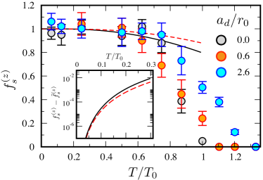
Figure 4: Superfluid fraction $f_{s}^{(z)}$ as a function of the scaled temperature $T/T_{0}$ at $nr_{0}^{3}=10^{-2}$ for three values of the dipolar lengths: a) SF with $a_{d}=0$ (hard-core bosons), b) SF with $a_{d}=0.6r_{0}$, c) FP with $a_{d}=2.6\,r_{0}$. Lines refer to the analytical prediction of the temperature dependence of the superfluid fraction at $nr_{0}^{3}=10^{-2}$ from Eq.(3) at $a_{d}=0$ (black continuous line) and $a_{d}=0.6\,r_{0}$ (red dashed line). Inset. Low temperature limit of $f_{s}^{(z)}$ from Eq.(3) and Eq.(5) in the SF at $a_{d}=0$ and $a_{d}=0.6\,r_{0}$.

Our results then suggest that the observed interference pattern kadau2016 is a consequence of local phase coherence (within each droplet) and not a global one. As discussed above the FP is characterized by an anisotropic superfluid density that, interestingly, might be measured via the second sound along the orthogonal directions as done with strongly interacting Fermi gases verney2015 ; tey2013 ; pitaevskii2015 ; hou2013 .

In this Letter we studied the many-body phases of an ensemble of bosons interacting via dipole-dipole interactions in three dimensional free space and investigated the superfluid behavior of dipolar filaments. We spanned a wide range of the parameter space confirming the existence of an extended phase of filaments with unitary superfluidity along the vertical direction and vanishing otherwise. Our results therefore theoretically support recent experimental findings about the stability of droplets in free space schmitt2016 and the presence of local phase coherence kadau2016 giving rise to interference fringes but exclude global phase coherence of the filaments nota3 and therefore a possible supersolid phase. Finally we confirmed that filaments are stable at finite temperature. More refined investigations are needed to determine accurately the melting transition of the filaments into a fluid phase.

Supplemental Materials: Superfluid filaments of dipolar bosons

.1 Density profile in the Filament Phase

In Fig.S1 we analyze the density on few filaments in the FP at $n\,r_{0}^{3}=10^{-2}$. We fit the density with a gaussian and extract the average number of particles within each filament. The inset shows the width of the gaussian in units of $r_{0}$ as a function of the particle number. The estimate of the average inter-particle distance with a gaussian wave packet in the radial direction and a cylinder of length $L$ along $z$ gives

$$\left<r\right>\approx\frac{1}{n^{1/3}}=\left(\frac{\pi a_{\perp}^{2}L}{N}\right)^{1/3}=2.1\,r_{0}$$ (S1)

for the data of Fig.S1 below. This result is also in agreement with the calculation of the radial correlation function $g_{\perp}(r)$ of Fig.2b (bottom) which is peaked at $r\approx 2r_{0}$.

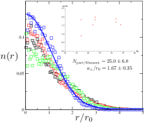
Figure S1: Particle density within a filament as a function of $r/r_{0}$. For this filament the average particle number is $N=25$.

.2 Relation among scattering length, dipolar length and cutoff radius and universality

The relation between the dipolar length and the scattering length for the potential of Eq.(2) of the text is discussed in detail in bortolotti2006 ; ronen2006 . In Fig.S2 below we show the relation between $a_{s}$ and $a_{d}$ in units of $r_{0}$. At $a_{d}/r_{0}\approx 2.9$ and $a_{d}/r_{0}\approx 6.5$ there are resonances at which the scattering length $a_{s}$ diverges. From Fig.S2 one can extract the value of $\epsilon_{d}=a_{d}/a_{s}$ as a function of the corresponding ratios $a_{s}/r_{0}$ and $a_{d}/r_{0}$ (see below Fig.S3).

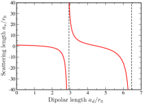
Figure S2: Relation between scattering length $a_{s}$ and dipolar length $a_{d}$ in units of $r_{0}$. Data are taken from ronen2006 .

.2.1 Universality of the results of the phase diagram obtained with the model potential

The cutoff radius $r_{0}$ of the model potential in Eq.2 in the main text is used to enable simulations within our QMC numerical scheme. In bortolotti2006 ; ronen2006 the authors numerically compute the full low-energy scattering amplitude for the same model potential and compare it with the one obtained from the first Born approximation within the pseudo-potential of Yi and Yu yi2000 ; yi2001

$$V_{\text{eff}}(\mathbf{r})=\frac{4\pi\hbar^{2}a_{s}(a_{d})}{m}\delta(\mathbf{r})+\frac{C_{dd}}{4\pi}\frac{1-3\cos^{2}\theta}{r^{3}}.$$ (S2)

Upon varying the ratio $a_{d}/r_{0}$ they find a remarkably good matching of the scattering amplitudes obtained with the two approaches in the very low energy limit, once including an explicit dependence of the scattering length $a_{s}(a_{d})$ on the dipolar length $a_{d}$. In this respect the results obtained in our phase diagram lie in the universal regime, since only $a_{s}$ and $a_{d}$ are relevant parameters.

It is worth mentioning that more realistic model potentials (with Van der Walls short range potentials) were recently considered in jachymski2016 for the description of Dysprosium two-body collisions. These potentials eventually lead to the same effective potential of Yi and Yu above, with a dipolar length depending on the short range scattering length.

.3 Phase diagram and comparison with experimental parameters of ¹⁶²Dy and ¹⁶⁴Dy

We compare our theoretical results with recent experiments with ¹⁶²Dy and ¹⁶⁴Dy which have dipolar lengths $a_{d}=129.2\,a_{0}$ and $130.8\,a_{0}$ respectively. As an example we analyze the case of fixed average density $n=5\cdot 10^{20}$ m^-3 and derive the blue curve in our phase diagram corresponding to this condition. Namely from $n\,a_{d}^{3}=2\cdot 10^{-4}$, we write:

$$n\,r_{0}^{3}=\frac{n\,a_{d}^{3}}{\left(a_{d}/r_{0}\right)^{3}}.$$ (S3)

(For simplicity we fix $a_{d}=130\,a_{0}$ for both components since the deviation is not significant). The background scattering length were recently measured for both isotopes tang2016 ; maier2015 ; burdick2016 :

$${}^{162}\text{Dy}=122\,a_{0}\ \ \ \ ^{164}\text{Dy}=92\,a_{0}.$$ (S4)

Using the parametrization of Fig.S2 we are able to identify the two points in the phase diagram. Notice that the experimental results lie in the transition region (within the error bars) from SF to CP. In the lower part of the figure we zoom on the relevant part of the phase diagram and compute $\epsilon_{d}=a_{d}/a_{s}$ and the parameter $n\,a_{s}^{3}$. From the calculation of $\epsilon_{d}$ for the two isotopes we can also compute the value of the parameter $r_{0}$:

$${}^{162}\text{Dy:}\ r_{0}=177\,a_{0}\ \ \ ^{164}\text{Dy:}\ r_{0}=154\,a_{0}.$$ (S5)

In Fig.S4-a we show a configuration in the cluster phase for $a_{d}=1.25\,r_{0}$ corresponding to $\epsilon=4.5$ ($a_{s}=29\,a_{0}$) at $n\,r_{0}^{3}=10^{-4}$ along the same blue line of the experimental data. In the right panel Fig.S4-b we plot the permutation cycles for the same parameters, showing permutations within the cluster, supporting the interpretation that locally particles exchange and quantum droplets are locally superfluid.

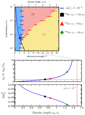
Figure S3: ¹⁶²Dy and ¹⁶⁴Dy phase line for $n\cdot a_{d}^{3}=2\cdot 10^{-4}$. (Top) Upon fixing the average density to $n=5\cdot 10^{20}$ m^-3 and the dipolar length to $a_{d}=130\,a_{0}$ we find that the condition $n\cdot a_{d}^{3}=2\cdot 10^{-4}$ is parametrized by the solid blue line in the phase diagram above. (Bottom) Ratio $\epsilon_{d}$ between the dipolar length $a_{d}$ and the scattering length $a_{s}$ computed from Fig.S2 above. Below we plot the parameter $n\,a_{s}^{3}$ along the blue line in the phase diagram. The red dashed line represents the line for which the scattering length as vanishes. Black square and red triangle correspond to experimental parameters for Dy with their background scattering length ($122\,a_{0}$ and $92\,a_{0}$ respectively). Green diamond is the point for Dy with $a_{s}=29\,a_{0}$ for which $n\,r_{0}^{3}=10^{-4}$ in the CP.

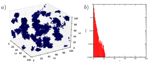
Figure S4: a) Configuration in the cluster phase for $a_{d}/r_{0}=1.2$ and $n\,r_{0}^{3}=10^{-4}$. The simulation is done along the blue curve in the phase diagram. b) Permutation cycles for the same parameters in fig.a).

.4 Weakly interacting regime

Figure S5: Universality of the model potential used in simulations. In the interval used in the simulations we plot the curves corresponding to $n\,\left|a_{s}\right|^{3}=5\cdot 10^{-3}$ (dashed) and $n\,a_{d}^{3}=5\cdot 10^{-3}$ (solid). The blue region displays the parameter space where both the inequalities $n\,\left|a_{s}\right|^{3}\leq 5\cdot 10^{-3}$ and $n\,a_{d}^{3}\leq 5\cdot 10^{-3}$ are satisfied. The red dashed line shows the position of the resonance where divergence of the scattering length diverges. The red diamond at $n\,r_{0}^{3}=10^{-3}$ and the orange square at $n\,r_{0}^{3}=10^{-4}$ and $a_{d}/r_{0}=3$ correspond to configurations of Fig. S5.

In our phase diagram we vary $n\,r_{0}^{3}$ in the range $6\cdot 10^{-5}-10^{-1}$. To answer the question whether the many-body physics of our model could be described by a universal weakly interacting theory, we compute $n\,\left|a_{s}\right|^{3}$ and $n\,a_{d}^{3}$ and verify whether the conditions:

$$n\,\left|a_{s}\right|^{3}\ll 1,\ \ \ \ \ n\,a_{d}^{3}\ll 1$$ (S6)

are simultaneously satisfied. In other words, both potential length scales are much smaller than the inter-particle distance. In Fig.S5 we plot the curves corresponding to $n\,\left|a_{s}\right|^{3}=5\cdot 10^{-3}$ (dashed lines) and $n\,a_{d}^{3}=5\cdot 10^{-3}$ (solid lines). The shaded region depicts the region where both inequalities:

$$n\,\left|a_{s}\right|^{3}\leq 5\cdot 10^{-3},\ \ \ \ \ n\,a_{d}^{3}\leq 5\cdot 10^{-3}$$ (S7)

hold. Note that the weakly interacting regime is the one for small values of the ratio $a_{d}/r_{0}$, and that the presence of a resonance at $a_{d}/r_{0}\approx 2.9$ introduces a small region where the inequalities (S7) are both satisfied. In Fig.S5 we show two snapshots of QMC configurations close to resonance at $a_{d}/r_{0}=3$ for $n\,r_{0}^{3}=10^{-4}$ and $n\,r_{0}^{3}=10^{-3}$ respectively. In both cases $\epsilon=0.12$, and a mean field theory would predict a superfluid phase. However as we commented above, this is not necessarily true, since in both cases we are outside the weakly interacting regime. Indeed both configurations clearly show that the system is in a cluster phase for such parameters.

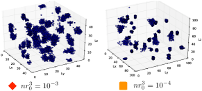
Figure S6: Snapshots of configurations for $N=100$ particles at $a_{d}/r_{0}=3$. (Left) $n\,r_{0}^{3}=10^{-4}$, (right) $n\,r_{0}^{3}=10^{-3}$. For both the scattering length equals $a_{s}/r_{0}=26$, therefore $\epsilon=0.12$. Both configurations refer to the points in Fig.S4. The system is in the cluster phase and not in a superfluid one contrarily to what is predicted by mean field theory.

.5 Radial distribution function

In Fig.2 of the main text we plot the radial distribution function along the vertical direction $g_{\parallel}(r)$ and along the plane $g_{\perp}(r)$ properly averaged as follows. To compute $g_{\parallel}(r)$ we first divide the plane $x-y$ into small squares and then compute the radial distribution function following the standard definition (see chaikin1995 ) properly normalized along a parallelepiped with height given by half the length of the box edge. Finally we average the resulting function over all the squares in the plane and all the slices of each configuration. We repeat this process for $100$ configurations to obtain the curves of Fig.2. We proceed analogously for $g_{\perp}(r)$ where the radial distribution function is computed along along a parallelepiped with the horizontal basis coinciding with the basis of the simulation box.

References

- (1) D. C. E. Bortolotti, S. Ronen, J. L. Bohn, and D. Blume, Phys. Rev. Lett. 97, 160402 (2006).
- (2) S. Ronen, D. C. E. Bortolotti, D. Blume, and J. L. Bohn, Phys. Rev. A 74, 033611 (2006).
- (3) S. Yi and L. You, Phys. Rev. A 61, 041604(R) (2000).
- (4) S. Yi and L. You, Phys. Rev. A 63, 053607 (2001).
- (5) R. Oldziejewski and K. Jachymski, Phys. Rev. A 94, 063638 (2016).
- (6) Y. Tang, A. Sykes, N.Q. Burdick, J.L. Bohn, and B.L. Lev, Phys. Rev. A. 92, 022703 (2016).
- (7) T. Maier, I. Ferrier-Barbut, H. Kadau, M. Schmitt, M. Wenzel, C. Wink, T. Pfau, K. Jachymski, and P. S. Julienne, Phys. Rev. A 92, 060702(R) (2015)
- (8) N.Q Burdick,, A. Sykes, Y. Tang and B.L Lev, New J. Phys. 18, 113004 (2016).
- (9) P. M. Chaikin and T. C. Lubensky, Principles of Condensed Matter (Ed. Cambridge University Press 1995).