Characterizing variability in nonlinear,
recurrent neuronal networks

Abstract

In this note, we develop semi-analytical techniques to obtain the full correlational structure of a stochastic network of nonlinear neurons described by rate variables. Under the assumption that pairs of membrane potentials are jointly Gaussian – which they tend to be in large networks – we obtain deterministic equations for the temporal evolution of the mean firing rates and the noise covariance matrix that can be solved straightforwardly given the network connectivity. We also obtain spike count statistics such as Fano factors and pairwise correlations, assuming doubly-stochastic action potential firing. Importantly, our theory does not require fluctuations to be small, and works for several biologically motivated, convex single-neuron nonlinearities.

1 Introduction

In this technical note, we develop a novel theoretical framework for characterising across-trial (and temporal) variability in stochastic, nonlinear recurrent neuronal networks with rate-based dynamics. We consider networks in which momentary firing rates $\mathbf{r}$ are given by a nonlinear function of the underlying (coarse-grained) membrane potentials $\mathbf{u}$. In particular, we treat the case of the threshold-power-law nonlinearity $r=k\lfloor u\rfloor_{+}^{n}$ (where $n$ is an arbitrary positive integer), which has been shown to approximate the input-output function of real cortical neurons (with $n$ ranging from 1 to 5; Priebe et al.,, 2004; Miller and Troyer,, 2002). This model is of particular interest as it captures many of the nonlinearities observed in the trial-averaged responses of primary visual cortex (V1) neurons to visual stimuli (Ahmadian et al.,, 2013; Rubin et al.,, 2015), as well as the stimulus-induced suppression of (co-)variability observed in many cortical areas (Hennequin et al.,, submitted).

We derive assumed density filtering equations that describe the temporal evolution of the first two moments of the joint probability distribution of membrane potentials and firing rates in the network. These equations are based on the assumption that pairs of membrane potentials are jointly Gaussian at all times, which tends to hold in large networks. This approach allows us to solve the temporal evolution of the mean firing rates and the across-trial noise covariance matrix, given the model parameters (network connectivity, feedforward input to the network, and statistics of the input noise). We also obtain the full firing rate cross-correlogram for any pair of neurons, which allows us to compute both Fano factors and pairwise spike count correlations in arbitrary time windows, assuming doubly stochastic (inhomogeneous Poisson) spike emission. Importantly, our theory does not require fluctuations to be small, and is therefore applicable to physiologically relevant regimes where spike count variability is well above Poisson variability (implying large fluctuations of $\mathbf{u}$, which is therefore often found below the threshold of the nonlinearity).

This note is structured as follows. We first provide all the derivations, together with a summary of equations and some practical details on implementation. We then demonstrate the accuracy of our approach on two different networks of excitatory and inhibitory neurons: a random, weakly connected network, and a random, strongly connected but inhibition-stabilized network. In the latter case, the stochastic dynamics are dominated by balanced (nonnormal) amplification, leading to the emergence of strong correlations between neurons (Murphy and Miller,, 2009; Hennequin et al.,, 2014) which could in principle make the membrane potential distribution non-Gaussian – the only condition that could break the accuracy of our theory. Even in this regime, we obtain good estimates of the first and second-order moments of the joint distributions of both $\mathbf{u}$ and $\mathbf{r}$.

2 Theoretical results

Notations

We use $\cdot^{\mathop{\rm T}}$ to denote the vector/matrix transpose, bold letters to denote column vectors ($\mathbf{v}\equiv(v_{1},\ldots,v_{N})^{\mathop{\rm T}}$) and bold capitals for matrices (e.g. $\mathbf{W}=\{W_{ij}\}$) . The notation $\text{diag}(\mathbf{v})$ is used for the diagonal matrix with entries $v_{1},v_{2},\ldots,v_{N}$ along the diagonal.

2.1 Model setup

We consider a network of $N$ interconnected neurons, whose continuous-time, stochastic and nonlinear dynamics follow

$$\mathrm{d}u_{i}\quad=\quad\frac{\mathrm{d}t}{\tau_{i}}\left(-u_{i}(t)+h_{i}(t)+\sum_{j}W_{ij}\>r_{j}(t)\right)+\mathrm{d}\chi_{i}$$ (1)

where the momentary firing rate $r_{j}(t)$ is given by a positive, nonlinear function $f$ of $u_{j}(t)$:

$$r_{j}(t)=f\left[u_{j}(t)\right]$$ (2)

The first few derivations below hold for arbitrary nonlinearity $f$; we will commit to the threshold-powerlaw nonlinearity $f(u)\propto\lfloor u\rfloor_{+}^{n}$ only later. In Equation 1, $\tau_{i}$ is the intrinsic (“membrane”) time constant of unit $i$, $h_{i}(t)$ denotes a deterministic and perhaps time-varying feedforward input, $W_{i\ell}$ is the synaptic weight from unit $\ell$ onto unit $i$, and $\mathrm{d}\bm{\chi}$ is a multivariate Wiener process with covariance $\langle\chi_{i}(t)\>\chi_{j}(t+s)\rangle=\Sigma^{\chi}_{ij}\delta(s)$. Note that the elements of $\mathbf{\Sigma}^{\chi}$ have units of $({\rm mV})^{2}/s$. We will later extend Equation 1 to the case of temporally correlated input noise.

Most of our results can be derived from the finite-difference version of Equation 1, given for very small $\epsilon$ by

$$u_{i}(t)-u_{i}(t-\epsilon)\quad=\quad\frac{\epsilon}{\tau_{i}}\left[-u_{i}(t-\epsilon)+h_{i}(t)+\sum_{\ell}W_{i\ell}\>r_{\ell}(t-\epsilon)\right]+\sqrt{\epsilon}\>\chi_{i}(t)$$ (3)

Here $\bm{\chi}(t)$ is drawn from a multivariate normal distribution with covariance matrix $\mathbf{\Sigma}^{\chi}$, independently of the state of the sytem in the previous time step ($t-\epsilon$).

We now show how to derive deterministic equations of motion for the first and second-order moments of $\mathbf{u}$, then explain how these can be made self-consistent using the Gaussian assumption mentioned in the introduction. Solving these equations is straightforward, and returns the mean membrane potential of each neuron as well as the full matrix of pairwise covariances. We also show how the moments of $\mathbf{r}$ can be derived from those of $\mathbf{u}$, and how Fano factors and spike count correlations can then be obtained from those.

2.2 Temporal evolution of the moments of the voltage

We are interested in the moments of the membrane potential variables, defined as

$$\mu_{i}(t)\quad \equiv\quad\langle u_{i}(t)\rangle$$ (4a)

$$\Sigma_{ij}(t,s)\quad \equiv\quad\langle\tilde{u}_{i}(t)\>\tilde{u}_{j}(t+s)\rangle$$ (4b)

where $\langle\cdot(t)\rangle$ denotes ensemble averaging (or “trial-averaging”, i.e. an average over all possible realisations of the noise processes $\bm{\chi}(t^{\prime})$ for $0\leq t^{\prime}\leq t$), and with the notation $\tilde{z}(t)\equiv z(t)-\langle z(t)\rangle$. Note that $\langle\cdot(t)\rangle$ will coincide with temporal averages in the stationary case when the dynamics has a single fixed point (ergodicity). Before we proceed, let us introduce similar notations for other moments:

$$\nu_{i}(t)\quad \equiv\quad\langle r_{i}(t)\rangle$$ (5a)

$$\Gamma_{ij}(t,s)\quad \equiv\quad\langle\tilde{u}_{i}(t)\>\tilde{r}_{j}(t+s)\rangle$$ (5b)

$$\Lambda_{ij}(t,s)\quad \equiv\quad\langle\tilde{r}_{i}(t)\>\tilde{r}_{j}(t+s)\rangle$$ (5c)

Taking the ensemble average of Equation 3 and the limit $\epsilon\to 0$ yields a differential equation for the membrane potential mean:

$$\tau_{i}\>\frac{\mathrm{d}\mu_{i}}{\mathrm{d}t}=-\mu_{i}(t)+h_{i}(t)+\sum_{j}W_{ij}\>\nu_{j}(t)$$ (6)

We now subtract its average from Equation 3:

$$\tilde{u}_{i}(t)-\tilde{u}_{i}(t-\epsilon)=\frac{\epsilon}{\tau_{i}}\left[-\tilde{u}_{i}(t-\epsilon)+\sum_{j}W_{ij}\>\tilde{r}_{j}(t-\epsilon)\right]+\sqrt{\epsilon}\>\chi_{i}(t)$$ (7)

The equations of motion for the variances and covariances can be obtained in a number of ways. Here we adopt a simple approach based on the finite differences of Equation 7, observing that

$$\tilde{u}_{i}(t)\>\tilde{u}_{j}(t)-\tilde{u}_{i}(t-\epsilon)\>\tilde{u}_{j}(t-\epsilon)=\tilde{u}_{i}(t)\>\left[\tilde{u}_{j}(t)-\tilde{u}_{j}(t-\epsilon)\right]+\tilde{u}_{j}(t-\epsilon)\left[\tilde{u}_{i}(t)-\tilde{u}_{i}(t-\epsilon)\right]$$ (8)

Substituting Equation 7 into Equation 8, we obtain

$$\tilde{u}_{i}(t)\>\tilde{u}_{j}(t)-\tilde{u}_{i}(t-\epsilon)\>\tilde{u}_{j}(t-\epsilon)= -\frac{\epsilon}{\tau_{i}}\>\tilde{u}_{i}(t-\epsilon)\>\tilde{u}_{j}(t-\epsilon)-\frac{\epsilon}{\tau_{j}}\>\tilde{u}_{i}(t)\>\tilde{u}_{j}(t-\epsilon)$$ (9)

$$+\epsilon\sum_{\ell}\tilde{r}_{\ell}(t-\epsilon)\left(\frac{W_{i\ell}}{\tau_{i}}\>\tilde{u}_{j}(t-\epsilon)+\frac{W_{j\ell}}{\tau_{j}}\>\tilde{u}_{i}(t)\right)$$

$$+\sqrt{\epsilon}\left(\chi_{i}(t)\>\tilde{u}_{j}(t)+\chi_{j}(t)\>\tilde{u}_{i}(t-\epsilon)\right)$$

We now take ensemble expectations on both sides. The l.h.s. of Equation 9 averages to $\Sigma_{ij}(t)-\Sigma_{ij}(t-\epsilon)$. The term $\chi_{j}(t)\>\tilde{u}_{i}(t-\epsilon)$ averages to zero for any $(i,j)$ pair, because the input noise terms at time $t$ are independent of the state of the system at time $t-\epsilon$. However, we expect the equal-time product $\chi_{i}(t)\>\tilde{u}_{j}(t)$ to average to something small ($\mathcal{O}(\sqrt{\epsilon})$) but non-zero. Let us compute it, by recalling that

$$\tilde{u}_{j}(t)=\tilde{u}_{j}(t-\epsilon)+\frac{\epsilon}{\tau_{j}}\left[\>\text{something at time}\>(t-\epsilon)\>\right]+\sqrt{\epsilon}\>\chi_{j}(t)$$ (10)

Multiplying both sides by $\chi_{i}(t)$ and taking expectations, again all products of $\chi_{i}(t)$ with quantities at time $t-\epsilon$ vanish, and we are left with

$$\langle\tilde{u}_{j}(t)\>\chi_{i}(t)\rangle\quad=\quad\Sigma^{\chi}_{ij}\sqrt{\epsilon}$$ (11)

Thus, when averaged, Equation 9 becomes

$$\frac{\Sigma_{ij}(t)-\Sigma_{ij}(t-\epsilon)}{\epsilon}=-\frac{\Sigma_{ij}(t-\epsilon,0)}{\tau_{i}}-\frac{\Sigma_{ij}(t,-\epsilon)}{\tau_{j}}+\sum_{\ell}\left(\frac{W_{i\ell}}{\tau_{i}}\Gamma_{j\ell}(t-\epsilon,0)+\frac{W_{j\ell}}{\tau_{j}}\Gamma_{i\ell}(t,-\epsilon)\right)+\Sigma_{ij}^{\chi}$$ (12)

Now taking the limit of $\epsilon\to 0$, and by continuity of both $\mathbf{u}$ and $\mathbf{r}$, we obtain the desired equation of motion of the zero-lag covariances:

$$\frac{\mathrm{d}\Sigma_{ij}(t,0)}{\mathrm{d}t}=\Sigma^{\chi}_{ij}+\frac{1}{\tau_{i}}\left(-\Sigma_{ij}(t,0)+\sum_{\ell}W_{i\ell}\>\Gamma_{j\ell}(t,0)\right)+\frac{1}{\tau_{j}}\left(-\Sigma_{ij}(t,0)+\sum_{\ell}W_{j\ell}\>\Gamma_{i\ell}(t,0)\right)$$ (13)

In the special case of constant input $h_{i}(t)$, the covariance matrix of the steady-state, stationary distribution of potentials satisfies Equation 13 with the l.h.s. set to zero. This system of equations can be seen as a nonlinear extension of the classical Lyapunov equation for the multivariate (linear) Ornstein-Uhlenbeck process (Gardiner,, 1985), in which $W_{i\ell}\>\Sigma_{j\ell}$ would replace $W_{i\ell}\>\Gamma_{j\ell}$ inside the sum. Such linear equations have been derived previously in the context of balanced networks of threshold binary units (Renart et al.,, 2010; Barrett,, 2012; Dahmen et al.,, 2016).

We can also obtain the lagged cross-covariances by integrating the following differential equation – obtained using similar methods as above – over $s>0$:

$$\frac{\mathrm{d}\Sigma_{ij}(t,s)}{\mathrm{d}s}=\frac{1}{\tau_{j}}\left(-\Sigma_{ij}(t,s)+\sum_{\ell}W_{j\ell}\>\Gamma_{i\ell}(t,s)\right)$$ (14)

Covariances for negative time lags are then obtained from those at positive lags, since:

$$\mathbf{\Sigma}(t,-s)=\mathbf{\Sigma}(t-s,s)^{\mathop{\rm T}}.$$ (15)

In the stationary case, we have simply $\mathbf{\Sigma}(\infty,-s)=\mathbf{\Sigma}(\infty,s)^{\mathop{\rm T}}$. Equation 14 can be integrated with initial condition $\mathbf{\Sigma}(t,0)$ which is itself obtained by integrating Equations 6 and 13.

2.3 Calculation of nonlinear moments

To be able to integrate Equations 6, 13 and 14, we need to express the nonlinear moments $\bm{\nu}$ and $\mathbf{\Gamma}$ as a function of $\bm{\mu}$ and $\mathbf{\Sigma}$. This is a moment closure problem, which in general cannot be solved exactly. Here, we will approximate $\bm{\nu}$ and $\mathbf{\Gamma}$ by making a Gaussian process assumption for $\mathbf{u}$: we assume that for any pair of neurons $(i,j)$ and any pair of time points $(t,t+s)$, the potentials $u_{i}(t)$ and $u_{j}(t+s)$ are jointly Gaussian, i.e.

$$\forall(i,j),\ \forall(t,s)\qquad\left(\begin{array}[]{c}u_{i}(t)\\ u_{j}(t+s)\end{array}\right)\sim\mathcal{N}\left[\left(\begin{array}[]{c}\mu_{i}(t)\\ \mu_{j}(t+s)\end{array}\right),\left(\begin{array}[]{lr}\Sigma_{ii}(t,0)&\Sigma_{ij}(t,s)\\ \Sigma_{ij}(t,s)&\Sigma_{jj}(t+s,0)\end{array}\right)\right]$$ (16)

In other words, we systematically and consistently ignore all moments of order 3 or higher. This is the strongest assumption we make here, but its validity can always be checked empirically by running stochastic simulations. For certain firing rate nonlinearities $f$ (in particular, threshold-power law functions), the Gaussian process assumption will enable a direct and exact calculation of $\bm{\nu}$ and $\mathbf{\Gamma}$ given $\bm{\mu}$ and $\mathbf{\Sigma}$, with no need to linearise the dynamics, as detailed below.

From now on, we will drop the time dependence from the notations to keep the derivations uncluttered, with the understanding that in using the results that follow to compute second-order moments such as $\Gamma_{ij}(t,s)$ or $\Lambda_{ij}(t,s)$, the quantities $\mu_{i}$ and variances $\Sigma_{ii}$ that regard neuron $i$ will have to be evaluated at time $t$, those that regard neuron $j$ evaluated at time $t+s$, and any covariance $\Sigma_{ij}$ will have to be understood as $\Sigma_{ij}(t,s)$ as defined in Equation 4b.

Using the Gaussian assumption, mean firing rates become Gaussian integrals:

$$\nu_{i}\quad=\quad\int\mathcal{D}z\cdot f\left(\mu_{i}+z\sqrt{\Sigma_{ii}}\right)$$ (17)

where $\mathcal{D}z$ denotes the standard Gaussian measure, and $f(\cdot)$ is the firing rate nonlinearity (cf. Equation 2). Similarly,

$$\Gamma_{ij}\quad=\quad\iint\mathrm{d}u_{i}\>\mathrm{d}u_{j}\cdot\mathcal{N}\left[\left(\begin{array}[]{c}u_{i}\\ u_{j}\end{array}\right);\left(\begin{array}[]{c}\mu_{i}\\ \mu_{j}\end{array}\right),\left(\begin{array}[]{cc}\Sigma_{ii}&\Sigma_{ij}\\ \Sigma_{ij}&\Sigma_{jj}\end{array}\right)\right]\cdot(u_{i}-\mu_{i})\cdot f(u_{j})$$ (18)

To calculate $\Gamma_{ij}$, we make use of the fact that the elliptical Gaussian distribution with correlation $c_{ij}=\Sigma_{ij}/\sqrt{\Sigma_{ii}\Sigma_{jj}}$ in Equation 18 can be turned into a spherical Gaussian via a change of variable:

$$\Gamma_{ij}=\iint\mathcal{D}z\>\mathcal{D}z^{\prime}\cdot\sqrt{\Sigma_{ii}}\left(z^{\prime}c_{ij}+z\sqrt{1-c_{ij}^{2}}\right)\cdot f\left(\mu_{j}+z^{\prime}\sqrt{\Sigma_{jj}}\right)$$ (19)

Now, the integral over $z$ can be performed inside the other one, and clearly vanishes. We are left with

$$\Gamma_{ij}=c_{ij}\sqrt{\Sigma_{ii}}\int\mathcal{D}u\cdot u\cdot f\left(\mu_{j}+u\sqrt{\Sigma_{jj}}\right)$$ (20)

Finally, integrating by part (assuming the relevant integrals exist), we obtain a simpler form:

$$\Gamma_{ij}=\Sigma_{ij}\gamma_{j}$$ (21)

with

$$\gamma_{j}\equiv\int\mathcal{D}u\cdot f^{\prime}\left(\mu_{j}+u\sqrt{\Sigma_{jj}}\right)$$ (22)

The one-dimensional integrals in Equations 17 and 22 turn out to have closed-form solutions for a number of nonlinearities $u\mapsto f(u)$, including the exponential $f(u)\propto\exp(u)$ (Buesing et al.,, 2012) and the class of threshold power-law nonlinearities of the form $f(u)=k\lfloor u\rfloor_{+}^{n}$ for any integer exponent $n\geq 1$, which closely match the behavior of real cortical neurons under realistic noise conditions (Priebe et al.,, 2004; Miller and Troyer,, 2002).

In the threshold-powerlaw case $r=k\lfloor u\rfloor_{+}^{n}$, integration by parts yields the following recursive formulas:

$$\nu_{i}^{(n)} =\begin{cases}\displaystyle k\mu_{i}\>\psi\left(\frac{\mu_{i}}{\sqrt{\Sigma_{ii}}}\right)+k\sqrt{\Sigma_{ii}}\>\phi\left(\frac{\mu_{i}}{\sqrt{\Sigma_{ii}}}\right)&{\rm if}\ n=1\\ \displaystyle\mu_{i}\nu_{i}^{(1)}+k\Sigma_{ii}\psi\left(\frac{\mu_{i}}{\sqrt{\Sigma_{ii}}}\right)&{\rm if}\ n=2\\ \displaystyle\mu_{i}\>\nu_{i}^{(n-1)}+(n-1)\Sigma_{ii}\nu_{i}^{(n-2)}&{\rm otherwise}\end{cases}$$ (23)

$$\gamma_{i}^{(n)} =\begin{cases}\displaystyle k\psi\left(\frac{\mu_{i}}{\sqrt{\Sigma_{ii}}}\right)&{\rm if}\ n=1\\ \displaystyle n\>\nu_{i}^{(n-1)}&{\rm otherwise}\end{cases}$$ (24)

where $\phi$ and $\psi$ denote the standard Gaussian probability density function and its cumulative density function respectively.

Plugging the moment-conversion results of Equations 23 and 24 into the equations of motion (Equations 6, 13 and 14) yields a system of self-consistent, deterministic differential equations for the temporal evolution of the potential distribution (or its moments). These equations can be integrated straightforwardly given the initial moments at time $t=0$.

If we are interested in the stationary distribution of $\mathbf{u}(t)$ or $\mathbf{r}(t)$, i.e. in the case where $h_{i}(t)=\mathrm{constant}$, we can start from any valid initial condition $(\bm{\mu},\mathbf{\Sigma})$ with $\mathbf{\Sigma}\succ 0$, and let the integration of Equations 6 and 13 converge to a fixed point. In the ergodic case, this will indeed converge to a unique stationary distribution, independent of the initial conditions used to integrate the equations of motion. If there are several fixed points, this procedure yields the moments of the stationary distribution of $\mathbf{u}$ conditioned on the initial conditions, i.e. will discover only one of the fixed points and return the moments of the fluctuations around it. Our approach cannot capture multistability explicitly, that is, it ignores the possibility that the network could change its set point with non-zero probability.

Finally, let us emphasise that we have never required that fluctuations be small. As long as the Gaussian assumption holds for the membrane potentials (Equation 16), we expect to obtain accurate solutions which is confirmed below in our numerical examples. This is because we have been able to express the moments of $\mathbf{r}$ as a function of those of $\mathbf{u}$ in closed form, without approximation.

2.4 Extension to temporally correlated input noise

So far, we have considered spatially correlated, but temporally white, external noise sources. We now extend our equations to the case of noise with spatiotemporal correlations, assuming space and time are separable, and temporal correlations in the input fall off exponentially with time constant $\tau_{\eta}$:

$$\tau_{i}\>\frac{\mathrm{d}u_{i}}{\mathrm{d}t}=-u_{i}(t)+h_{i}(t)+\sum_{\ell}W_{i\ell}\>r_{\ell}(t)+\eta_{i}(t)$$ (25)

with $\langle\eta_{i}(t)\rangle=0$ and $\langle\eta_{i}(t)\>\eta_{j}(t+s)\rangle\equiv\Sigma_{ij}^{\eta}e^{-|s|/\tau_{\eta}}$. The equation for the mean voltages (Equation 6) does not change. For the voltage covariances, however, Equation 13 becomes

$$\frac{\mathrm{d}\Sigma_{ij}(t,0)}{\mathrm{d}t}\quad =\quad\frac{1}{\tau_{i}}\left(-\Sigma_{ij}(t,0)+\sum_{\ell}W_{i\ell}\>\Gamma_{j\ell}(t,0)+\Sigma^{\star}_{ij}(t)\right)$$

$$+\quad\frac{1}{\tau_{j}}\left(-\Sigma_{ij}(t,0)+\sum_{\ell}W_{j\ell}\>\Gamma_{i\ell}(t,0)+\Sigma^{\star}_{ji}(t)\right)$$ (26)

with the definition $\Sigma^{\star}_{ij}(t)\equiv\langle\eta_{i}(t)\>\tilde{u}_{j}(t)\rangle$. These moments can also be obtained by simultaneously integrating the following:

$$\frac{\mathrm{d}\Sigma^{\star}_{ij}(t)}{\mathrm{d}t}\quad =\quad-\frac{\Sigma^{\star}_{ij}(t)}{\tau_{\eta}}+\frac{1}{\tau_{j}}\left(-\Sigma^{\star}_{ij}(t)+\Sigma_{ij}^{\eta}+\sum_{\ell}W_{j\ell}\>\Gamma^{\star}_{i\ell}(t)\right)$$ (27)

with an analogous definition $\Gamma^{\star}_{ij}(t)\equiv\langle\eta_{i}(t)\>\tilde{r}_{j}(t)\rangle=\Sigma_{ij}^{\star}(t)\gamma_{j}(t)$, which can be expressed self-consistently as a function of $\mu_{j}(t)$, $\Sigma_{jj}(t)$, and $\Sigma^{\star}_{ij}(t)$ according to Equations 21 and 24. Altogether, Equations 6, 2.4 and 27 form a set of closed and coupled differential equations for $\{\mu_{i}(t)\}_{i}$ and $\{\Sigma_{ij}(t,0)\}_{i\geq j}$ which can be integrated straightforwardly.

Temporal correlations are given by (for $s>0$):

$$\frac{\mathrm{d}\Sigma_{ij}(t,s)}{\mathrm{d}s}\quad=\quad\frac{1}{\tau_{j}}\left[-\Sigma_{ij}(t,s)+\sum_{\ell}W_{j\ell}\>\Gamma_{i\ell}(t,s)+\Sigma^{\star}_{ji}(t)\>\exp\left(-\frac{s}{\tau_{\eta}}\right)\right]$$ (28)

2.5 Summary of equations

The equations of motion for the moments of $\mathbf{u}$ can be summarised in matrix form as follows.

Temporally white input noise
Dynamics $\displaystyle\mathrm{d}\mathbf{u}\quad$ $\displaystyle=\quad\mathbf{T}^{-1}\left[-\mathbf{u}(t)+\mathbf{h}(t)+\mathbf{W}\mathbf{r}(t)\right]\mathrm{d}t+d\bm{\chi}$ (29) Mean $\displaystyle\frac{\mathrm{d}\bm{\mu}(t)}{\mathrm{d}t}\quad$ $\displaystyle=\quad\mathbf{T}^{-1}\left[-\bm{\mu}(t)+\mathbf{h}(t)+\mathbf{W}\bm{\nu}(t)\right]$ (30) Covariance $\displaystyle\frac{\mathrm{d}\mathbf{\Sigma}(t,0)}{\mathrm{d}t}\quad$ $\displaystyle=\quad\mathbf{\Sigma}^{\chi}+\bm{\mathcal{J}}(t)\mathbf{\Sigma}(t,0)+\mathbf{\Sigma}(t,0)\bm{\mathcal{J}}(t)^{\mathop{\rm T}}$ (31) Lagged cov. $\displaystyle\frac{\mathrm{d}\mathbf{\Sigma}(t,s)}{\mathrm{d}s}\quad$ $\displaystyle=\quad\mathbf{\Sigma}(t,s)\bm{\mathcal{J}}(t+s)^{\mathop{\rm T}}$ (32) where we have defined $\mathbf{T}=\text{diag}(\tau_{1},\ldots,\tau_{N})$, and $\bm{\mathcal{J}}(t)\equiv\mathbf{T}^{-1}\left[\mathbf{W}\text{diag}(\gamma_{1}(t),\ldots,\gamma_{N}(t))-\mathbf{I}\right]$. In these equations, $\bm{\nu}(t)$ and $\bm{\gamma}(t)$ are given in closed form as functions of $\bm{\mu}(t)$ and $\mathbf{\Sigma}(t,0)$ according to Equations 23 and 24.

Temporally correlated input noise
Dynamics $\displaystyle\frac{\mathrm{d}\mathbf{u}}{\mathrm{d}t}\quad$ $\displaystyle=\quad\mathbf{T}^{-1}\left[-\mathbf{u}(t)+\mathbf{h}(t)+\mathbf{W}\mathbf{r}(t)+\bm{\eta}(t)\right]$ (33) Mean $\displaystyle\frac{\mathrm{d}\bm{\mu}(t)}{\mathrm{d}t}\quad$ $\displaystyle=\quad\mathbf{T}^{-1}\left[-\bm{\mu}(t)+\mathbf{h}(t)+\mathbf{W}\bm{\nu}(t)\right]$ (34) Covariance $\displaystyle\frac{\mathrm{d}\mathbf{\Sigma}(t,0)}{\mathrm{d}t}\quad$ $\displaystyle=\quad\left[\mathbf{T}^{-1}\mathbf{\Sigma}^{\star}(t)\right]+\left[\mathbf{T}^{-1}\mathbf{\Sigma}^{\star}(t)\right]^{\mathop{\rm T}}+\bm{\mathcal{J}}(t)\mathbf{\Sigma}(t,0)+\mathbf{\Sigma}(t,0)\bm{\mathcal{J}}(t)^{\mathop{\rm T}}$ (35) $\displaystyle\frac{\mathrm{d}\mathbf{\Sigma}^{\star}(t)}{\mathrm{d}t}\quad$ $\displaystyle=\quad-\frac{1}{\tau_{\eta}}\mathbf{\Sigma}^{\star}(t)+\mathbf{\Sigma}^{\eta}\mathbf{T}^{-1}+\mathbf{\Sigma}^{\star}(t)\bm{\mathcal{J}}(t)^{\mathop{\rm T}}$ (36) Lagged cov. $\displaystyle\frac{\mathrm{d}\mathbf{\Sigma}(t,s)}{\mathrm{d}s}\quad$ $\displaystyle=\quad e^{-s/\tau_{\eta}}\left[\mathbf{T}^{-1}\mathbf{\Sigma}^{\star}(t)\right]^{\mathop{\rm T}}+\mathbf{\Sigma}(t,s)\bm{\mathcal{J}}(t+s)^{\mathop{\rm T}}$ (37) with the same definitions of $\mathbf{T}$ and $\bm{\mathcal{J}}(t)$ as above, and with $\bm{\nu}(t)$ and $\bm{\gamma}(t)$ again given by Equations 23 and 24 as functions of $\bm{\mu}(t)$ and $\bm{\Sigma}(t,0)$.

Note on implementation

We favor using the equations of motion in their matrix form, as we can then use highly efficient libraries for vectorised operations, especially matrix products (we use the OpenBLAS library). We integrate Equations 30, 31 and 32 and Equations 34, 35, 36 and 37 using the classical Euler method with a small time step $\delta_{t}=0.1$ ms. When interested in the stationary moments, a good initial condition from which to start the integration is given by the case $\mathbf{W}=0$, i.e. $\bm{\mu}(0)\equiv\mathbf{h}$, $\mathbf{\Sigma}^{\star}(0)\equiv\mathbf{\Sigma}^{\eta}\text{diag}\left(\frac{1}{1+\bm{\tau}/\tau_{\eta}}\right)$, and $\mathbf{\Sigma}(0,0)$ obtained by solving a simple Lyapunov equation.

Care should be taken in integrating the covariance flow of Equations 31 and 35 to preserve the positive definiteness of $\mathbf{\Sigma}$ at all times. We do this for Equation 31 using the following integrator (Bonnabel and Sepulchre,, 2012):

$$\mathbf{\Sigma}(t+\delta_{t},0)=\left[\mathbf{I}+\delta_{t}\bm{\mathcal{J}}(t)\right]\mathbf{\Sigma}(t,0)\left[\mathbf{I}+\delta_{t}\bm{\mathcal{J}}(t)\right]^{\mathop{\rm T}}+\delta_{t}\mathbf{\Sigma}^{\chi}$$ (38)

and analogously for Equation 35. The complexity is $\mathcal{O}(TN^{3})$ where $T$ is the number of time bins, and $N$ is the number of neurons. In comparison, stochastic simulations of Equation 1 cost $\mathcal{O}(KTN^{2})$, where $K$ is a certain number of independent trials that must be simulated to get an estimate of activity variability. This complexity is only quadratic in $N$, but in practice $K$ will have to be large for the moments to be accurately estimated. Moreover, the generation of random numbers in Monte-Carlo simulations is expensive. In all the numerical examples given below, theoretical values were obtained at least 10 times faster than the corresponding Monte-Carlo estimates, given a decent accuracy criterion (required number of trials). Where appropriate, one could also apply low-rank reduction techniques to reduce the complexity of the equations of motion to $\mathcal{O}(TN^{2})$ (e.g. in the spirit of Bonnabel and Sepulchre,, 2012); this is left for future work.

2.6 Firing rate correlations

So far we have obtained results for pairwise membrane potential covariances $\Sigma_{ij}(t,s)$, but, as indicated above, these can also be translated into covariances between the corresponding rate variables, $\Lambda_{ij}(t,s)\equiv\left\langle\tilde{r}_{i}(t)\>\tilde{r}_{j}(t+s)\right\rangle$, which we will need later to compute spike count statistics (e.g. Fano factors or correlations). To shorten the notation, we again drop the time dependence, with the same understanding that in using the equations that follow to compute $\Lambda_{ij}(t,s)$, the quantities $\mu_{i}$ and variances $\Sigma_{ii}$ that regard neuron $i$ will have to be evaluated at time $t$, those that regard neuron $j$ evaluated at time $t+s$, and the covariance $\Sigma_{ij}$ will have to be understood as $\Sigma_{ij}(t,s)$.

Under the same Gaussian process assumption as above, we have

$$\Lambda_{ij}\quad=\quad\iint\mathrm{d}u\>\mathrm{d}u^{\prime}\cdot\mathcal{N}\left[\left(\begin{array}[]{c}u\\ u^{\prime}\end{array}\right);\left(\begin{array}[]{c}\mu_{i}\\ \mu_{j}\end{array}\right),\left(\begin{array}[]{cc}\Sigma_{ii}&\Sigma_{ij}\\ \Sigma_{ij}&\Sigma_{jj}\end{array}\right)\right]\cdot(f(u)-\nu_{i})\cdot(f(u^{\prime})-\nu_{j})$$ (39)

Calculating this double integral exactly seems infeasible. However, as detailed below, we were able to derive an analytical approximation that is highly accurate over a broad range of physiologically relevant values (Figure 1), for the class of threshold power-law nonlinearities $f(u)=k\lfloor u\rfloor_{+}^{n}$.

Numerical explorations of the behaviour of $\Lambda_{ij}$ as a function of the moments of $u_{i}$ and $u_{j}$ suggest the following ansatz:

$$\Lambda_{ij}\quad=\quad\alpha_{ij}^{(3)}c_{ij}^{3}+\alpha_{ij}^{(2)}c_{ij}^{2}+\alpha_{ij}^{(1)}c_{ij}$$ (40)

where $c_{ij}=\Sigma_{ij}/\sqrt{\Sigma_{ii}\Sigma_{jj}}$ is the correlation coefficient between $u_{i}$ and $u_{j}$ (at time $t$ and lag $s$), and the three coefficients $\alpha_{ij}^{(\cdot)}$ do not depend on $c_{ij}$ (though they depend on the marginals over $u_{i}$ and $u_{j}$, as detailed below) and can be computed exactly. We focus on $\Lambda_{ij}$ as a function of $c_{ij}$ – we abuse the notation of Equation 5c and write this dependence as $\Lambda_{ij}(c_{ij})$. Clearly, $\Lambda_{ij}(0)=0$. Next, we note that

$$\alpha_{ij}^{(2)}\quad =\quad\left[\Lambda_{ij}(+1)+\Lambda_{ij}(-1)\right]/2$$ (41a)

$$\alpha_{ij}^{(1)}+\alpha_{ij}^{(3)}\quad =\quad\left[\Lambda_{ij}(+1)-\Lambda_{ij}(-1)\right]/2$$ (41b)

$$\alpha_{ij}^{(1)}\quad =\quad\left.\frac{\mathrm{d}\Lambda_{ij}(c_{ij})}{\mathrm{d}c_{ij}}\right|_{c_{ij}=0}$$ (41c)

where, specialising to the threshold-power law nonlinearity $f(u)=k\lfloor u\rfloor_{+}^{n}$,

$$\Lambda_{ij}({\color[rgb]{1,0,0}{\pm}}1)\quad=\quad-\nu_{i}\>\nu_{j}+k^{2}\int\mathcal{D}u\ \lfloor\mu_{i}{\color[rgb]{1,0,0}\pm}u\sqrt{\Sigma_{ii}}\rfloor_{+}^{n}\ \lfloor\mu_{j}+u\sqrt{\Sigma_{jj}}\rfloor_{+}^{n}$$ (42)

After some algebra, Equation 41c yields

$$\alpha_{ij}^{(1)}=\left(\gamma_{i}\sqrt{\Sigma_{ii}}\right)\left(\gamma_{j}\sqrt{\Sigma_{jj}}\right)$$ (43)

where $\Gamma_{ii}$ and $\Gamma_{jj}$ were derived previously in Equations 21 and 24. To compute $\Lambda_{ij}(+1)$, let us define more generally

$$A_{ij}^{(n,m)}\equiv k^{2}\int\mathcal{D}u\ \lfloor\mu_{i}+u\sqrt{\Sigma_{ii}}\rfloor_{+}^{n}\ \lfloor\mu_{j}+u\sqrt{\Sigma_{jj}}\rfloor_{+}^{m}$$ (44)

keeping in mind that we are ultimately interested in $A_{ij}^{(n,n)}$, since $\Lambda_{ij}(+1)=-\nu_{i}\nu_{j}+A_{ij}^{(n,n)}$. In the following, we assume that $\mu_{i}/\sqrt{\Sigma_{ii}}\geq\mu_{j}\sqrt{\Sigma_{jj}}$. If the opposite holds, then the indices $i$ and $j$ must be swapped at this stage (this is just a matter of notation). Using techniques similar to the integral calculations carried out previously (mostly, integration by parts), we derived the following recursive formula valid for $0\leq n\leq m$:

$$A_{ij}^{(n,m)}=\begin{cases}\displaystyle k\nu_{j}^{(m)}&{\rm if}\ n=0\\ \displaystyle k\mu_{i}\nu_{j}^{(m)}+k\sqrt{\frac{\Sigma_{ii}}{\Sigma_{jj}}}\>\Gamma_{jj}^{(m)}&{\rm if}\ n=1\\ \displaystyle\mu_{i}A_{ij}^{(n-1,m)}+(n-1)\Sigma_{ii}A_{ij}^{(n-2,m)}+m\sqrt{\Sigma_{ii}\Sigma_{jj}}A_{ij}^{(n-1,m-1)}&{\rm otherwise}\end{cases}$$ (45)

where $\nu_{j}^{(m)}$ and $\Gamma_{j}^{(m)}$ were calculated previously (cf. Equations 23 and 24).

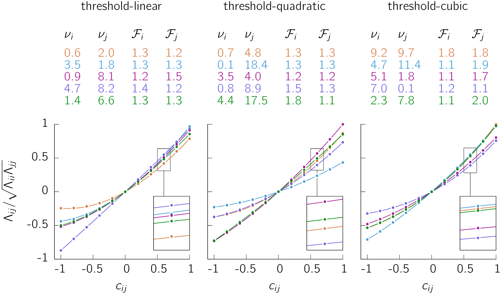
Figure 1: Numerical validation of our ansatz for rate covariances. Shown in 5 different colors are the results of 5 different simulations in which $\sqrt{\Sigma_{ii}}$ (resp. $\sqrt{\Sigma_{jj}}$) was drawn uniformly between $1$ and $4$, and $\mu_{i}$ (resp. $\mu_{j}$) was chosen so as to achieve a mean firing rate $\nu_{i}$ (resp. $\nu_{j}$) drawn from a Gamma distribution with a mean $5$ Hz and a shape parameter of $1$. Dots show $\Lambda_{ij}$ as a function of $c_{ij}$, as estimated via Monte-Carlo integration of Equation 39 with a million samples. Solid lines show Equation 40, which is by construction always exact at $c_{ij}=\pm 1$, and always has the right slope at $c_{ij}=0$. The corresponding tables show the mean firing rates and the Fano factors of both neurons (Fano factors were computed using Equation 54 with $\tau_{\rm A}=50$ ms and $T=100$ ms). The figures indicate that our approximation is highly accurate over a range of parameters corresponding to physiological values of firing rates and Fano factors. Parameters: $k=3$ (threshold-linear), $k=0.3$ (threshold-quadratic), $k=0.02$ (threshold-cubic).

The calculation of $\Lambda_{ij}(-1)$ is slightly more involved, but follows a similar logic. This time we assume that $\mu_{i}/\sqrt{\Sigma_{ii}}>-\mu_{j}/\sqrt{\Sigma_{jj}}$ (otherwise, $\Lambda_{ij}(-1)=0$), and we define

$$B_{ij}^{(n,m)}\equiv k^{2}\int\mathcal{D}u\ \lfloor\mu_{i}-u\sqrt{\Sigma_{ii}}\rfloor_{+}^{n}\ \lfloor\mu_{j}+u\sqrt{\Sigma_{jj}}\rfloor_{+}^{m}$$ (46)

Similar to Equation 45, we have the following recursive formula for $1<n\leq m$:

$$B_{ij}^{(n,m)}=\mu_{i}B_{ij}^{(n-1,m)}+(n-1)\Sigma_{ii}B_{ij}^{(n-2,m)}-m\sqrt{\Sigma_{ii}\Sigma_{jj}}B_{ij}^{(n-1,m-1)}$$ (47)

However, now the boundary conditions must also be computed recursively:

$$B_{ij}^{(0,m)} =\begin{cases}k^{2}\left[\psi_{i}+\psi_{j}-1\right]&{\rm if}\ m=0\\ \mu_{j}B_{ij}^{0,0}+k^{2}\sqrt{\Sigma_{jj}}\left(\phi_{j}-\phi_{i}\right)&{\rm if}\ m=1\\ \mu_{j}B_{ij}^{(0,m-1)}-\sqrt{\Sigma_{jj}}\left[k^{2}\phi_{i}R_{ij}^{m-1}-(m-1)\sqrt{\Sigma_{jj}}B_{ij}^{(0,m-2)}\right]&{\rm otherwise}\end{cases}$$ (48)

$$B_{ij}^{(1,m)} =\mu_{i}B_{ij}^{(0,m)}+\sqrt{\Sigma_{ii}}\begin{cases}k^{2}\left(\phi_{i}-\phi_{j}\right)&{\rm if}\ m=0\\ k^{2}\phi_{i}R_{ij}^{m}-m\sqrt{\Sigma_{jj}}B_{ij}^{(0,m-1)}&{\rm otherwise}\end{cases}$$ (49)

where we have used the shorthands $\phi_{\ell}\equiv\phi(\mu_{\ell}/\sqrt{\Sigma_{\ell\ell}})$, $\psi_{\ell}\equiv\psi(\mu_{\ell}/\sqrt{\Sigma_{\ell\ell}})$, and $R_{ij}\equiv\mu_{j}+\mu_{i}\sqrt{\Sigma_{jj}/\Sigma_{ii}}$.

Thus, $\Lambda_{ij}(c_{ij})$ is approximated in closed-form by a third-order polynomial in $c_{ij}$, given $\mu_{i}$, $\mu_{j}$, $\Sigma_{ii}$, $\Sigma_{jj}$ and $\Sigma_{ij}$. Our polynomial approximation is very accurate over a broad, physiologically relevant range of parameters (and in fact, even beyond that), for power law exponents in the physiological range (Figure 1).

In combination with the results of Section 2.2, we can then obtain the moments of $\mathbf{r}$, which we use in the following section to compute Fano factors and spike count correlations.

2.7 Spike count statistics

Under the assumption that each neuron $i$ emits spikes according to an inhomogeneous Poisson process with rate function $r_{i}(t)$ (“doubly stochastic”, or “Cox” process), we can compute the joint statistics of the spike counts in some time window, which is what electrophysiologists often report. Let $C_{i}^{T}(t)$ denote the number of spikes that are emitted by neuron $i$ in a window of duration $T$ starting at time $t$, and let $\kappa_{i}^{T}(t)=\int_{0}^{T}\mathrm{d}t\ r_{i}(t)$ be the expected number of spikes in that window, for a given trial and given the underlying rate trace $r_{i}(t)$. The Fano factor of the distribution of $C_{i}^{T}(t)$ is given by

$$\mathcal{F}_{i}^{T}(t)\quad=\quad\frac{{\rm var}\left[C_{i}^{T}(t)\right]}{{\rm mean}\left[C_{i}^{T}(t)\right]}\quad=\quad 1+\frac{{\rm var}\left[\kappa_{i}^{T}(t)\right]}{\langle\kappa_{i}^{T}(t)\rangle}$$ (50)

with

$$\langle\kappa_{i}^{T}(t)\rangle=\int_{0}^{T}\mathrm{d}t^{\prime}\>\nu_{i}(t+t^{\prime})$$ (51)

and

$${\rm var}\left[\kappa_{i}^{T}(t)\right]=\int_{0}^{T}\mathrm{d}s\int_{0}^{T}\mathrm{d}s^{\prime}\>\Lambda_{ii}(t+s,s^{\prime}-s)$$ (52)

All expected values such as $\nu_{i}$ and $\Lambda_{ii}$ have been calculated in previous sections. We approximate the integrals above by simple Riemann sums with a discretisation step of $1$ ms.

In the special case of constant input $\mathbf{h}$ leading to a stationary rate distribution, Equation 50 simplifies to

$$\mathcal{F}_{i}^{T}=1+\frac{1}{T\nu_{i}}\>\int_{0}^{T}\mathrm{d}s\int_{0}^{T}\mathrm{d}s^{\prime}\>\Lambda_{ii}(\cdot,s^{\prime}-s)$$ (53)

(the rate variance $\Lambda_{ii}(t,\tau)$ no longer depends on $t$, hence the notation $\Lambda_{ii}(\cdot,\tau)$). A closed-form approximation can be derived if the rate autocorrelation is well approximated by a Laplacian with decay time constant $\tau_{\rm A}$, i.e. $\Lambda_{ii}(\cdot,\tau)\approx\Lambda_{ii}(\cdot,0)\>\exp\left(-|\tau|/\tau_{\rm A}\right)$. In this case, Equation 53 evaluates to

$$\mathcal{F}_{i}^{T}\quad\approx\quad 1+\frac{2\>\tau_{\rm A}\>\Lambda_{ii}(\cdot,0)}{\nu_{i}}\left[1-\frac{\tau_{\rm A}}{T}\>\left(1-e^{-T/\tau_{\rm A}}\right)\right]$$ (54)

This expression is shown in Figure 2 as a function of the counting window $T$, for various autocorrelation lengths $\tau_{\sf A}$.

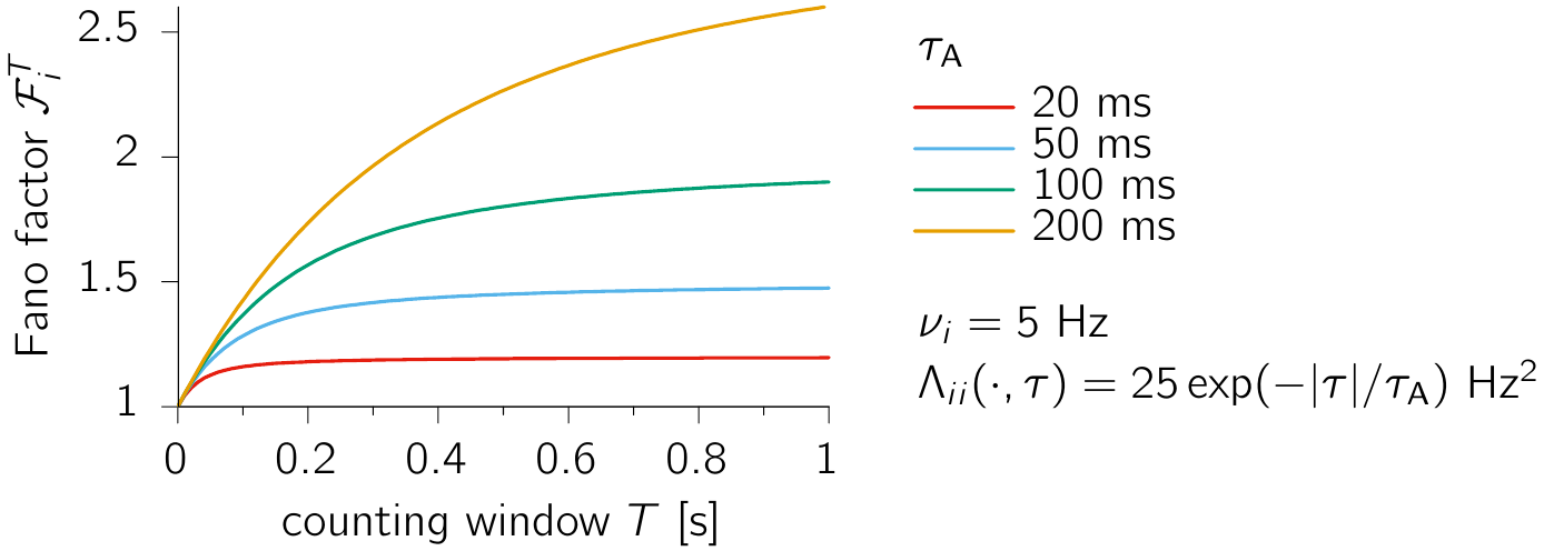
Figure 2: Approximation of the Fano factor when the autocorrelation is a Laplacian with time constant $\tau_{\sf A}$ (varied here; cf. color legend) – see also Equation 54.

The behaviour of $\mathcal{F}_{i}$ as a function of membrane potential sufficient statistics $\mu_{i}$ and $\sqrt{\Sigma_{ii}}$ is depicted in Figure 3, for various exponents of the threshold power-law gain function. In all cases (i.e. independent of the exponent $n$), the Fano factor grows with increasing potential variance. However, the dependence on $\mu_{i}$ strongly depends on $n$. For $n=1$, the Fano factor decreases with $\mu_{i}$, while for $n=3$ it increases. For $n=2$, the Fano factor has only a weak dependence on $\mu_{i}$. This behaviour can be understood qualitatively by linearising the gain function around the mean potential, which gives us an idea of how the super-Poisson part of the Fano factor depends on membrane potential statistics:

$$\mathcal{F}_{i}^{T}-1\propto n\mu_{i}^{n-2}\Sigma_{ii}$$ (55)

Therefore, the iso-Fano-factor lines in Figure 3 are expected to approximately obey $\sqrt{\Sigma_{ii}}\approx\mu_{i}^{2-n}$, which is roughly what we see from Figure 3.

It is instructive to plug in some typical numbers: assuming a mean firing rate of $\nu_{i}=5$ Hz, a counting window $T=50$ ms, a Fano factor $\mathcal{F}_{i}^{T}=1.5$ (characteristic of spontaneous activity in the cortex, Churchland et al.,, 2010), and an autocorrelation time constant $\tau_{\rm A}=40$ ms (Kenet et al.,, 2003; Berkes et al.,, 2011), then Equation 54 tells us that the fluctuations in $r_{i}$ must have a standard deviation of $\sqrt{\Lambda_{ii}}\simeq 8.5$ Hz. This is larger than the assumed mean firing rate ($5$ Hz), thus implying that the underlying rate variable in physiological conditions is often going to be zero, in turn implying that the membrane potential will often be found below the threshold of the firing rate nonlinearity $f(u)$. It is precisely in this regime that it becomes important to perform the nonlinear conversion of the moments of $\mathbf{u}$ into those of $\mathbf{r}$, taking into account the specific form of the nonlinearity; in that same regime, linearisation of the dynamics of Equation 1 can become very inaccurate.

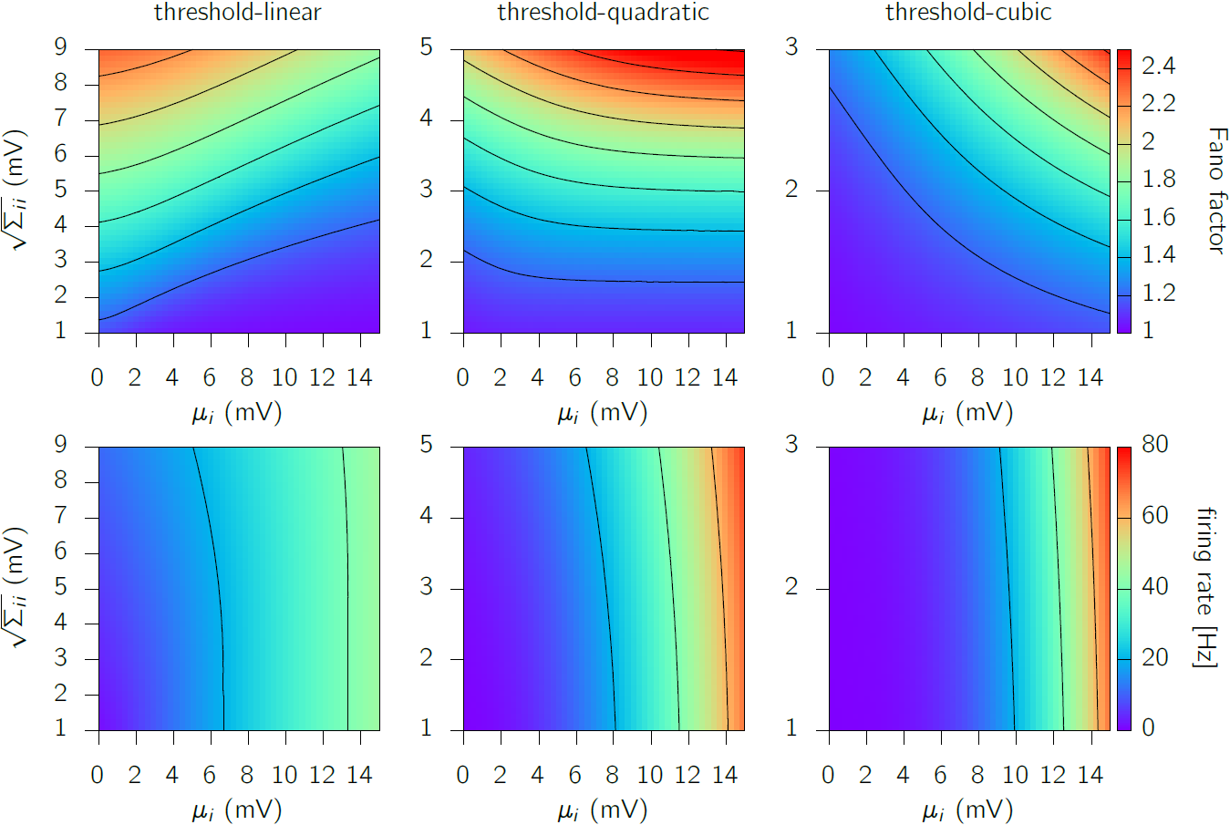
Figure 3: Fano factor $\mathcal{F}_{i}$ (top row) and mean firing rate $\nu_{i}$ (bottom row) as a function of membrane potential mean $\mu_{i}$ and standard deviation $\sqrt{\Sigma_{ii}}$, for $n=1$ to $n=3$ (left to right). To calculate $\mathcal{F}_{i}$, we used Equation 54, assuming an autocorrelation time constant of $\tau_{\rm A}=50$ ms. The multiplicative rescaling $k$ of the threshold power-law gain function was adjusted so that both Fano factors and firing rates span roughly the same range of values across $n=1$ to $n=3$, but the precise value of $k$ has no impact on the shape of the contour lines.

Similar derivations can be done for spike count correlations:

$$\rho_{ij}^{T}(t)\quad \equiv\quad\frac{{\rm cov}\left[C_{i}^{T}(t),C_{j}^{T}(t)\right]}{\sqrt{{\rm var}\left[\vphantom{C_{j}^{T}}C_{i}^{T}(t)\right]\ {\rm var}\left[C_{j}^{T}(t)\right]}}$$

$$=\quad\frac{\langle\kappa_{i}^{T}(t)\kappa_{j}^{T}(t)\rangle-\langle\kappa_{i}^{T}(t)\rangle\langle\kappa_{j}^{T}(t)\rangle}{\sqrt{\left({\rm var}\left[\vphantom{\kappa_{j}^{T}}\kappa_{i}^{T}(t)\right]+\langle\kappa_{i}^{T}(t)\rangle\right)\left({\rm var}\left[\kappa_{j}^{T}(t)\right]+\langle\kappa_{j}^{T}(t)\rangle\right)}}$$

$$=\quad\frac{\displaystyle\iint_{[0:T]^{2}}\mathrm{d}s\>\mathrm{d}s^{\prime}\ \Lambda_{ij}(t,s^{\prime}-s)}{\sqrt{\left({\rm var}\left[\vphantom{\kappa_{j}^{T}}\kappa_{i}^{T}(t)\right]+\langle\kappa_{i}^{T}(t)\rangle\right)\left({\rm var}\left[\kappa_{j}^{T}(t)\right]+\langle\kappa_{j}^{T}(t)\rangle\right)}}$$

$$=\left[\langle\kappa_{i}^{T}(t)\rangle\>\langle\kappa_{j}^{T}(t)\rangle\>\mathcal{F}_{i}^{T}(t)\>\mathcal{F}_{i}^{T}(t)\right]^{-\frac{1}{2}}\iint_{[0:T]^{2}}\mathrm{d}s\>\mathrm{d}s^{\prime}\ \Lambda_{ij}(t,s^{\prime}-s)$$ (56)

In the stationary case, Equation 56 becomes

$$\rho_{ij}^{T}\quad=\quad\frac{\displaystyle\iint_{[0:T]^{2}}\mathrm{d}s\>\mathrm{d}s^{\prime}\>\Lambda_{ij}(\cdot,s^{\prime}-s)}{T\>\sqrt{\nu_{i}\nu_{j}\mathcal{F}_{i}^{T}\mathcal{F}_{j}^{T}}}$$ (57)

3 Numerical validation

In this section, we demonstrate the validity of the equations derived in Section 2 on two examples: a random E/I network with weak and sparse connections, and a strongly connected, inhibition-stabilized E/I network.

3.1 Weakly connected random network

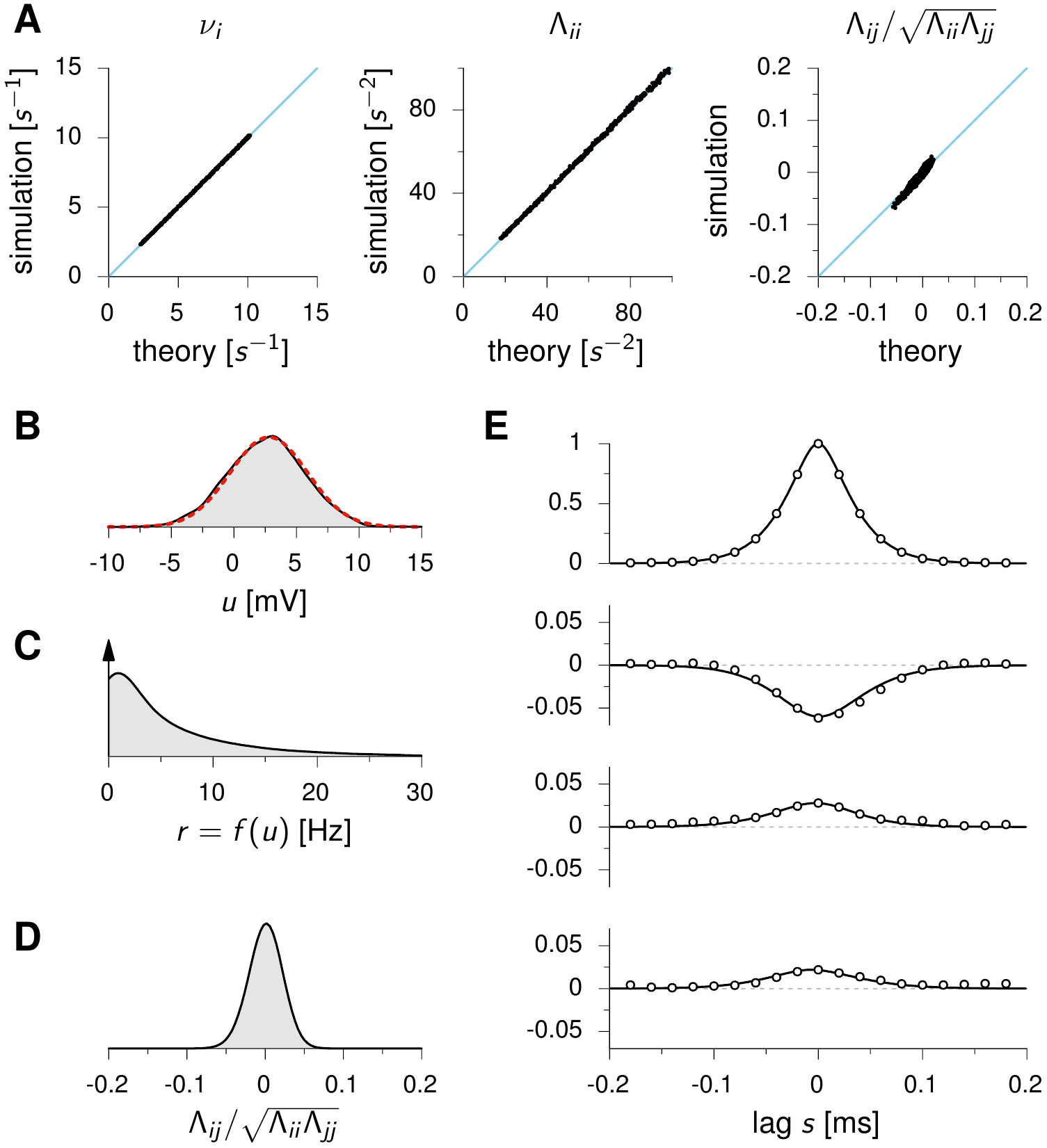
Figure 4: Validation of our theoretical results on a random, weakly connected E/I network. (A) Mean firing rates $\{\nu_{i}\}$, firing rate variances $\{\Lambda_{ii}\}$, and pairwise firing rate correlations, as predicted semi-analytically by the moment dynamics equations of Section 2 (x-axes) and compared to empirical estimates obtained from long stochastic simulations of Equation 25 (y-axes). (B) Distribution of membrane potentials $u_{i}(t)$ for a randomly chosen neuron (gray), and its Gaussian approximation $\mathcal{N}(u;\mu_{i},\Sigma_{ii})$ used in our theory. (C) Corresponding firing rate distribution of the same neuron as in (B). (D) Distribution of pairwise firing rate correlations across the network. (E) Example membrane potential normalized auto- (top row) and cross- (bottom rows) correlograms ($\Sigma_{ij}(\infty,s)/\sqrt{\Sigma_{ii}\Sigma_{jj}}$), as predicted by the theory (solid) and estimated from simulations (dots).

The network is made of $N_{\mathrm{E}}=250$ excitatory and $N_{\mathrm{I}}=250$ inhibitory neurons, each with a threshold-quadratic I/O nonlinearity: $f(u)=0.3\lfloor u\rfloor_{+}^{2}$. We set all intrinsic time constants to $\tau_{i}=\tau\equiv 20$ ms. The input noise has no spatial, but only temporal, correlations:

$$\langle\eta_{i}(t)\eta_{j}(t+s)\rangle=\frac{\sigma_{0}^{2}}{1+\tau/\tau_{\eta}}\>\exp\left(-\frac{|s|}{\tau_{\eta}}\right)\delta_{ij}$$ (58)

with $\tau_{\eta}=50$ ms and $\sigma_{0}=3$ mV representing the standard deviation of the membrane potentials if the recurrent connectivity were removed. Synaptic weights are drawn randomly from the following distribution:

$$W_{ij}=\frac{\alpha s_{j}}{\sqrt{N}}\times\left\{\begin{array}[]{rl}1&\text{with probability 0.2}\\ 0&\text{otherwise}\end{array}\right.$$ (59)

where $\alpha$ is a global scaling factor (see below), $s_{j}$ is a presynaptic signed factor equal to $+1$ if neuron $j$ is excitatory ($1\leq j\leq N/2$), and equal to $-\gamma$ if neuron $j$ is inhibitory ($N/2<j\leq N$). We set $\gamma=3$ to place the network in the inhibition-dominated regime where the average pairwise correlation among neurons is weak (Renart et al.,, 2010; Hennequin et al.,, 2012). The scaling factor $\alpha=2.2$ was chosen such that the network is effectively weakly connected and thus far from instability.

The network is fed with a constant input $\mathbf{h}=\mathbf{u^{\star}}-\mathbf{W}f(\mathbf{u}^{\star})$, such that, in the absence of stochasticity, the network would have a (stable) fixed point at $\mathbf{u}=\mathbf{u}^{\star}$ – we drew the elements of $\mathbf{u}^{\star}$ from a uniform distribution between $1$ and $4$ mV.

We simulated the stochastic dynamics of the network (Equation 25) for $5000$ seconds, and computed empirical estimates of the moments in the steady-state, stationary regime (mean firing rates, firing rate variances, firing rate correlations, and full membrane potential cross-correlograms). We found those estimates to agree very well with the semi-analytical solutions obtained by integrating the relevant equations of motion derived in Section 2 under the Gaussian assumption (Figure 4A). Membrane potentials are indeed roughly normally distributed (Figure 4B), with a standard deviation on the same order as the mean, yielding very skewed distributions of firing rates (Figure 4C). Due to the effectively weak connectivity, pairwise correlations among firing rate fluctuations are weak in magnitude (Figure 4D). Membrane potential cross-correlograms have a simple, near-symmetric structure (random, weakly connected networks are close to equilibrium) and are well captured by the theory.

3.2 Strongly connected, inhibition-stabilized random network

We now consider a strongly connected E/I network much further away from equilibrium than the weakly-connected network of Figure 4. This network operates in the inhibition-stabilized regime, whereby excitatory feedback is strongly distabilizing on its own, but is dynamically stabilized by feedback inhibition. The details of how we obtained such a network are largely irrelevant here (but see Hennequin et al.,, 2014). All the parameters of the network will be posted online together with the code to ensure reproducibility.

Our results are summarized in Figure 5, in exactly the same format as in Figure 4. This network strongly amplifies the input noise process along a few specific directions in state space, leading to strong (negative and positive) pairwise correlations among neuronal firing rates Figure 5D. Thus, the central limit theorem – which would in principle justify our core assumption that membrane potentials are jointly Gaussian, as large (and low-pass-filtered) sums of uncorrelated variables – may not apply. Indeed, most membrane potential distributions have substantial (negative) skewness (Figure 5B), leading to some inaccuracies in our semi-analytical calculation of the moments (Figure 5A), which we find are reasonably small nonetheless. We leave the extension of our theory to third-order moments (e.g. Dahmen et al.,, 2016) for future work. Finally, the strong connectivity gives rise to non-trivial temporal structure in the joint activity of pairs of neurons reflecting non-equilibrium dynamics. Even in this regime, our results capture the membrane potential cross-correlograms well (Figure 5E).

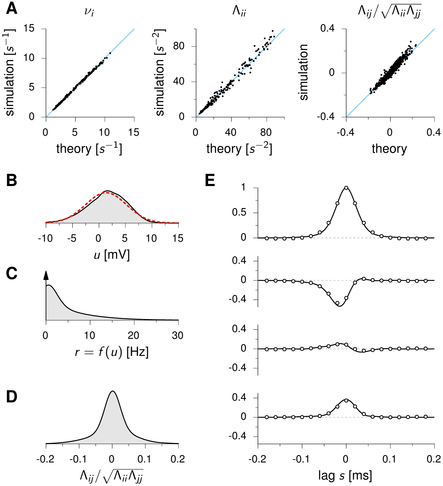
Figure 5: Validation of our theoretical results on a random, strongly connected, inhibition-stabilized E/I network. The figure follows the same format as in Figure 4 above; see caption there.

References

- Ahmadian et al., (2013) Ahmadian, Y., Rubin, D. B., and Miller, K. D. (2013). Analysis of the stabilized supralinear network. Neural Comput., 25:1994–2037.
- Barrett, (2012) Barrett, D. (2012). Computation in balanced networks. PhD thesis, University College London.
- Berkes et al., (2011) Berkes, P., Orbán, G., Lengyel, M., and Fiser, J. (2011). Spontaneous cortical activity reveals hallmarks of an optimal internal model of the environment. Science, 331(6013):83–87.
- Bonnabel and Sepulchre, (2012) Bonnabel, S. and Sepulchre, R. (2012). The geometry of low-rank Kalman filters. arXiv:1203.4049 [cs, math].
- Buesing et al., (2012) Buesing, L., Macke, J., and Sahani, M. (2012). Spectral learning of linear dynamics from generalised-linear observations with application to neural population data. In Advances in Neural Information Processing Systems 25, pages 1691–1699.
- Churchland et al., (2010) Churchland, M. M., Yu, B. M., Cunningham, J. P., Sugrue, L. P., Cohen, M. R., Corrado, G. S., Newsome, W. T., Clark, A. M., Hosseini, P., Scott, B. B., Bradley, D. C., Smith, M. A., Kohn, A., Movshon, J. A., Armstrong, K. M., Moore, T., Chang, S. W., Snyder, L. H., Lisberger, S. G., Priebe, N. J., Finn, I. M., Ferster, D., Ryu, S. I., Santhanam, G., Sahani, M., and Shenoy, K. V. (2010). Stimulus onset quenches neural variability: a widespread cortical phenomenon. Nat Neurosci, 13(3):369–378.
- Dahmen et al., (2016) Dahmen, D., Bos, H., and Helias, M. (2016). Correlated fluctuations in strongly coupled binary networks beyond equilibrium. Phys. Rev. X, 6(3):031024.
- Gardiner, (1985) Gardiner, C. W. (1985). Handbook of stochastic methods: for physics, chemistry, and the natural sciences. Berlin: Springer.
- Hennequin et al., (2016) Hennequin, G., Ahmadian⋆, Y., Rubin⋆, D. B., Lengyel†, M., and Miller†, K. D. (2016). Stabilized supralinear network dynamics account for stimulus-induced changes of noise variability in the cortex. Submitted.
- Hennequin et al., (2012) Hennequin, G., Vogels, T. P., and Gerstner, W. (2012). Non-normal amplification in random balanced neuronal networks. Phys. Rev. E, 86:011909.
- Hennequin et al., (2014) Hennequin, G., Vogels, T. P., and Gerstner, W. (2014). Optimal control of transient dynamics in balanced networks supports generation of complex movements. Neuron, 82:1394–1406.
- Kenet et al., (2003) Kenet, T., Bibitchkov, D., Tsodyks, M., Grinvald, A., and Arieli, A. (2003). Spontaneously emerging cortical representations of visual attributes. Nature, 425(6961):954–956.
- Miller and Troyer, (2002) Miller, K. D. and Troyer, T. W. (2002). Neural noise can explain expansive, power-law nonlinearities in neural response functions. J. Neurophysiol., 87(2):653–659.
- Murphy and Miller, (2009) Murphy, B. K. and Miller, K. D. (2009). Balanced amplification: A new mechanism of selective amplification of neural activity patterns. Neuron, 61:635–648.
- Priebe et al., (2004) Priebe, N. J., Mechler, F., Carandini, M., and Ferster, D. (2004). The contribution of spike threshold to the dichotomy of cortical simple and complex cells. Nat. Neurosci., 7(10):1113–1122.
- Renart et al., (2010) Renart, A., de la Rocha, J., Bartho, P., Hollender, L., Parga, N., Reyes, A., and Harris, K. (2010). The asynchronous state in cortical circuits. Science, 327:587.
- Rubin et al., (2015) Rubin, D., Van Hooser, S., and Miller, K. (2015). The stabilized supralinear network: A unifying circuit motif underlying multi-input integration in sensory cortex. Neuron, 85(2):402–417.