Computer simulations of melts of randomly branching polymers

Angelo Rosa anrosa@sissa.it Sissa (Scuola Internazionale Superiore di Studi Avanzati), Via Bonomea 265, 34136 Trieste, Italy    Ralf Everaers ralf.everaers@ens-lyon.fr Univ Lyon, Ens de Lyon, Univ Claude Bernard Lyon 1, CNRS, Laboratoire de Physique and Centre Blaise Pascal, F-69342 Lyon, France
Abstract

Randomly branching polymers with annealed connectivity are model systems for ring polymers and chromosomes. In this context, the branched structure represents transient folding induced by topological constraints. Here we present computer simulations of melts of annealed randomly branching polymers of 3N18003𝑁18003\leq N\leq 1800 segments in d=2𝑑2d=2 and d=3𝑑3d=3 dimensions. In all cases, we perform a detailed analysis of the observed tree connectivities and spatial conformations. Our results are in excellent agreement with an asymptotic scaling of the average tree size of RN1/dsimilar-to𝑅superscript𝑁1𝑑R\sim N^{1/d}, suggesting that the trees behave as compact, territorial fractals. The observed swelling relative to the size of ideal trees, RN1/4similar-to𝑅superscript𝑁14R\sim N^{1/4}, demonstrates that excluded volume interactions are only partially screened in melts of annealed trees. Overall, our results are in good qualitative agreement with the predictions of Flory theory. In particular, we find that the trees swell by the combination of modified branching and path stretching. However, the former effect is subdominant and difficult to detect in d=3𝑑3d=3 dimensions.

preprint: AIP/123-QED

I Introduction

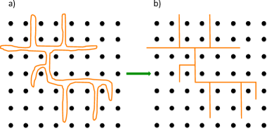
Randomly branched polymers or trees display surprisingly rich physics. In Statistical Mechanics, lattice trees are believed to fall into the same universality class as lattice animals IsaacsonLubensky ; SeitzKlein1981 ; DuarteRuskin1981 and their critical exponents are related to those of magnetic systems ParisiSourlasPRL1981 ; FisherPRL1978 ; KurtzeFisherPRB1979 ; BovierFroelichGlaus1984 . In Polymer Chemistry, the deliberate (or accidental Read2013 ) incorporation of monomers with higher functionality into the polymerisation processes modifies materials properties RubinsteinColby ; Burchard1999 . In this context, one has to distinguish the environmental conditions under which chains are studied from those under which they are synthesised and where their connectivity is said to be quenched. Here we are interested in randomly branched polymers with annealed connectivity, whose structure is meant to represent the transient folding of topologically constrained ring polymers KhokhlovNechaev85 ; RubinsteinPRL1986 ; RubinsteinPRL1994 ; kapnistos2008 ; GrosbergSoftMatter2014 ; RosaEveraersPRL2014 ; Rosa2016a (Fig. 1) and chromosomes grosbergEPL1993 ; RosaPLOS2008 ; Vettorel2009 ; MirnyRev2011 . At the light of the recent results by Lang LangMacromol2013 and Smrek and Grosberg SmrekGrosbergACSMacroLett2016 who analysed the threadable fraction of the minimal area encircled by non-concatenated ring polymers in melt, it is a non-trivial and still open question, if CatesDeutsch or to which extent RubinsteinPRL1994 ; RubinsteinMacromolecules2016 this analogy KhokhlovNechaev85 holds also for these systems. However, having shown that it provides at least an excellent approximation RosaEveraersPRL2014 , we now proceed to analyse in some detail the statistical properties of melts of annealed trees.
Refer to caption
Figure 1: Behaviour of a two-dimensional ring (orange) in an array of impenetrable fixed obstacles (schematically represented by the black dots). To maximize its conformational entropy, the ring adopts a transiently branched shape (a), which can then be mapped to a lattice tree (b) with annealed connectivity. The figure is adapted from kapnistos2008 .

As customary in polymer physics DeGennesBook ; DoiEdwards ; KhokhlovGrosberg ; RubinsteinColby , we are primarily interested in exponents describing how expectation values for observables scale with the weight, N𝑁N, of the trees:

Nbr(N)delimited-⟨⟩subscript𝑁𝑏𝑟𝑁\displaystyle\langle N_{br}(N)\rangle similar-to\displaystyle\sim Nϵsuperscript𝑁italic-ϵ\displaystyle N^{\epsilon} (1)
L(N)delimited-⟨⟩𝐿𝑁\displaystyle\langle L(N)\rangle similar-to\displaystyle\sim Nρsuperscript𝑁𝜌\displaystyle N^{\rho} (2)
Rg2(N)delimited-⟨⟩superscriptsubscript𝑅𝑔2𝑁\displaystyle\langle R_{g}^{2}(N)\rangle similar-to\displaystyle\sim N2νsuperscript𝑁2𝜈\displaystyle N^{2\nu} (3)

or the path distance l𝑙l between tree nodes:

R2(l)delimited-⟨⟩superscript𝑅2𝑙\displaystyle\langle R^{2}(l)\rangle similar-to\displaystyle\sim l2νpathsuperscript𝑙2subscript𝜈path\displaystyle l^{2\nu_{\mathrm{path}}} (4)
pc(l)delimited-⟨⟩subscript𝑝𝑐𝑙\displaystyle\langle p_{c}(l)\rangle similar-to\displaystyle\sim lνpath(d+θpath)superscript𝑙subscript𝜈path𝑑subscript𝜃path\displaystyle l^{-\nu_{\mathrm{path}}(d+\theta_{\mathrm{path}})} (5)

Here, Nbr(N)delimited-⟨⟩subscript𝑁𝑏𝑟𝑁\langle N_{br}(N)\rangle denotes the average branch weight; L(N)delimited-⟨⟩𝐿𝑁\langle L(N)\rangle the average contour distance or length of paths on the tree; Rg2(N)delimited-⟨⟩superscriptsubscript𝑅𝑔2𝑁\langle R_{g}^{2}(N)\rangle the mean-square gyration radius of the trees; and R2(l)delimited-⟨⟩superscript𝑅2𝑙\langle R^{2}(l)\rangle and pc(l)delimited-⟨⟩subscript𝑝𝑐𝑙\langle p_{c}(l)\rangle the mean-square spatial distance and contact probability of nodes as a function of their contour distance, l𝑙l. For ideal, non-interacting trees ZimmStockmayer49 ; Rosa2016a ρ=ϵ=νpath=1/2𝜌italic-ϵsubscript𝜈path12\rho=\epsilon=\nu_{\mathrm{path}}=1/2, ν=1/4𝜈14\nu=1/4 and θpath=0subscript𝜃path0\theta_{\mathrm{path}}=0. For interacting systems, the only exactly known exponent is ν=1/2𝜈12\nu=1/2 for self-avoiding trees in d=3𝑑3d=3 dimensions ParisiSourlasPRL1981 . Flory theory provides a simple and insightful description of a wide range of interacting tree systems IsaacsonLubensky ; DaoudJoanny1981 ; GutinGrosberg93 ; GrosbergSoftMatter2014 , but the results are obtained through uncontrolled approximations and rely on the cancellation of large errors  DeGennesBook ; DesCloizeauxBook . For the present problem, Flory theory predicts that trees in a melt ought to behave as compact fractals with Rg2(N)N2/dsimilar-todelimited-⟨⟩superscriptsubscript𝑅𝑔2𝑁superscript𝑁2𝑑\langle R_{g}^{2}(N)\rangle\sim N^{2/d} and that trees should swell by a combination of path swelling and modified branching. As plausible as this prediction might be, it needs to be corroborated by more rigorous approaches.

Here we present the, to our knowledge, first computational study of the properties of melts of annealed trees in d=2𝑑2d=2 and d=3𝑑3d=3 dimensions. The article is part of a series Everaers2016a ; Everaers2016b ; Rosa2016a ; Rosa2016c , where we use a combination of computer simulations, Flory theory and scaling arguments to investigate the connectivity and conformational statistics of randomly branched polymers with excluded volume interactions. We employ the same notation, definitions and numerical methodologies introduced in our previous work Rosa2016a on single self-avoiding trees in good solvent, which we briefly summarise in Sections II and III. Results for trees connectivity and spatial conformations are outlined in Sec. IV and discussed in detail in Sec. V. Finally, conclusions are sketched in Sec. VI.

II Model and Background

We are interested in randomly branched polymers with annealed connectivity and repulsive, short-range interactions between monomers. Secs. II.1 and II.2 summarize our choices of the employed lattice model, units and notation and the definition of observables. Sec. II.3 reviews predictions of Flory theory for interacting trees. Finally, Secs. II.4 and II.5 provide a justification for the model parameters and the sizes of simulated trees by employing the concept of “blob size”. All our numerical results are obtained for trees embedded in d=2𝑑2d=2 and d=3𝑑3d=3 dimensions, even though many theoretical expressions are conveniently expressed for general d𝑑d.

II.1 Model

We study lattice trees on the 2d2𝑑2d- and 3d3𝑑3d-cubic lattice. The functionality of the nodes is restricted to the values f=1𝑓1f=1 (a leaf or branch tip), f=2𝑓2f=2 (linear chain section), and f=3𝑓3f=3 (branch point). Connected nodes occupy adjacent lattice sites. A tree conformation, 𝒯(𝒢,Γ)𝒯𝒢Γ{\cal T}\equiv({\mathcal{G}},\Gamma), can be described by the set of node positions, Γ={r1,,rN+1}Γsubscript𝑟1subscript𝑟𝑁1\Gamma=\{\vec{r}_{1},\dots,\vec{r}_{N+1}\}, in the embedding space and a suitable representation of its connectivity graph, 𝒢𝒢{\mathcal{G}}. We employ a data structure in the form of a linked list, which retains for each node, i𝑖i, its position, risubscript𝑟𝑖\vec{r}_{i}, functionality, fisubscript𝑓𝑖f_{i}, and the indices {j1(i),,jfi(i)}subscript𝑗1𝑖subscript𝑗subscript𝑓𝑖𝑖\{j_{1}(i),\ldots,j_{f_{i}}(i)\} of the nodes to which it is connected.

Since our models do not include a bending energy, the lattice constant equals the Kuhn length, lKsubscript𝑙𝐾l_{K}, of linear paths across ideal trees. We measure energy in units of kBTsubscript𝑘𝐵𝑇k_{B}T, length in units of the lattice constant or Kuhn length, lKsubscript𝑙𝐾l_{K}, and mass in units of the number of Kuhn segments. Similarly, we specify the density by the Kuhn segment number density, ρKsubscript𝜌𝐾\rho_{K}. We use the letters N𝑁N and n𝑛n to denote the mass of a tree or a branch, respectively. With N𝑁N Kuhn segments connecting the nodes of a tree, there are N+1𝑁1N+1 nodes in a tree. The symbols L𝐿L and l𝑙l are reserved for contour lengths of linear paths on the tree, while δL𝛿𝐿\delta L and δl𝛿𝑙\delta l denote contour distances from a fixed point, typically the tree center. Spatial distances are denoted by the letters R𝑅R and r𝑟r. Examples are the tree gyration radius, Rgsubscript𝑅𝑔R_{g}, spatial distances between nodes, rijsubscript𝑟𝑖𝑗\vec{r}_{ij}, and the spatial distances, δrisubscript𝛿𝑟𝑖\vec{\delta r}_{i}, of a node from the tree center of mass.

For ideal trees, nodes do not interact and their asymptotic branching probability, λ𝜆\lambda, is controlled via a chemical potential for branch points,

id(𝒯)=μbrn3(𝒢)subscript𝑖𝑑𝒯subscript𝜇𝑏𝑟subscript𝑛3𝒢{\mathcal{H}}_{id}({\cal T})=\mu_{br}n_{3}({\mathcal{G}}) (6)

where n3(𝒢)subscript𝑛3𝒢n_{3}({\mathcal{G}}) is the total number of 3-functional nodes in the tree. All our results are obtained RosaEveraersPRL2014 for a value of μbr=2.0kBTsubscript𝜇𝑏𝑟2.0subscript𝑘𝐵𝑇\mu_{br}=-2.0\,k_{B}T. Interactions between nodes are accounted for via

int(𝒯)=vKilatticenK,i2subscript𝑖𝑛𝑡𝒯subscript𝑣𝐾subscript𝑖𝑙𝑎𝑡𝑡𝑖𝑐𝑒superscriptsubscript𝑛𝐾𝑖2{\mathcal{H}}_{int}({\cal T})=v_{K}\sum_{i\in lattice}n_{K,i}^{2} (7)

where nK,isubscript𝑛𝐾𝑖n_{K,i} is the total number of Kuhn segments inside the elementary cell centered at the lattice site i𝑖i. In all cases we employ the same, large free energy penalty of vK=4kBTsubscript𝑣𝐾4subscript𝑘𝐵𝑇v_{K}=4\,k_{B}T for overlapping pairs of Kuhn segments, Eq. (7). The pair repulsion is so strong, that single trees are effectively self-avoiding, while the local occupancy fluctuations in our melts is (nK,inK,i)20.120.13delimited-⟨⟩superscriptsubscript𝑛𝐾𝑖delimited-⟨⟩subscript𝑛𝐾𝑖20.120.13\langle(n_{K,i}-\langle n_{K,i}\rangle)^{2}\rangle\approx 0.12-0.13 for all densities.

II.2 Observables

A tree is a branched structure free of loops. Its connectivity can be characterized in a number of ways. Locally, nodes connecting Kuhn segments differ according to their functionality, f𝑓f, with branch points having functionality f3𝑓3f\equiv 3 and branch tips f1𝑓1f\equiv 1. Given nfsubscript𝑛𝑓n_{f} the total number of tree nodes with functionality f𝑓f, they satisfy the relations:

n1subscript𝑛1\displaystyle n_{1} =\displaystyle= 2+n32subscript𝑛3\displaystyle 2+n_{3} (8)
n2subscript𝑛2\displaystyle n_{2} =\displaystyle= N12n3𝑁12subscript𝑛3\displaystyle N-1-2n_{3} (9)

For our choice of parameters, ideal trees are characterized by an asymptotic branching probability Rosa2016a

λ=limNn3(N)N=0.4𝜆subscript𝑁delimited-⟨⟩subscript𝑛3𝑁𝑁0.4\lambda=\lim_{N\rightarrow\infty}\langle\frac{n_{3}(N)}{N}\rangle=0.4 (10)

The large scale structure of a tree can be analyzed in terms of the ensemble of sub-trees generated by cutting bonds. Removal of a bond splits a tree of weight N𝑁N into two trees of weight n𝑛n and N1n𝑁1𝑛N-1-n. Defining Nbrmin(n,N1n)subscript𝑁𝑏𝑟𝑛𝑁1𝑛N_{br}\equiv\min(n,N-1-n) as the branch weight, the corresponding ensemble average grows as a characteristic power of the tree weight, Nbr(N)Nϵsimilar-todelimited-⟨⟩subscript𝑁𝑏𝑟𝑁superscript𝑁italic-ϵ\langle N_{br}(N)\rangle\sim N^{\epsilon} (Eq. (1)).

Alternatively, the tree connectivity can be analyzed in terms of: (1) the statistics of minimal distances, lijsubscript𝑙𝑖𝑗l_{ij}, of two nodes i,j𝑖𝑗i,j along linear paths on the tree, and its corresponding ensemble average L(N)delimited-⟨⟩𝐿𝑁\langle L(N)\rangle; (2) the average distance, δLcenter(N)delimited-⟨⟩𝛿subscript𝐿center𝑁\langle\delta L_{\mathrm{center}}(N)\rangle of nodes from the central node; (3) the average length δLcentermax(N)delimited-⟨⟩𝛿superscriptsubscript𝐿centermax𝑁\langle\delta L_{\mathrm{center}}^{\mathrm{max}}(N)\rangle of the longest distance from the central node. For ensemble averages one expects (Eq. (2)): L(N)δLcenterδLcentermax(N)Nρsimilar-todelimited-⟨⟩𝐿𝑁delimited-⟨⟩𝛿subscript𝐿centersimilar-todelimited-⟨⟩𝛿superscriptsubscript𝐿centermax𝑁similar-tosuperscript𝑁𝜌\langle L(N)\rangle\sim\langle\delta L_{\mathrm{center}}\rangle\sim\langle\delta L_{\mathrm{center}}^{\mathrm{max}}(N)\rangle\sim N^{\rho} with MadrasJPhysA1992 ρ=ϵ𝜌italic-ϵ\rho=\epsilon. Similarly, we characterize the statistics of branches by measuring the average branch weight, Nbr(δlrootmax)delimited-⟨⟩subscript𝑁𝑏𝑟𝛿superscriptsubscript𝑙rootmax\langle N_{br}(\delta l_{\mathrm{root}}^{\mathrm{max}})\rangle, as a function of the longest contour distance of nodes from the branch root, δlrootmax(Nbr)𝛿superscriptsubscript𝑙rootmaxsubscript𝑁𝑏𝑟\delta l_{\mathrm{root}}^{\mathrm{max}}(N_{br}). Finally, we consider the average weight of the “core” of tree, Ncenter(δlcenter)delimited-⟨⟩subscript𝑁𝑐𝑒𝑛𝑡𝑒𝑟𝛿subscript𝑙center\langle N_{center}(\delta l_{\mathrm{center}})\rangle, made of segments whose distance from the central node does not exceed δlcenter𝛿subscript𝑙center\delta l_{\mathrm{center}}.

The overall spatial extension of the tree is best described through the mean-square gyration radius Rg2delimited-⟨⟩superscriptsubscript𝑅𝑔2\langle R_{g}^{2}\rangle which is the average square distance of a node from the tree center of mass. Asymptotically, it is expected to scale as Rg2N2νsimilar-todelimited-⟨⟩superscriptsubscript𝑅𝑔2superscript𝑁2𝜈\langle R_{g}^{2}\rangle\sim N^{2\nu} (Eq. (3)).

The spatial conformations of linear paths of length l𝑙l on trees of total mass N𝑁N can be characterized using standard observables for linear polymers, namely: (1) the mean-square end-to-end distance R2(l,N)delimited-⟨⟩superscript𝑅2𝑙𝑁\langle R^{2}(l,N)\rangle; (2) for a given contact distance rcsubscript𝑟𝑐r_{c}, the corresponding end-to-end closure probability pc(l,N)delimited-⟨⟩subscript𝑝𝑐𝑙𝑁\langle p_{c}(l,N)\rangle. They are expected to scale, respectively, as (Eqs. (4) and (5)): R2(l)l2νpathsimilar-todelimited-⟨⟩superscript𝑅2𝑙superscript𝑙2subscript𝜈path\langle R^{2}(l)\rangle\sim l^{2\nu_{\mathrm{path}}} and pc(l)lνpath(d+θpath)similar-todelimited-⟨⟩subscript𝑝𝑐𝑙superscript𝑙subscript𝜈path𝑑subscript𝜃path\langle p_{c}(l)\rangle\sim l^{-\nu_{\mathrm{path}}(d+\theta_{\mathrm{path}})} and to be asymptotically independent of tree weight. By construction Rosa2016a , ν=νpathρ𝜈subscript𝜈path𝜌\nu=\nu_{\mathrm{path}}\,\rho.

II.3 Flory theory

Flory theories FloryChemBook are formulated as a balance of an entropic elastic term and an interaction energy:

=el+inter.subscript𝑒𝑙subscript𝑖𝑛𝑡𝑒𝑟{\mathcal{F}}={\mathcal{F}_{el}}+{\mathcal{F}_{inter}}\,. (11)

The central element of the Flory theory of interacting trees is the elastic free energy of ideal annealed trees GutinGrosberg93 ; GrosbergNechaev2015 ,

elkBTR2lKL+L2NlK2,similar-tosubscript𝑒𝑙subscript𝑘𝐵𝑇superscript𝑅2subscript𝑙𝐾𝐿superscript𝐿2𝑁superscriptsubscript𝑙𝐾2\frac{{\mathcal{F}}_{el}}{k_{B}T}\sim\frac{R^{2}}{l_{K}L}+\frac{L^{2}}{N\,l_{K}^{2}}\ , (12)

Ensembles of quenched trees are characterised by fixed values of LlKNρsimilar-to𝐿subscript𝑙𝐾superscript𝑁𝜌L\sim l_{K}N^{\rho} and the Flory energy needs to be minimized over R𝑅R. Linear chains represent a special case, where L=lKN𝐿subscript𝑙𝐾𝑁L=l_{K}N. In annealed trees, interactions can modify the branching statistics as well as the spatial conformations. With larger contour distances leading to larger spatial distances between repelling monomers, the Flory energy needs to be simultaneously minimized over both variables, R𝑅R and L𝐿L. Optimising L𝐿L for a given size, RNνsimilar-to𝑅superscript𝑁𝜈R\sim N^{\nu}, yields

ρ𝜌\displaystyle\rho =\displaystyle= 1+2ν312𝜈3\displaystyle\frac{1+2\nu}{3} (13)

and

νpathsubscript𝜈path\displaystyle\nu_{\mathrm{path}} =\displaystyle= 3ν1+2ν.3𝜈12𝜈\displaystyle\frac{3\nu}{1+2\nu}\ . (14)

Thus independently of the physical origin of the effect, swollen trees with ν>νideal1/4𝜈superscript𝜈ideal14\nu>\nu^{\mathrm{ideal}}\equiv 1/4 are predicted to display both, modified connectivities with ρ>ρideal1/2𝜌superscript𝜌ideal12\rho>\rho^{\mathrm{ideal}}\equiv 1/2 and path swelling with νpath>νpathideal1/2subscript𝜈pathsubscriptsuperscript𝜈idealpath12\nu_{\mathrm{path}}>\nu^{\mathrm{ideal}}_{\mathrm{path}}\equiv 1/2.

In melts, volume interactions are screened IsaacsonLubensky ; GrosbergSoftMatter2014 and dominated by high-order collisions of dense systems. Inspecting all terms of order p𝑝p in a (standard) virial-type expansion of the interaction energy term in Eq. (11DaoudJoanny1981 :

inter(N,R)(NRd)p1,similar-tosubscript𝑖𝑛𝑡𝑒𝑟𝑁𝑅superscript𝑁superscript𝑅𝑑𝑝1{\mathcal{F}_{inter}(N,R)}\sim\left(\frac{N}{R^{d}}\right)^{p-1}\,, (15)

shows that interactions are estimated to be irrelevant, if νd>1𝜈𝑑1\nu d>1. Even without swelling, this is the case in d>4𝑑4d>4 dimensions, where νideald=d/4>1superscript𝜈ideal𝑑𝑑41\nu^{\mathrm{ideal}}d=d/4>1 suggests ideal tree behavior. In d4𝑑4d\leq 4 dimensions, for 1/4<ν1/d14𝜈1𝑑1/4<\nu\leq 1/d the series is dominated by the p𝑝p\rightarrow\infty limit. Minimising the sum of Eqs. (12) and (15) in this limit with respect to L𝐿L and R𝑅R yields:

ν𝜈\displaystyle\nu =\displaystyle= 1d1𝑑\displaystyle\frac{1}{d} (16)
νpathsubscript𝜈path\displaystyle\nu_{\mathrm{path}} =\displaystyle= 3d+23𝑑2\displaystyle\frac{3}{d+2} (17)
ρ𝜌\displaystyle\rho =\displaystyle= d+23d𝑑23𝑑\displaystyle\frac{d+2}{3d} (18)

Eqs. (16) to (18) predict that in the melt state annealed trees are compact fractals. Interestingly, νpathsubscript𝜈path\nu_{\mathrm{path}} has the same value as the critical exponent ν𝜈\nu for linear self-avoiding walks, suggesting a deeper analogy between the two problems GrosbergSoftMatter2014 .

II.4 Blob size

Assuming that entropic effects are too small to induce density inhomogeneities, we can estimate the asymptotic behaviour from the assumption RubinsteinPRL1994 that the asymptotic segment self density at the tree center of mass converges to the melt segment density ρKsubscript𝜌𝐾\rho_{K}. More precisely RosaEveraersPRL2014 , ϕ(ρtree(2π)ddet(S))1N/Rd/ρK1italic-ϕsuperscriptsubscript𝜌𝑡𝑟𝑒𝑒superscript2𝜋𝑑𝑆1similar-to𝑁superscript𝑅𝑑subscript𝜌𝐾1\phi\equiv\left(\rho_{tree}\sqrt{(2\pi)^{d}\det(S)}\right)^{-1}\sim N/R^{d}/\rho_{K}\rightarrow 1, where S𝑆S is the gyration or shape tensor, Sαβ=1N+1i=1N+1(riαrCM,α)(riβrCM,β)subscript𝑆𝛼𝛽1𝑁1superscriptsubscript𝑖1𝑁1subscript𝑟𝑖𝛼subscript𝑟𝐶𝑀𝛼subscript𝑟𝑖𝛽subscript𝑟𝐶𝑀𝛽S_{\alpha\beta}=\frac{1}{N+1}\sum_{i=1}^{N+1}(\vec{r}_{i\alpha}-\vec{r}_{CM,\alpha})(\vec{r}_{i\beta}-\vec{r}_{CM,\beta}) and rCMsubscript𝑟𝐶𝑀\vec{r}_{CM} is the spatial position of the tree centre of mass. Neglecting asphericity,

Rg2(N)meltd2π(NρK)2/d.subscriptdelimited-⟨⟩superscriptsubscript𝑅𝑔2𝑁𝑚𝑒𝑙𝑡𝑑2𝜋superscript𝑁subscript𝜌𝐾2𝑑\langle R_{g}^{2}(N)\rangle_{melt}\rightarrow\frac{d}{2\pi}\left(\frac{N}{\rho_{K}}\right)^{2/d}\ . (19)

while our simulation results (Fig. 9B) suggest in d=3𝑑3d=3 with Rg2(N)melt0.59(NρK)2/3>32π(NρK)2/30.48(Nρ)2/3subscriptdelimited-⟨⟩superscriptsubscript𝑅𝑔2𝑁𝑚𝑒𝑙𝑡0.59superscript𝑁subscript𝜌𝐾2332𝜋superscript𝑁subscript𝜌𝐾230.48superscript𝑁𝜌23\langle R_{g}^{2}(N)\rangle_{melt}\rightarrow 0.59\left(\frac{N}{\rho_{K}}\right)^{2/3}>\frac{3}{2\pi}\left(\frac{N}{\rho_{K}}\right)^{2/3}\approx 0.48\left(\frac{N}{\rho}\right)^{2/3} a slightly larger value. By using the latter quantity, the blob size BlobSizeNote

g0.18(ρKlK3)4/λ3𝑔0.18superscriptsubscript𝜌𝐾superscriptsubscript𝑙𝐾34superscript𝜆3g\approx 0.18\left(\rho_{K}l_{K}^{3}\right)^{4}/\lambda^{3} (20)

where we expect the crossover from the ideal to the asymptotic regime to occur is implicitly defined via R2(g)ideal=R2(g)meltsubscriptdelimited-⟨⟩superscript𝑅2𝑔𝑖𝑑𝑒𝑎𝑙subscriptdelimited-⟨⟩superscript𝑅2𝑔𝑚𝑒𝑙𝑡\langle R^{2}(g)\rangle_{ideal}=\langle R^{2}(g)\rangle_{melt} where ZimmStockmayer49 ; DaoudJoanny1981 R2(g)ideal=14πλlK2g1/2subscriptdelimited-⟨⟩superscript𝑅2𝑔𝑖𝑑𝑒𝑎𝑙14𝜋𝜆superscriptsubscript𝑙𝐾2superscript𝑔12\langle R^{2}(g)\rangle_{ideal}=\frac{1}{4}\sqrt{\frac{\pi}{\lambda}}l_{K}^{2}g^{1/2}. Corresponding arguments in d=2𝑑2d=2 dimensions yield Rg2(N)melt0.37NρK>1πNρK0.32NρKsubscriptdelimited-⟨⟩superscriptsubscript𝑅𝑔2𝑁𝑚𝑒𝑙𝑡0.37𝑁subscript𝜌𝐾1𝜋𝑁subscript𝜌𝐾0.32𝑁subscript𝜌𝐾\langle R_{g}^{2}(N)\rangle_{melt}\rightarrow 0.37\frac{N}{\rho_{K}}>\frac{1}{\pi}\frac{N}{\rho_{K}}\approx 0.32\frac{N}{\rho_{K}} with a blob size

g1.43(ρKlK2)2/λ.𝑔1.43superscriptsubscript𝜌𝐾superscriptsubscript𝑙𝐾22𝜆g\approx 1.43\left(\rho_{K}l_{K}^{2}\right)^{2}/\lambda\,. (21)

II.5 Choice of simulated tree sizes and segment densities

Our original simulation of tree melts in d=3𝑑3d=3 dimensions reported in Ref. RosaEveraersPRL2014 were carried out at a segment density of ρK=5lK3subscript𝜌𝐾5superscriptsubscript𝑙𝐾3\rho_{K}=5l_{K}^{-3}, which was imposed by the mapping to the corresponding ring polymer problem. In this case, the estimated blob size of g=1758𝑔1758g=1758 equals the size, Nmax=1800subscript𝑁max1800N_{\mathrm{max}}=1800, of the largest trees we were able to simulate. Below we report results for measured gyration radii etc. for these systems, but we exclude them from the estimation of asymptotic exponents.

Instead, we rely in d=3𝑑3d=3 dimensions on data obtained for a smaller density of ρK=2lK3subscript𝜌𝐾2superscriptsubscript𝑙𝐾3\rho_{K}=2l_{K}^{-3}. With g=45Nmax=900𝑔45much-less-thansubscript𝑁max900g=45\ll N_{\mathrm{max}}=900 we safely expect to have reached the asymptotic regime. Similarly, in d=2𝑑2d=2 dimensions for ρK=2lK2subscript𝜌𝐾2superscriptsubscript𝑙𝐾2\rho_{K}=2l_{K}^{-2}, we get g=14Nmax=900𝑔14much-less-thansubscript𝑁max900g=14\ll N_{\mathrm{max}}=900.

III Methods

To simulate melts of annealed lattice trees we have used a variant of the “amoeba” Monte Carlo algorithm by Seitz and Klein SeitzKlein1981 (Sec. III.1). The quantitative analysis of tree connectivities, tree spatial conformations and the estimation of critical exponents defined in Eqs. (1)-(4) has been carried out by applying the “burning algorithm” StanleyJPhysA1984 ; StaufferAharonyBook (Sec. III.2) and ordinary fitting procedures (Sec. III.3). Tabulated values and other details on the derivation of critical exponents for single-tree statistics are also reported in the Supplemental Material SupplMatNote .

III.1 Monte Carlo simulations of annealed tree melts
Refer to caption
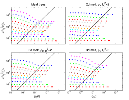
Figure 2: Parametric plots of the MC-time (t𝑡t) evolution of the ensemble-average square gyration radius, Rg2(t)delimited-⟨⟩superscriptsubscript𝑅𝑔2𝑡\langle R_{g}^{2}(t)\rangle, vs. the mean-square displacement of the tree center of mass, g3(t)subscript𝑔3𝑡g_{3}(t). Non-equilibrated (resp., equilibrated) values of the plots correspond to regions above (resp., below) the black solid line y=x𝑦𝑥y=x. Different colors correspond to different tree masses ranging from (bottom symbols) N=3𝑁3N=3 to (top symbols) N=900𝑁900N=900 (melts for ρKlK3=2subscript𝜌𝐾superscriptsubscript𝑙𝐾32\rho_{K}l_{K}^{3}=2) and N=1800𝑁1800N=1800 (ideal trees and melts for ρKlK3=5subscript𝜌𝐾superscriptsubscript𝑙𝐾35\rho_{K}l_{K}^{3}=5)

.

Amoeba trial moves simultaneously modify the tree connectivity, 𝒢𝒢{\mathcal{G}}, and the tree conformation, ΓΓ\Gamma. They are constructed by randomly cutting a leaf (or node with functionality f=1𝑓1f=1) from the tree and placing it on a randomly chosen site adjacent to a randomly chosen node with functionality f<3𝑓3f<3, to which the leave is then connected. Trial moves, 𝒯i𝒯fsubscript𝒯𝑖subscript𝒯𝑓{\cal T}_{i}\rightarrow{\cal T}_{f}, are accepted with probability:

accif=min{1,n1(i)n1(f)eβ((𝒯f)(𝒯i))}subscriptacc𝑖𝑓1subscript𝑛1𝑖subscript𝑛1𝑓superscript𝑒𝛽subscript𝒯𝑓subscript𝒯𝑖\mbox{acc}_{i\rightarrow f}=\min\left\{1,\frac{n_{1}(i)}{n_{1}(f)}e^{-\beta\left({\mathcal{H}}({\cal T}_{f})-{\mathcal{H}}({\cal T}_{i})\right)}\right\} (22)

where n1(i/f)subscript𝑛1𝑖𝑓n_{1}(i/f) is the total number of 1-functional nodes in the initial/final state and (𝒯)=id(𝒯)+int(𝒯)𝒯subscript𝑖𝑑𝒯subscript𝑖𝑛𝑡𝒯{\mathcal{H}}({\cal T})={\mathcal{H}}_{id}({\cal T})+{\mathcal{H}}_{int}({\cal T}), Eqs. (6) and (7). It should be noted, that our version of the amoeba algorithm is slightly modified with respect to the original one of Ref. SeitzKlein1981 as we impose RosaEveraersPRL2014 node functionalities f3𝑓3f\leq 3. Similar algorithms displacing entire branches are more efficient for single trees MadrasJPhysA1992 , but are likely to encounter difficulties when generalized to the dense systems we are mostly interested in. In contrast, the small non-local mass transport of the amoeba algorithm is not obstructed by the volume interactions, since it falls into the range of the natural occupancy fluctuations in our tree melts.

Our simulations start from linearly connected random walks as initial states. The total computational effort for equilibrating the systems as a function of the corresponding systems sizes is summarised in Table SI SupplMatNote . As illustrated by Fig. 2, the tree gyration radii equilibrate over a time scale during which the tree centers of mass diffuse over the corresponding distance. Quite curiously, the performance of the “amoeba” algorithm as a function of the Monte Carlo time steps is non-monotonic in the system density ρKsubscript𝜌𝐾\rho_{K}, see Fig. S1 SupplMatNote . In fact, while 3d3𝑑3d self-avoiding trees (ρKlK30subscript𝜌𝐾superscriptsubscript𝑙𝐾30\rho_{K}l_{K}^{3}\rightarrow 0, studied in our previous work Rosa2016a ) and 3d3𝑑3d melts for ρKlK3=5subscript𝜌𝐾superscriptsubscript𝑙𝐾35\rho_{K}l_{K}^{3}=5 take roughly the same time to reach equilibrium, 2d2𝑑2d and 3d3𝑑3d tree melts at density ρKlKd=2subscript𝜌𝐾superscriptsubscript𝑙𝐾𝑑2\rho_{K}l_{K}^{d}=2 require simulations which are 10absent10\approx 10 times longer. In particular, this is the reason why we have only been able to reach tree weights up to Nmax=900subscript𝑁max900N_{\mathrm{max}}=900 compared to Nmax=1800subscript𝑁max1800N_{\mathrm{max}}=1800 in Ref. RosaEveraersPRL2014 . At the moment we have no explanation accounting for this, apparently counterintuitive, behavior.

III.2 Analysis of tree connectivity

As in our previous work Rosa2016a , we have analysed tree connectivities using a variant of the “burning” algorithm for percolation clusters StanleyJPhysA1984 ; StaufferAharonyBook . The algorithm is very simple, and consists of two parts. In the initial inward (or burning) pass branch tips are iteratively “burned” until the tree center is reached. In the subsequent outward pass one advances from the center towards the periphery. The inward pass provides information about the mass and shape of branches. The outward pass allows to reconstruct the distance of nodes from the tree center. By employing a data structure in the form of a linked list, which retains for each node, i𝑖i, its position, risubscript𝑟𝑖\vec{r}_{i}, functionality, fisubscript𝑓𝑖f_{i}, and the indices {j1(i),,jfi(i)}subscript𝑗1𝑖subscript𝑗subscript𝑓𝑖𝑖\{j_{1}(i),\ldots,j_{f_{i}}(i)\} of the nodes to which it is connected, each step of the burning algorithm consists in removing from the list all sites with functionality =1absent1=1 (tips) and updating the functionalities and the indices of the remaining nodes accordingly. The algorithm stops when only one node remains in the list. In order to find the minimal path length l𝑙l between any pair of tree nodes i𝑖i and j𝑗j, we have modified the algorithm by requiring that sites i𝑖i and j𝑗j are not removed from the list. Accordingly, the algorithm stops when nodes i𝑖i and j𝑗j are the only tips left of the “burned” tree. By using the remaining linked list it is then trivial to find the corresponding path length l𝑙l.

III.3 Extracting exponents from data for finite-size trees

In order to get reliable estimates of critical exponents “ρ,ϵ,νpath,ν𝜌italic-ϵsubscript𝜈path𝜈\rho,\epsilon,\nu_{\mathrm{path}},\nu” in the large-N𝑁N limit and of the corresponding errors, we stay close to the procedure developed by Janse van Rensburg and Madras MadrasJPhysA1992 and employed in our previous work Rosa2016a , and combine the results obtained from fitting the N𝑁N-dependent data to two functional forms. For the specific example of the exponent ν𝜈\nu, they are given by the following expressions:

  1. 1.

    A simple power-law behavior with 222 (a𝑎a, ν𝜈\nu) fit parameters:

    logRg2(N)=a+2νlogN,superscriptsubscript𝑅𝑔2𝑁𝑎2𝜈𝑁\log\langle R_{g}^{2}(N)\rangle=a+2\nu\log N\,, (23)

    and

  2. 2.

    A power-law behavior with a correction-to-scaling term (NΔ0similar-toabsentsuperscript𝑁subscriptΔ0\sim N^{-\Delta_{0}}) with 444 (a𝑎a, b𝑏b, ΔΔ\Delta, ν𝜈\nu) fit parameters:

    logRg2(N)=superscriptsubscript𝑅𝑔2𝑁absent\displaystyle\log\langle R_{g}^{2}(N)\rangle=
    a+bNΔ0+2νlogNb(ΔΔ0)NΔ0logN.𝑎𝑏superscript𝑁subscriptΔ02𝜈𝑁𝑏ΔsubscriptΔ0superscript𝑁subscriptΔ0𝑁\displaystyle a+bN^{-\Delta_{0}}+2\nu\log N-b(\Delta-\Delta_{0})N^{-\Delta_{0}}\log N\,.

    Here, we have carried out a one-dimensional search for the value of Δ0subscriptΔ0\Delta_{0} for which the fit yields a vanishing NΔ0logNsuperscript𝑁subscriptΔ0𝑁N^{-\Delta_{0}}\log N term.

For the other exponents, we have employed analogous expressions. Eq. (23) has been used on data with N230𝑁230N\geq 230 and N450𝑁450N\geq 450 for ρKlKd=2subscript𝜌𝐾superscriptsubscript𝑙𝐾𝑑2\rho_{K}l_{K}^{d}=2 (d=2,3𝑑23d=2,3) and ρKlK3=5subscript𝜌𝐾superscriptsubscript𝑙𝐾35\rho_{K}l_{K}^{3}=5, respectively. Eq. (2) has been employed on the whole range with N10𝑁10N\geq 10. Best fits are obtained by minimizing NumericalRecipes χ2=i=1D[logRg2(Ni)observedlogRg2(Ni)modelδlogRg2(Ni)]2\chi^{2}=\sum_{i=1}^{D}\left[\frac{\log\langle R_{g}^{2}(N_{i})\rangle_{observed}-\log\langle R_{g}^{2}(N_{i})\rangle_{model}}{\delta\log\langle R_{g}^{2}(N_{i})\rangle}\right]^{2}, where D𝐷D is the number of data points used in the fit procedure. Quality of the fit is estimated by the normalized χ~2χ2Dfsuperscript~𝜒2superscript𝜒2𝐷𝑓{\tilde{\chi}}^{2}\equiv\frac{\chi^{2}}{D-f}, where f𝑓f is the number of fit parameters. When χ~21superscript~𝜒21{\tilde{\chi}}^{2}\approx 1 the fit is deemed to be reliable NumericalRecipes . The corresponding 𝒬(Df,χ2)𝒬𝐷𝑓superscript𝜒2\mathcal{Q}(D-f,\chi^{2})-values provide a quantitative indicator for the likelihood that χ2superscript𝜒2\chi^{2} should exceed the observed value, if the model were correct NumericalRecipes . All fit results are reported together with the corresponding errors, χ~2superscript~𝜒2{\tilde{\chi}}^{2} and 𝒬𝒬\mathcal{Q} values. Final estimates of critical exponents are calculated as averages of all independent measurements. Corresponding uncertainties are given in the form ±plus-or-minus\pm(statistical error)±plus-or-minus\pm(systematic error), where the “statistical error” is the largest value obtained from the different fits MadrasJPhysA1992 while the “systematic error” is the spread between the single estimates, respectively. In those cases where Eq. (2) fails producing trustable results we have retained only the 222-parameter fit, Eq. (23), and a separate analysis of uncertainties was required, see the caption of Table SVII SupplMatNote for details. Error bars reported in Table 1 are given by (statistical error)2+(systematic error)2superscriptstatistical error2superscriptsystematic error2\sqrt{(\mbox{statistical error})^{2}+(\mbox{systematic error})^{2}}.

IV Results

In the following sections, we discuss the structure of trees in 2d2𝑑2d and 3d3𝑑3d melts by considering the scaling behaviors of the observables defined in Sec. II.2 and their corresponding critical exponents. Similarly to the general outline of our previous work Rosa2016a on single self-avoiding trees in good solvent, it is particularly instructive to compare the properties of interacting trees to the ones for ideal trees. For this reason, but also for keeping this work autonomous and self-consistent in its own, all figures and tables of this work, including the supplementary ones SupplMatNote , contain the same data for ideal trees originally reported in Rosa2016a .

IV.1 Branching statistics for trees with annealed connectivity
Refer to caption
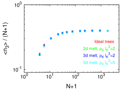
Figure 3: Branching statistics. Average fraction of 333-functional nodes, n3N+1delimited-⟨⟩subscript𝑛3𝑁1\frac{\langle n_{3}\rangle}{N+1}, as a function of the total number of tree nodes, N+1𝑁1N+1. The asymptotic branching probability Rosa2016a λ𝜆\lambda is =0.4absent0.4=0.4.

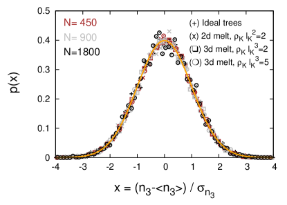
Our results for the average number of branch points, n3(N)delimited-⟨⟩subscript𝑛3𝑁\langle n_{3}(N)\rangle, as a function of N𝑁N are listed in Tables SII-III SupplMatNote . Figure 3 shows that the ratios of 3-functional nodes, n3(N)/Ndelimited-⟨⟩subscript𝑛3𝑁𝑁\langle n_{3}(N)\rangle/N, reach their asymptotic value already for moderate tree weights. Interestingly, our results for ideal trees as well as interacting trees perfectly agree to each other with asymptotic branching probability Rosa2016a λ=limNn3(N)/N=0.4𝜆subscript𝑁delimited-⟨⟩subscript𝑛3𝑁𝑁0.4\lambda=\lim_{N\rightarrow\infty}\langle n_{3}(N)\rangle/N=0.4. In fact, due to the multiple occupation of lattice sites in the melt, the branching probabilities remain virtually unchanged in spite of the interactions. Corresponding distributions p(n3)𝑝subscript𝑛3p(n_{3}) are well described by Gaussian statistics with corresponding variances increasing linearly with N𝑁N, see Fig. S2 SupplMatNote .

IV.2 Path length statistics for trees
Refer to caption
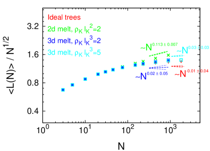
Figure 4: Path length statistics. Mean contour distance between pairs of nodes, L(N)delimited-⟨⟩𝐿𝑁\langle L(N)\rangle. Straight lines correspond to the large-N𝑁N behaviour L(N)Nρsimilar-todelimited-⟨⟩𝐿𝑁superscript𝑁𝜌\langle L(N)\rangle\sim N^{\rho} with critical exponents ρ𝜌\rho given by the best estimates summarised in Table 1.

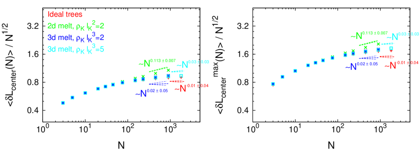
Our results for (A) the mean contour distance between pairs of nodes, L(N)delimited-⟨⟩𝐿𝑁\langle L(N)\rangle, (B) the mean contour distance of nodes from the central node, δLcenter(N)delimited-⟨⟩𝛿subscript𝐿center𝑁\langle\delta L_{\mathrm{center}}(N)\rangle, and (C) the mean longest contour distance of nodes from the central node, δLcentermax(N)delimited-⟨⟩𝛿superscriptsubscript𝐿centermax𝑁\langle\delta L_{\mathrm{center}}^{\mathrm{max}}(N)\rangle are summarized in Tables SII-III SupplMatNote and plotted in Fig. 4 and Fig. S3 SupplMatNote . As discussed in Sec. II.2, the three quantities are expected to scale with the total tree weight N𝑁N as δLcenter(N)δLcentermax(N)L(N)Nρsimilar-todelimited-⟨⟩𝛿subscript𝐿center𝑁delimited-⟨⟩𝛿superscriptsubscript𝐿centermax𝑁similar-todelimited-⟨⟩𝐿𝑁similar-tosuperscript𝑁𝜌\langle\delta L_{\mathrm{center}}(N)\rangle\sim\langle\delta L_{\mathrm{center}}^{\mathrm{max}}(N)\rangle\sim\langle L(N)\rangle\sim N^{\rho}. Extracted single values for ρ𝜌\rho’s including more details on their statistical significance (χ2superscript𝜒2\chi^{2} and 𝒬𝒬\mathcal{Q}-values) are summarized in Table SIV SupplMatNote . Our final best estimates for ρ𝜌\rho’s (straight lines in Fig. 4 and Fig. S3 SupplMatNote , and Tables 1 and SIV SupplMatNote ) are obtained by combining the corresponding results for δLcenter(N)delimited-⟨⟩𝛿subscript𝐿center𝑁\langle\delta L_{\mathrm{center}}(N)\rangle, δLcentermax(N)delimited-⟨⟩𝛿superscriptsubscript𝐿centermax𝑁\langle\delta L_{\mathrm{center}}^{\mathrm{max}}(N)\rangle and L(N)delimited-⟨⟩𝐿𝑁\langle L(N)\rangle.

IV.3 Path lengths vs. weights for branches
Refer to caption
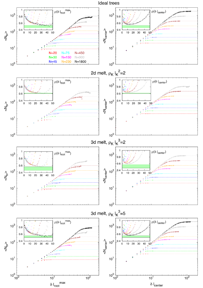
Figure 5: Path lengths vs. weights of branches. Data for trees of weight from N=20𝑁20N=20 to N=1800𝑁1800N=1800. (Left) Average branch weight, Nbr(δlrootmax)delimited-⟨⟩subscript𝑁𝑏𝑟𝛿superscriptsubscript𝑙rootmax\langle N_{br}(\delta l_{\mathrm{root}}^{\mathrm{max}})\rangle, as a function of the longest contour distance to the branch root, δlrootmax𝛿superscriptsubscript𝑙rootmax\delta l_{\mathrm{root}}^{\mathrm{max}}. For large δlrootmax𝛿superscriptsubscript𝑙rootmax\delta l_{\mathrm{root}}^{\mathrm{max}}, curves saturate to the corresponding maximal branch weight (N1)/2𝑁12(N-1)/2 (dashed horizontal lines). (Right) Average branch weight, Ncenter(δlcenter)delimited-⟨⟩subscript𝑁𝑐𝑒𝑛𝑡𝑒𝑟𝛿subscript𝑙center\langle N_{center}(\delta l_{\mathrm{center}})\rangle, composed of segments whose distance from the central node does not exceed δLcenter𝛿subscript𝐿center\delta L_{\mathrm{center}}. For large δlcenter𝛿subscript𝑙center\delta l_{\mathrm{center}}, curves saturate to the corresponding total tree weight, N𝑁N (dashed horizontal lines). Insets: Corresponding differential fractal exponent ρ(δlrootmax)𝜌𝛿superscriptsubscript𝑙rootmax\rho(\delta l_{\mathrm{root}}^{\mathrm{max}}) and ρ(δlcenter)𝜌𝛿subscript𝑙center\rho(\delta l_{\mathrm{center}}). Shaded regions show the range of ρ𝜌\rho values summarized in Table 1.

The relation between branch weight and path length can also be explored on the level of branches. We have analyzed the scaling behavior of: (1) the average branch weight, Nbr(δlrootmax)delimited-⟨⟩subscript𝑁𝑏𝑟𝛿superscriptsubscript𝑙rootmax\langle N_{br}(\delta l_{\mathrm{root}}^{\mathrm{max}})\rangle, as a function of the longest contour distance to the branch root, δlrootmax𝛿superscriptsubscript𝑙rootmax\delta l_{\mathrm{root}}^{\mathrm{max}}, and (2) the average branch (or tree core) weight, Ncenter(δlcenter)delimited-⟨⟩subscript𝑁center𝛿subscript𝑙center\langle N_{\mathrm{center}}(\delta l_{\mathrm{center}})\rangle, inside a contour distance δlcenter𝛿subscript𝑙center\delta l_{\mathrm{center}} from the central node of the tree. Corresponding results are shown in Fig. 5. Both data sets show universal behavior at intermediate δlrootmax𝛿superscriptsubscript𝑙rootmax\delta l_{\mathrm{root}}^{\mathrm{max}} and δlcenter𝛿subscript𝑙center\delta l_{\mathrm{center}}, and saturate to the corresponding expected limiting values =N12absent𝑁12=\frac{N-1}{2} and =Nabsent𝑁=N. For large δlrootmax𝛿superscriptsubscript𝑙rootmax\delta l_{\mathrm{root}}^{\mathrm{max}} (respectively, δlcenter𝛿subscript𝑙center\delta l_{\mathrm{center}}) the relation Nbr(δlrootmax)δlrootmax1/ρsimilar-todelimited-⟨⟩subscript𝑁𝑏𝑟𝛿superscriptsubscript𝑙rootmax𝛿superscriptsuperscriptsubscript𝑙rootmax1𝜌\langle N_{br}(\delta l_{\mathrm{root}}^{\mathrm{max}})\rangle\sim{\delta l_{\mathrm{root}}^{\mathrm{max}}}^{1/\rho} (resp., Ncenter(δlcenter)δlcenter1/ρsimilar-todelimited-⟨⟩subscript𝑁center𝛿subscript𝑙center𝛿superscriptsubscript𝑙center1𝜌\langle N_{\mathrm{center}}(\delta l_{\mathrm{center}})\rangle\sim{\delta l_{\mathrm{center}}}^{1/\rho}) is expected to hold. For Nbrsubscript𝑁𝑏𝑟N_{br} (and with an analogous expression for Ncenter)N_{center}), we have estimated ρ𝜌\rho as ρ(δlrootmax)=(logNbr(δlrootmax+1)/Nbr(δlrootmax)log(δlrootmax+1)/δlrootmax)1𝜌𝛿superscriptsubscript𝑙rootmaxsuperscriptsubscript𝑁𝑏𝑟𝛿superscriptsubscript𝑙rootmax1delimited-⟨⟩subscript𝑁𝑏𝑟𝛿superscriptsubscript𝑙rootmax𝛿superscriptsubscript𝑙rootmax1𝛿superscriptsubscript𝑙rootmax1\rho(\delta l_{\mathrm{root}}^{\mathrm{max}})=\left(\frac{\log\,\langle N_{br}(\delta l_{\mathrm{root}}^{\mathrm{max}}+1)\rangle/\langle N_{br}(\delta l_{\mathrm{root}}^{\mathrm{max}})\rangle}{\log\,(\delta l_{\mathrm{root}}^{\mathrm{max}}+1)/\delta l_{\mathrm{root}}^{\mathrm{max}}}\right)^{-1}. Numerical results are reported in the corresponding insets of Fig. 5, the large-scale behaviour agreeing well with the best estimates for ρ𝜌\rho’s (horizontal lines) summarized in Table 1.

IV.4 Branch weight statistics
Refer to caption
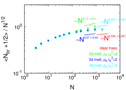
Figure 6: Branch weight statistics. Average branch weight, Nbr(N)delimited-⟨⟩subscript𝑁𝑏𝑟𝑁\langle N_{br}(N)\rangle as a function of the total tree mass, N𝑁N. Straight lines correspond to the large-N𝑁N behaviour Nbr(N)Nϵsimilar-todelimited-⟨⟩subscript𝑁𝑏𝑟𝑁superscript𝑁italic-ϵ\langle N_{br}(N)\rangle\sim N^{\epsilon} with critical exponents ϵitalic-ϵ\epsilon given by the best estimates summarised in Table 1.

The scaling behavior of the average branch weight, Nbr(N)Nϵsimilar-todelimited-⟨⟩subscript𝑁𝑏𝑟𝑁superscript𝑁italic-ϵ\langle N_{br}(N)\rangle\sim N^{\epsilon}, defines the critical exponent ϵitalic-ϵ\epsilon. Single values of Nbr(N)delimited-⟨⟩subscript𝑁𝑏𝑟𝑁\langle N_{br}(N)\rangle for each N𝑁N (see Tables SII-III SupplMatNote ) are plotted in Fig. 6, where the straight lines have slopes corresponding to our best estimates for ϵitalic-ϵ\epsilon’s (Table 1), see also Table SIV SupplMatNote for details. We notice, in particular, that the scaling relation ρ=ϵ𝜌italic-ϵ\rho=\epsilon holds within error bars.

IV.5 Conformational statistics of linear paths
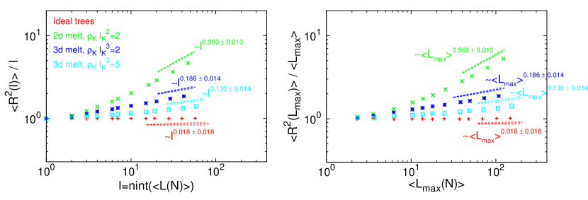
Refer to caption
Figure 7: Conformational statistics of linear paths. (Left) Mean-square end-to-end distance, R2(=𝚗𝚒𝚗𝚝(L))delimited-⟨⟩superscript𝑅2𝚗𝚒𝚗𝚝delimited-⟨⟩𝐿\langle R^{2}(\ell={\tt nint}(\langle L\rangle))\rangle, of paths of length =𝚗𝚒𝚗𝚝(L(N))𝚗𝚒𝚗𝚝delimited-⟨⟩𝐿𝑁absent\ell={\tt nint}(\langle L(N)\rangle)\equiv closest-integer-to L(N)delimited-⟨⟩𝐿𝑁\langle L(N)\rangle. (Right) Mean-square end-to-end distance, R2(Lmax)delimited-⟨⟩superscript𝑅2subscript𝐿max\langle R^{2}(L_{\mathrm{max}})\rangle, of the longest paths. Straight lines correspond to the large-\ell or large-Lmax(N)delimited-⟨⟩subscript𝐿max𝑁\langle L_{\mathrm{max}}(N)\rangle behaviours: R2()2νpathsimilar-todelimited-⟨⟩superscript𝑅2superscript2subscript𝜈path\langle R^{2}(\ell)\rangle\sim\ell^{2\nu_{\mathrm{path}}} or R2(Lmax)Lmax(N)2νpathsimilar-todelimited-⟨⟩superscript𝑅2subscript𝐿maxsuperscriptdelimited-⟨⟩subscript𝐿max𝑁2subscript𝜈path\langle R^{2}(L_{\mathrm{max}})\rangle\sim\langle L_{\mathrm{max}}(N)\rangle^{2\nu_{\mathrm{path}}}. Critical exponents νpathsubscript𝜈path\nu_{\mathrm{path}} are given by the best estimates reported in Table 1.

In order to extract the critical exponent νpathsubscript𝜈path\nu_{\mathrm{path}} which defines the scaling behavior R2(l,N)l2νpathsimilar-todelimited-⟨⟩superscript𝑅2𝑙𝑁superscript𝑙2subscript𝜈path\langle R^{2}(l,N)\rangle\sim l^{2\nu_{\mathrm{path}}}, we have selected paths of length close to the average length (l=L(N)𝑙delimited-⟨⟩𝐿𝑁l=\langle L(N)\rangle) and to the trees maximal length (l=Lmax(N)𝑙subscript𝐿max𝑁l=L_{\mathrm{max}}(N)) and calculated corresponding mean-square end-to-end distances R2(L)L(N)2νpathsimilar-todelimited-⟨⟩superscript𝑅2delimited-⟨⟩𝐿superscriptdelimited-⟨⟩𝐿𝑁2subscript𝜈path\langle R^{2}(\langle L\rangle)\rangle\sim\langle L(N)\rangle^{2\nu_{\mathrm{path}}} and R2(Lmax)Lmax(N)2νpathsimilar-todelimited-⟨⟩superscript𝑅2subscript𝐿maxsuperscriptdelimited-⟨⟩subscript𝐿max𝑁2subscript𝜈path\langle R^{2}(L_{\mathrm{max}})\rangle\sim\langle L_{\mathrm{max}}(N)\rangle^{2\nu_{\mathrm{path}}} (see Fig. 7 and corresponding tabulated values in Tables SV-VI SupplMatNote . Combination of the two (Table SVII SupplMatNote ) led to our best estimates for νpathsubscript𝜈path\nu_{\mathrm{path}} in the different ensembles summarized in Table 1. Not surprisingly, these values agree well with the differential exponents νpath(l)=12logR2(l+1,N)/R2(l,N)log(l+1)/lsubscript𝜈path𝑙12superscript𝑅2𝑙1𝑁delimited-⟨⟩superscript𝑅2𝑙𝑁𝑙1𝑙\nu_{\mathrm{path}}(l)=\frac{1}{2}\frac{\log\,\langle R^{2}(l+1,N)\rangle/\langle R^{2}(l,N)\rangle}{\log\,(l+1)/l} reported in the l.h.s insets of Fig. 8.
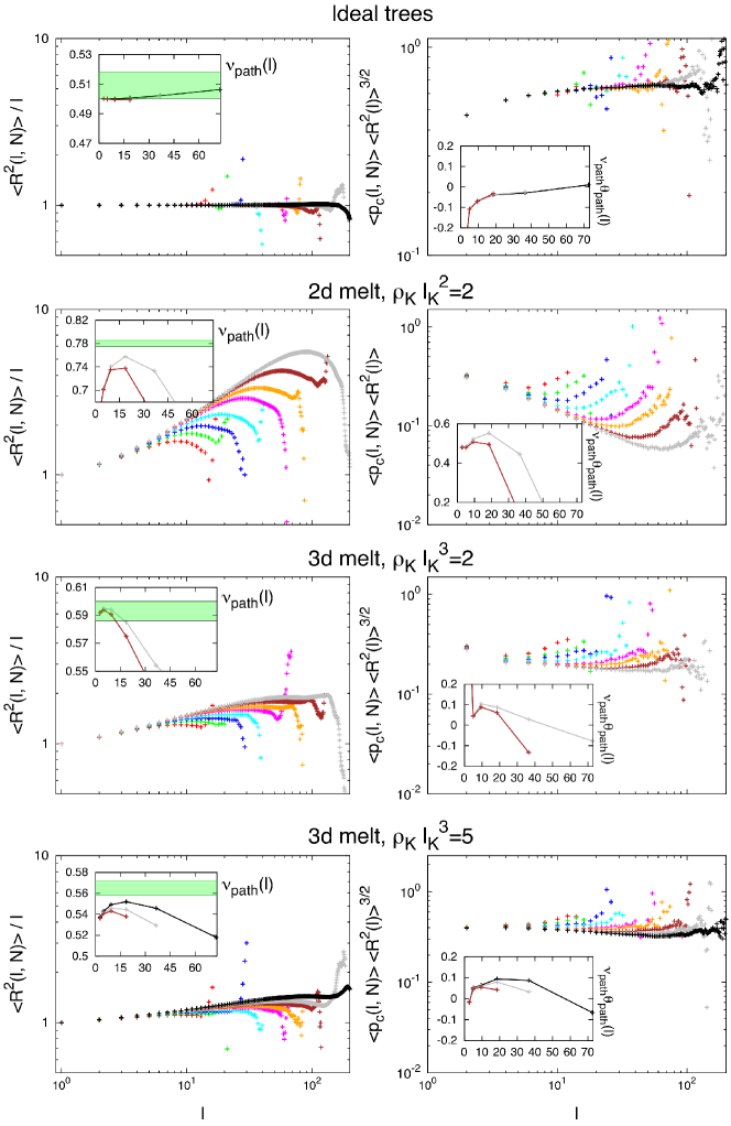
Refer to caption
Figure 8: Conformational statistics of linear paths. (L.h. column) Mean-square end-to-end distance, R2(l,N)delimited-⟨⟩superscript𝑅2𝑙𝑁\langle R^{2}(l,N)\rangle, of linear paths of length l𝑙l. Insets: Differential fractal exponent, νpath(l)=12logR2(l+1,N)/R2(l,N)log(l+1)/lsubscript𝜈path𝑙12superscript𝑅2𝑙1𝑁delimited-⟨⟩superscript𝑅2𝑙𝑁𝑙1𝑙\nu_{\mathrm{path}}(l)=\frac{1}{2}\frac{\log\,\langle R^{2}(l+1,N)\rangle/\langle R^{2}(l,N)\rangle}{\log\,(l+1)/l} for chain lengths N450𝑁450N\geq 450. Shaded regions show the range of νpathsubscript𝜈path\nu_{\mathrm{path}} values summarized in Table 1. (R.h. column) Mean closure probabilities, pc(l,N)delimited-⟨⟩subscript𝑝𝑐𝑙𝑁\langle p_{c}(l,N)\rangle, between ends of linear paths of length l𝑙l normalised to the mean-field expectation value R2(l,N)3/2superscriptdelimited-⟨⟩superscript𝑅2𝑙𝑁32\langle R^{2}(l,N)\rangle^{-3/2}. Insets: Differential fractal exponent νpathθpath(l)subscript𝜈pathsubscript𝜃path𝑙\nu_{\mathrm{path}}\theta_{\mathrm{path}}(l), see Eq. (5), defined analogously to νpath(l)subscript𝜈path𝑙\nu_{\mathrm{path}}(l) for chain lengths N450𝑁450N\geq 450. Plots in the insets have been obtained by averaging corresponding quantities over log-spaced intervals. Color code is as in Fig. 5.

Then, we have calculated the mean closure probabilities, pc(l,N)delimited-⟨⟩subscript𝑝𝑐𝑙𝑁\langle p_{c}(l,N)\rangle (Fig. 8, right-hand panels), normalised to the corresponding “mean-field” expectation values R2(l,N)3/2l3νpathsimilar-tosuperscriptdelimited-⟨⟩superscript𝑅2𝑙𝑁32superscript𝑙3subscript𝜈path\langle R^{2}(l,N)\rangle^{-3/2}\sim l^{-3\nu_{\mathrm{path}}}. As in the case of single self-avoiding trees in good solvent Rosa2016a , pc(l,N)delimited-⟨⟩subscript𝑝𝑐𝑙𝑁\langle p_{c}(l,N)\rangle for interacting trees markedly deviate from the mean-field prediction, which defines a novel critical exponent θpathsubscript𝜃path\theta_{\mathrm{path}}, pc(l,N)R2(l,N)3/2lνpathθpathsimilar-todelimited-⟨⟩subscript𝑝𝑐𝑙𝑁superscriptdelimited-⟨⟩superscript𝑅2𝑙𝑁32superscript𝑙subscript𝜈pathsubscript𝜃path\langle p_{c}(l,N)\rangle\langle R^{2}(l,N)\rangle^{3/2}\sim l^{-\nu_{\mathrm{path}}\theta_{\mathrm{path}}}. Estimated values for θpathsubscript𝜃path\theta_{\mathrm{path}}’s are reported in Table 1.

IV.6 Conformational statistics of trees
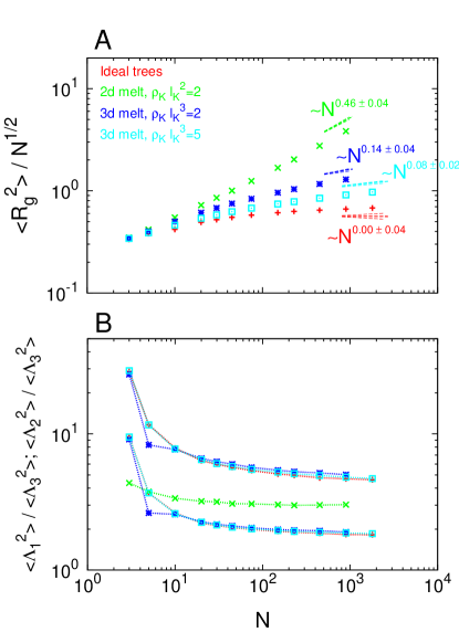
Refer to caption
Figure 9: Conformational statistics of trees. (A) Mean square gyration radius, Rg2(N)delimited-⟨⟩superscriptsubscript𝑅𝑔2𝑁\langle R_{g}^{2}(N)\rangle. Straight lines correspond to the large-N𝑁N behaviour Rg2(N)N2νsimilar-todelimited-⟨⟩superscriptsubscript𝑅𝑔2𝑁superscript𝑁2𝜈\langle R_{g}^{2}(N)\rangle\sim N^{2\nu} with critical exponents ν𝜈\nu given by the best estimates summarised in Table 1. (B) Tree average aspect ratios, Λ12/Λ32delimited-⟨⟩superscriptsubscriptΛ12delimited-⟨⟩superscriptsubscriptΛ32\langle\Lambda_{1}^{2}\rangle/\langle\Lambda_{3}^{2}\rangle and Λ22/Λ32delimited-⟨⟩superscriptsubscriptΛ22delimited-⟨⟩superscriptsubscriptΛ32\langle\Lambda_{2}^{2}\rangle/\langle\Lambda_{3}^{2}\rangle.

Finally, we have measured the mean-square gyration radius, Rg2(N)delimited-⟨⟩superscriptsubscript𝑅𝑔2𝑁\langle R_{g}^{2}(N)\rangle (tabulated values in Tables SV-VI SupplMatNote ), and the average shape of trees as a function of tree weight, N𝑁N (Fig. 9, panels A and B respectively). Estimated values of critical exponents ν𝜈\nu (straight lines in Fig. 9A) are summarized in Table 1, while details about their derivation are given in Table SVII SupplMatNote .

V Discussion

Ideal trees with 2d2𝑑2d melt of trees with 3d3𝑑3d melt of trees with 3d3𝑑3d melt of trees with
annealed connectivity annealed connectivity annealed connectivity annealed connectivity
Relation to Theory Simul. Theory Simul., ρKlK2=2subscript𝜌𝐾superscriptsubscript𝑙𝐾22\rho_{K}l_{K}^{2}=2 Theory Simul., ρKlK3=2subscript𝜌𝐾superscriptsubscript𝑙𝐾32\rho_{K}l_{K}^{3}=2 Simul., ρKlK3=5subscript𝜌𝐾superscriptsubscript𝑙𝐾35\rho_{K}l_{K}^{3}=5
other exponents
ρ𝜌\rho 12=0.5120.5\frac{1}{2}=0.5 0.49±0.04plus-or-minus0.490.040.49\pm 0.04 230.667230.667\frac{2}{3}\approx 0.667 0.613±0.007plus-or-minus0.6130.0070.613\pm 0.007 590.556590.556\frac{5}{9}\approx 0.556 0.52±0.05plus-or-minus0.520.050.52\pm 0.05 0.53±0.03plus-or-minus0.530.030.53\pm 0.03
ϵitalic-ϵ\epsilon =ρabsent𝜌=\rho 12=0.5120.5\frac{1}{2}=0.5 0.536±0.007plus-or-minus0.5360.0070.536\pm 0.007 230.667230.667\frac{2}{3}\approx 0.667 0.63±0.01plus-or-minus0.630.010.63\pm 0.01 590.556590.556\frac{5}{9}\approx 0.556 0.57±0.02plus-or-minus0.570.020.57\pm 0.02 0.554±0.006plus-or-minus0.5540.0060.554\pm 0.006
νpathsubscript𝜈path\nu_{\mathrm{path}} 12=0.5120.5\frac{1}{2}=0.5 0.509±0.009plus-or-minus0.5090.0090.509\pm 0.009 34=0.75340.75\frac{3}{4}=0.75 0.780±0.005plus-or-minus0.7800.0050.780\pm 0.005 35=0.6350.6\frac{3}{5}=0.6 0.593±0.007plus-or-minus0.5930.0070.593\pm 0.007 0.565±0.007plus-or-minus0.5650.0070.565\pm 0.007
ν𝜈\nu =ρνpathabsent𝜌subscript𝜈path=\rho\,\nu_{\mathrm{path}} 14=0.25140.25\frac{1}{4}=0.25 0.25±0.02plus-or-minus0.250.020.25\pm 0.02 12=0.5120.5\frac{1}{2}=0.5 0.48±0.02plus-or-minus0.480.020.48\pm 0.02 130.333130.333\frac{1}{3}\approx 0.333 0.32±0.02plus-or-minus0.320.020.32\pm 0.02 0.29±0.01plus-or-minus0.290.010.29\pm 0.01
θpathsubscript𝜃path\theta_{\mathrm{path}} 0.04±0.04plus-or-minus0.040.04-0.04\pm 0.04 0.65±0.06plus-or-minus0.650.060.65\pm 0.06 0.12±0.05plus-or-minus0.120.050.12\pm 0.05 0.14±0.02plus-or-minus0.140.020.14\pm 0.02
Table 1: Asymptotic (left) and crossover (right) critical exponents for 2d2𝑑2d and 3d3𝑑3d lattice trees. (a) ρ𝜌\rho, ϵitalic-ϵ\epsilon, νpathsubscript𝜈path\nu_{\mathrm{path}} and ν𝜈\nu: Comparison between predictions of Flory theory and numerical results. As explained in Sec. III.3, numerical results for ρ𝜌\rho, ϵitalic-ϵ\epsilon and ν𝜈\nu (for this last exponent, with the only exception of 2d2𝑑2d melts) were derived by combining values and statistical errors of the parameters obtained from best fits (Tables SIV and SVII SupplMatNote ) of Eqs. (23) and (2) to corresponding observables. For νpathsubscript𝜈path\nu_{\mathrm{path}} and ν𝜈\nu in 2d2𝑑2d melts, Eq. (2) fails (Table SVII SupplMatNote ) and only Eq. (23) was employed. (b) θpathsubscript𝜃path\theta_{\mathrm{path}}: Numerical results are obtained by combining the estimated values of νpathsubscript𝜈path\nu_{\mathrm{path}} with the values of “νpathθpathsubscript𝜈pathsubscript𝜃path\nu_{\mathrm{path}}\theta_{\mathrm{path}}” averaged over the ranges of l𝑙l’s where this quantity shows a quasi-plateau for N=900𝑁900N=900 or N=1800𝑁1800N=1800 (see grey and black lines in the insets of the r.h.s panels of Fig. 8): νpathθpath=0.02±0.02subscript𝜈pathsubscript𝜃pathplus-or-minus0.020.02\nu_{\mathrm{path}}\theta_{\mathrm{path}}=-0.02\pm 0.02 (ideal trees); νpathθpath=0.51±0.05subscript𝜈pathsubscript𝜃pathplus-or-minus0.510.05\nu_{\mathrm{path}}\theta_{\mathrm{path}}=0.51\pm 0.05 (2d2𝑑2d melt of trees, ρKlK2=2subscript𝜌𝐾superscriptsubscript𝑙𝐾22\rho_{K}l_{K}^{2}=2); νpathθpath=0.07±0.03subscript𝜈pathsubscript𝜃pathplus-or-minus0.070.03\nu_{\mathrm{path}}\theta_{\mathrm{path}}=0.07\pm 0.03 (3d3𝑑3d melt of trees, ρKlK3=2subscript𝜌𝐾superscriptsubscript𝑙𝐾32\rho_{K}l_{K}^{3}=2); νpathθpath=0.08±0.01subscript𝜈pathsubscript𝜃pathplus-or-minus0.080.01\nu_{\mathrm{path}}\theta_{\mathrm{path}}=0.08\pm 0.01 (3d3𝑑3d melt of trees, ρKlK3=5subscript𝜌𝐾superscriptsubscript𝑙𝐾35\rho_{K}l_{K}^{3}=5). Average values and corresponding error bars have been rounded to the first significant decimal digit.

We have analyzed the behavior of interacting trees with annealed connectivity in 2d2𝑑2d and 3d3𝑑3d melts in terms of a small set of exponents defined in the Introduction and in Sec. II.2. With weights of up to N=1800𝑁1800N=1800 segments, our tree sizes are comparable to those of linear chains in similar studies MeyerWittmerJCP2010 ; WittmerReview2011 ; MeyerWittmerMacromolecules2012 . However, for many purposes the average contour distance, L𝒪(100)Ndelimited-⟨⟩𝐿𝒪100much-less-than𝑁\langle L\rangle\leq{\cal O}(100)\ll N, between monomers provides a more suitable comparison. The reader should thus bear in mind, that extracted exponents are either (i) effective (crossover) exponents valid for the particular systems and system sizes we have studied or (ii) estimates of true, asymptotic exponents, which suffer from uncertainties related to the extrapolation to the asymptotic limit. These effects are particularly pronounced for the high density 3d3𝑑3d melts we studied in Ref. RosaEveraersPRL2014 . For example, we initially reported RosaEveraersPRL2014 the results of a simple power law fit including all data for tree sizes N75𝑁75N\geq 75 suggesting ν=0.32±0.01𝜈plus-or-minus0.320.01\nu=0.32\pm 0.01. In contrast, the present more refined analysis yields ν=0.29±0.01𝜈plus-or-minus0.290.01\nu=0.29\pm 0.01. If this result is acceptable as an effective exponent for tree sizes N=𝒪(1000)𝑁𝒪1000N={\mathcal{O}}(1000), it mostly illustrates that one cannot extract the asymptotic behaviour assuming a single, small correction to scaling, if the available tree sizes barely reach the crossover (Sec. II.5). The discussion below focuses on results for lower density 2d2𝑑2d and 3d3𝑑3d melts, where the studied tree sizes are significantly larger than the estimated blob size.

Our results are summarised in Table 1. Most of them are in quantitative or at least good qualitative agreement with the predictions from Flory theory IsaacsonLubensky ; DaoudJoanny1981 ; GutinGrosberg93 ; GrosbergSoftMatter2014 . First, this implies that the reported exponents νpathsubscript𝜈path\nu_{\mathrm{path}} for melts of trees fit to the predicted GrosbergSoftMatter2014 value 3d+23𝑑2\frac{3}{d+2} which, intriguingly, corresponds to the Flory Flory1969 exponent ν𝜈\nu for self-avoiding linear chains in good solvent conditions. Second, the results for the exponent ν𝜈\nu are in agreement with the prediction ν=1/d𝜈1𝑑\nu=1/d and confirm that trees in melts behave as “territorial” polymers. This result is relatively simple to understand as ν=1/d𝜈1𝑑\nu=1/d represents the minimal amount of swelling compatible with steric packing requirements. Thus not too much stock should be put in the fact that the Flory value for ν𝜈\nu turns out to be exact in the present case. More interestingly, the theory makes two testable, non-trivial predictions for the contributions of connectivity changes and path stretching to the overall swelling GutinGrosberg93 (Eqs. (13) and (14)): firstly, both effects should only depend on the magnitude of the overall swelling, but not its physical origin and secondly path stretching is expected to be dominant as WeakStretchingNote νpathνpathideal2(ρρideal)=4(ννideal)/3subscript𝜈pathsuperscriptsubscript𝜈pathideal2𝜌superscript𝜌ideal4𝜈superscript𝜈ideal3\nu_{\mathrm{path}}-\nu_{\mathrm{path}}^{\mathrm{ideal}}\approx 2(\rho-\rho^{\mathrm{ideal}})=4(\nu-\nu^{\mathrm{ideal}})/3 for weakly swollen trees. The first prediction is well borne out by the comparison of 3d3𝑑3d self avoiding trees and 2d2𝑑2d melt trees. In both cases, the trees are expected to swell to ν=1/2𝜈12\nu=1/2. Interestingly, the observed values for ρ𝜌\rho and νpathsubscript𝜈path\nu_{\mathrm{path}} turn out to be almost identical and close to the predicted values. The second prediction is confirmed by noticing that trees in 2d2𝑑2d and 3d3𝑑3d melts swell almost exclusively at the path level (Fig. 7), while the observed modifications of the connectivities (Figs. 4 and 6), are very weak. In absolute terms for our largest trees with N=900𝑁900N=900 (see Tables SII-III SupplMatNote and SV-VI SupplMatNote ): Rg22dmelt/Rg2ideal=5.78±0.03subscriptdelimited-⟨⟩superscriptsubscript𝑅𝑔22𝑑meltsubscriptdelimited-⟨⟩superscriptsubscript𝑅𝑔2idealplus-or-minus5.780.03\langle R_{g}^{2}\rangle_{2d\ \mathrm{melt}}/\langle R_{g}^{2}\rangle_{\mathrm{ideal}}=5.78\pm 0.03, R2(Lmax)2dmelt/R2(Lmax)ideal=6.32±0.10subscriptdelimited-⟨⟩superscript𝑅2subscript𝐿max2𝑑meltsubscriptdelimited-⟨⟩superscript𝑅2subscript𝐿maxidealplus-or-minus6.320.10\langle R^{2}(L_{\mathrm{max}})\rangle_{2d\ \mathrm{melt}}/\langle R^{2}(L_{\mathrm{max}})\rangle_{\mathrm{ideal}}=6.32\pm 0.10 and L2dmelt/Lideal=1.188±0.002subscriptdelimited-⟨⟩𝐿2𝑑meltsubscriptdelimited-⟨⟩𝐿idealplus-or-minus1.1880.002\langle L\rangle_{2d\ \mathrm{melt}}/\langle L\rangle_{\mathrm{ideal}}=1.188\pm 0.002 while Rg23dmelt/Rg2ideal=1.95±0.02subscriptdelimited-⟨⟩superscriptsubscript𝑅𝑔23𝑑meltsubscriptdelimited-⟨⟩superscriptsubscript𝑅𝑔2idealplus-or-minus1.950.02\langle R_{g}^{2}\rangle_{3d\ \mathrm{melt}}/\langle R_{g}^{2}\rangle_{\mathrm{ideal}}=1.95\pm 0.02, R2(Lmax)3dmelt/R2(Lmax)ideal=1.96±0.03subscriptdelimited-⟨⟩superscript𝑅2subscript𝐿max3𝑑meltsubscriptdelimited-⟨⟩superscript𝑅2subscript𝐿maxidealplus-or-minus1.960.03\langle R^{2}(L_{\mathrm{max}})\rangle_{3d\ \mathrm{melt}}/\langle R^{2}(L_{\mathrm{max}})\rangle_{\mathrm{ideal}}=1.96\pm 0.03 and L3dmelt/Lideal=1.054±0.003subscriptdelimited-⟨⟩𝐿3𝑑meltsubscriptdelimited-⟨⟩𝐿idealplus-or-minus1.0540.003\langle L\rangle_{3d\ \mathrm{melt}}/\langle L\rangle_{\mathrm{ideal}}=1.054\pm 0.003.

For other quantities, Flory theory is even qualitatively wrong. A particularly interesting case are the average contact probability pc(l)delimited-⟨⟩subscript𝑝𝑐𝑙\langle p_{c}(l)\rangle between nodes at path distance l𝑙l. As shown in Fig. 8 and Table 1, pc(l)delimited-⟨⟩subscript𝑝𝑐𝑙\langle p_{c}(l)\rangle’s for interacting trees deviate consistently from the naïve mean-field estimate of l3νpathsuperscript𝑙3subscript𝜈pathl^{-3\nu_{\mathrm{path}}}. This is yet another illustration of the subtle cancellation of errors in Flory arguments, which are built on the mean-field estimates of contact probabilities DeGennesBook .

VI Summary and Conclusion

Motivated by the close analogy between non-concatenated ring polymers and annealed lattice trees KhokhlovNechaev85 ; RubinsteinPRL1986 ; RubinsteinPRL1994 ; RosaEveraersPRL2014 ; GrosbergSoftMatter2014 , we have studied the statistical properties of tree melts in d=2𝑑2d=2 and d=3𝑑3d=3 dimensions. We have used the same methodology as in our recent work on self-avoiding trees Rosa2016a , i.e. variants of the amoeba SeitzKlein1981 and burning StanleyJPhysA1984 ; StaufferAharonyBook algorithms for the Monte Carlo simulation and the connectivity analysis (Sec. III). Table 1 summarises our estimates of the asymptotic values of the exponents describing the scaling behavior of the average branch weight, Nbr(N)Nϵsimilar-todelimited-⟨⟩subscript𝑁𝑏𝑟𝑁superscript𝑁italic-ϵ\langle N_{br}(N)\rangle\sim N^{\epsilon}, the average path length, L(N)Nρsimilar-todelimited-⟨⟩𝐿𝑁superscript𝑁𝜌\langle L(N)\rangle\sim N^{\rho}, the mean-square path extension, R2(l)l2νpathsimilar-todelimited-⟨⟩superscript𝑅2𝑙superscript𝑙2subscript𝜈path\langle R^{2}(l)\rangle\sim l^{2\nu_{\mathrm{path}}}, and the tree and branch gyration radii, Rg2(N)N2νsimilar-todelimited-⟨⟩superscriptsubscript𝑅𝑔2𝑁superscript𝑁2𝜈\langle R_{g}^{2}(N)\rangle\sim N^{2\nu} (Sec. IV). Our results are in excellent agreement with an asymptotic scaling of the average tree size of RN1/dsimilar-to𝑅superscript𝑁1𝑑R\sim N^{1/d}, suggesting that the trees behave as compact, territorial VettorelPhysToday2009 fractals (Fig. 9). Moreover, we find that the trees swell by the combination of modified branching and path stretching. However, the former effect is subdominant and difficult to detect in d=3𝑑3d=3 dimensions.

Our results for dense systems contribute to the evidence suggesting that Flory theory IsaacsonLubensky ; DaoudJoanny1981 ; GutinGrosberg93 ; GrosbergSoftMatter2014 provides a useful framework for discussing the behavior of interacting trees. That Flory theory should work for trees is not a foregone conclusion. In the case of linear chains, the approach is notorious (and appreciated) for the nearly perfect cancellation of large errors in the estimation of both terms in Eq. (11) DeGennesBook ; DesCloizeauxBook . This delicate balance might well have been destroyed for trees, where the Flory energy needs to be simultaneously minimized with respect to L𝐿L and R𝑅R. In two forthcoming publications, we will generalise Flory theory to trees of finite size and extensibility Everaers2016b and we will analyse the distribution functions for the quantities, whose mean behaviour we have explored above and in Ref. Rosa2016a in an attempt to go beyond Flory theory Rosa2016c .

Acknowledgements – AR acknowledges grant PRIN 2010HXAW77 (Ministry of Education, Italy). RE is grateful for the hospitality of the Kavli Institute for Theoretical Physics (Santa Barbara, USA) and support through the National Science Foundation under Grant No. NSF PHY11-25915 during his visit in 2011, which motivated the present work. In particular, we have benefitted from long and stimulating exchanges with M. Rubinstein and A. Yu. Grosberg on the theoretical background. This work was only possible thanks to generous grants of computer time by PSMN (ENS-Lyon) and P2CHPD (UCB Lyon 1), in part through the equip@meso facilities of the FLMSN.

References

  • (1) J. Isaacson and T. C. Lubensky. Flory exponents for generalized polymer problems. J. Physique Lett., 41:L469–L471, 1980.
  • (2) W. A. Seitz and D. J. Klein. Excluded volume effects for branched polymers. J. Chem. Phys., 75:5190–5193, 1981.
  • (3) J. A. M. S. Duarte and H. J. Ruskin. The branching of real lattice trees as dilute polymers. J. Physique, 42:1585–1590, 1981.
  • (4) G. Parisi and N. Sourlas. Critical behavior of branched polymers and the Lee-Yang edge singularity. Phys. Rev. Lett., 46:871–874, 1981.
  • (5) M. E. Fisher. Yang-Lee edge singularity and ϕ3superscriptitalic-ϕ3\phi^{3} field-theory. Phys. Rev. Lett., 40:1610–1613, 1978.
  • (6) D. A. Kurtze and M. E. Fisher. Yang-Lee edge singularities at high-temperatures. Phys. Rev. B, 20:2785–2796, 1979.
  • (7) A. Bovier, J. Fröhlich, and U. Glaus. “Branched Polymers and Dimensional Reduction” in “Critical Phenomena, Random Systems, Gauge Theories”. North-Holland, Amsterdam, K. Osterwalder and R. Stora (eds.), 1984.
  • (8) P. Bacova, L. G. D. Hawke, D. J. Read, and A. J. Moreno. Dynamics of branched polymers: A combined study by molecular dynamics simulations and tube theory. Macromolecules, 46:4633–4650, 2013.
  • (9) M. Rubinstein and R. H. Colby. Polymer Physics. Oxford University Press, New York, 2003.
  • (10) W. Burchard. Solution properties of branched macromolecules. Adv. Polym. Sci., 143:113, 1999.
  • (11) A. R. Khokhlov and S. K. Nechaev. Polymer chain in an array of obstacles. Phys. Lett., 112A:156–160, 1985.
  • (12) M. Rubinstein. Dynamics of ring polymers in the presence of fixed obstacles. Phys. Rev. Lett., 57:3023–3026, 1986.
  • (13) S. P. Obukhov, M. Rubinstein, and T. Duke. Dynamics of a ring polymer in a gel. Phys. Rev. Lett., 73:1263–1266, 1994.
  • (14) M. Kapnistos et al. Unexpected power-law stress relaxation of entangled ring polymers. Nature Materials, 7:997, 2008.
  • (15) A. Yu. Grosberg. Annealed lattice animal model and flory theory for the melt of non-concatenated rings: Towards the physics of crumpling. Soft Matter, 10:560–565, 2014.
  • (16) A. Rosa and R. Everaers. Ring polymers in the melt state: The physics of crumpling. Phys. Rev. Lett., 112:118302, 2014.
  • (17) A. Rosa and R. Everaers. Computer simulations of randomly branching polymers: Annealed vs. quenched branching structures. J. Phys. A: Math. Theor., 49:345001, 2016.
  • (18) A. Grosberg, Y. Rabin, S. Havlin, and A. Neer. Crumpled globule model of the three-dimensional structure of DNA. Europhys. Lett., 23:373–378, 1993.
  • (19) A. Rosa and R. Everaers. Structure and dynamics of interphase chromosomes. Plos Comput. Biol., 4:e1000153, 2008.
  • (20) T. Vettorel, A. Y. Grosberg, and K. Kremer. Statistics of polymer rings in the melt: a numerical simulation study. Phys. Biol., 6:025013, 2009.
  • (21) Leonid A. Mirny. The fractal globule as a model of chromatin architecture in the cell. Chromosome Res., 19:37–51, 2011.
  • (22) M. Lang. Ring conformations in bidisperse blends of ring polymers. Macromolecules, 46:1158–1166, 2013.
  • (23) J. Smrek and A. Yu. Grosberg. Minimal surfaces on unconcatenated polymer rings in melt. ACS Macro Letters, 5:750–754, 2016.
  • (24) M. E. Cates and J. M. Deutsch. Conjectures on the statistics of ring polymers. J. Phys. (Paris), 47:2121–2128, 1986.
  • (25) T. Ge, S. Panyukov, and M. Rubinstein. Self-similar conformations and dynamics in entangled melts and solutions of nonconcatenated ring polymers. Macromolecules, 49:708–722, 2016.
  • (26) P.-G. De Gennes. Scaling Concepts in Polymer Physics. Cornell University Press, Ithaca, 1979.
  • (27) M. Doi and S. F. Edwards. The Theory of Polymer Dynamics. Oxford University Press, New York, 1986.
  • (28) A. Yu. Grosberg and A. R. Khokhlov. Statistical Physics of Macromolecules. AIP Press, New York, 1994.
  • (29) B. H. Zimm and W. H. Stockmayer. The dimensions of chain molecules containing branches and rings. J. Chem. Phys., 17:1301–1314, 1949.
  • (30) M. Daoud and J. F. Joanny. Conformation of branched polymers. J. Physique, 42:1359–1371, 1981.
  • (31) A. M. Gutin, A. Yu. Grosberg, and E. I. Shakhnovich. Polymers with annealed and quenched branchings belong to different universality classes. Macromolecules, 26:1293–1295, 1993.
  • (32) J. des Cloizeaux and G. Jannink. Polymers in Solution. Oxford University Press, Oxford, 1989.
  • (33) R. Everaers, A. Yu. Grosberg, M. Rubinstein, and A. Rosa. Flory theory of randomly branching polymers I: Asymptotic behaviour. In preparation, 2016.
  • (34) R. Everaers. Flory theory of randomly branching polymers II: Interacting trees of finite size and finite extensibility. In preparation, 2016.
  • (35) A. Rosa and R. Everaers. Beyond Flory theory: Distribution functions for interacting lattice trees. In preparation, 2016.
  • (36) E. J. Janse van Rensburg and N. Madras. A nonlocal monte carlo algorithm for lattice trees. J. Phys. A: Math. Gen., 25:303–333, 1992.
  • (37) P. J. Flory. Principles of Polymer Chemistry. Cornell University Press, Ithaca (NY), 1953.
  • (38) A. Yu. Grosberg and S. K. Nechaev. From statistics of regular tree-like graphs to distribution function and gyration radius of branched polymers. J. Phys. A-Math. Theor., 48:345003, 2015.
  • (39) The result is consistent with the “traditional” picture RubinsteinColby that polymers in semi-dilute solutions can be represented as chains of blobs, where each blob contains g𝑔g monomers and has a linear size R(g)lKgνsimilar-to𝑅𝑔subscript𝑙𝐾superscript𝑔𝜈R(g)\sim l_{K}g^{\nu}. Since blobs are densily packed RubinsteinColby , the monomer density inside each blob equals the overall density or, neglecting prefactors, ρKg/R(g)3g(ρKlK3)1/(13ν)similar-tosubscript𝜌𝐾𝑔𝑅superscript𝑔3𝑔similar-tosuperscriptsubscript𝜌𝐾superscriptsubscript𝑙𝐾3113𝜈\rho_{K}\sim g/R(g)^{3}\rightarrow g\sim(\rho_{K}l_{K}^{3})^{1/(1-3\nu)}. For standard semi-dilute solutions of linear chains, ν0.6𝜈0.6\nu\approx 0.6 and g(ρKlK3)1.25similar-to𝑔superscriptsubscript𝜌𝐾superscriptsubscript𝑙𝐾31.25g\sim(\rho_{K}l_{K}^{3})^{-1.25} decreases with density RubinsteinColby . For our melts of trees, ν=1/4𝜈14\nu=1/4 (see Fig. 9A) and g(ρKlK3)4similar-to𝑔superscriptsubscript𝜌𝐾superscriptsubscript𝑙𝐾34g\sim(\rho_{K}l_{K}^{3})^{4} (equivalent within numerical prefactors to Eq. (20)) which increases with density. This picture ought to break when density fluctuations (see discussion at the end of Sec. II.1) become comparable to ρKsubscript𝜌𝐾\rho_{K}, or ρKlK30.130.4subscript𝜌𝐾superscriptsubscript𝑙𝐾30.130.4\rho_{K}l_{K}^{3}\approx\sqrt{0.13}\approx 0.4.
  • (40) H. J. Heermann, D. C. Hong, and H. E. Stanley. Backbone and elastic backbone of percolation clusters obtained by the new method of ‘burning’. J. Phys. A: Math. Gen., 17:L261–L266, 1984.
  • (41) D. Stauffer and A. Aharony. Introduction to percolation theory. Taylor & Francis Inc., 1994.
  • (42) See supplemental material at [URL] for complementary figures and tables cited in the article.
  • (43) W. H. Press, S. A. Teukolsky, W. T. Vetterling, and B. F. Flannery. Numerical Recipes in Fortran. Cambridge University Press, Cambridge, 2 edition, 1992.
  • (44) H. Meyer, J. P. Wittmer, T. Kreer, A. Johner, and J. Baschnagel. Static properties of polymer melts in two dimensions. J. Chem. Phys., 132:184904, 2010.
  • (45) J. P. Wittmer et al. Scale-free static and dynamical correlations in melts of monodisperse and flory-distributed homopolymers. J. Stat. Phys., 145:1017–1126, 2011.
  • (46) N. Schulmann, H. Meyer, J. P. Wittmer, A. Johner, and J. Baschnagel. Interchain Monomer Contact Probability in Two-Dimensional Polymer Solutions. Macromolecules, 45:1646–1651, 2012.
  • (47) P. J. Flory. Statistical Mechanics of Chain Molecules. Interscience, New York, 1969.
  • (48) The result is trivially obtained by expanding Eqs. (13) and (14) around the ideal values νpathideal=ρpathideal=1/2superscriptsubscript𝜈pathidealsuperscriptsubscript𝜌pathideal12\nu_{\mathrm{path}}^{\mathrm{ideal}}=\rho_{\mathrm{path}}^{\mathrm{ideal}}=1/2 and νideal=1/4superscript𝜈ideal14\nu^{\mathrm{ideal}}=1/4.
  • (49) T. Vettorel, A. Y. Grosberg, and K. Kremer. Territorial polymers. Phys. Today, 62:72, 2009.

Supplemental Material

I Supplementary Figures
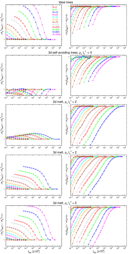
Refer to caption
Fig. S 1: Equilibration of 2d2𝑑2d and 3d3𝑑3d lattice trees of mass size N𝑁N via the “amoeba” algorithm (Sec. IIIA, main paper) for different ensembles, as a function of Monte Carlo time-steps (tMCsubscript𝑡𝑀𝐶t_{MC}). Left and right panels are for, respectively, the (ensemble-average) square gyration radius (Rg2(tMC)delimited-⟨⟩superscriptsubscript𝑅𝑔2subscript𝑡𝑀𝐶\langle R_{g}^{2}(t_{MC})\rangle) and number of branching nodes (n3(tMC)delimited-⟨⟩subscript𝑛3subscript𝑡𝑀𝐶\langle n_{3}(t_{MC})\rangle) normalized to the corresponding asymptotic values. For comparison, data for 3d3𝑑3d self-avoiding trees (i.e., zero density) from [Rosa & Everaers, J. Phys. A.: Math. Theor. 49, 345001 (2016)] are also reported. In all cases, the initial configuration for each tree corresponds to a linearly connected random walk.
Refer to caption
Fig. S 2: Branching statistics. Distribution functions for the number of branching points n3subscript𝑛3n_{3} (symbols) follow the Gaussian distribution (orange solid line). Corresponding variances σn32superscriptsubscript𝜎subscript𝑛32\sigma_{n_{3}}^{2} increase linearly with N𝑁N as: σn32/N=0.0410±0.0002superscriptsubscript𝜎subscript𝑛32𝑁plus-or-minus0.04100.0002\sigma_{n_{3}}^{2}/N=0.0410\pm 0.0002 (ideal trees); σn32/N=0.0447±0.0002superscriptsubscript𝜎subscript𝑛32𝑁plus-or-minus0.04470.0002\sigma_{n_{3}}^{2}/N=0.0447\pm 0.0002 (2d2𝑑2d melt of trees, ρKlK2=2subscript𝜌𝐾superscriptsubscript𝑙𝐾22\rho_{K}l_{K}^{2}=2); σn32/N=0.0428±0.0003superscriptsubscript𝜎subscript𝑛32𝑁plus-or-minus0.04280.0003\sigma_{n_{3}}^{2}/N=0.0428\pm 0.0003 (3d3𝑑3d melt of trees, ρKlK3=2subscript𝜌𝐾superscriptsubscript𝑙𝐾32\rho_{K}l_{K}^{3}=2); σn32/N=0.0424±0.0002superscriptsubscript𝜎subscript𝑛32𝑁plus-or-minus0.04240.0002\sigma_{n_{3}}^{2}/N=0.0424\pm 0.0002 (3d3𝑑3d melt of trees, ρKlK3=5subscript𝜌𝐾superscriptsubscript𝑙𝐾35\rho_{K}l_{K}^{3}=5).
Refer to caption
Fig. S 3: Path length statistics. (Left) Average contour distance of nodes from the central node, δLcenter(N)delimited-⟨⟩𝛿subscript𝐿center𝑁\langle\delta L_{\mathrm{center}}(N)\rangle. (Right) Average longest contour distance of nodes from the central node, δLcentermax(N)delimited-⟨⟩𝛿superscriptsubscript𝐿centermax𝑁\langle\delta L_{\mathrm{center}}^{\mathrm{max}}(N)\rangle. Straight lines correspond to the large-N𝑁N behaviour δLcenter(N)δLcentermax(N)Nρsimilar-todelimited-⟨⟩𝛿subscript𝐿center𝑁delimited-⟨⟩𝛿superscriptsubscript𝐿centermax𝑁similar-tosuperscript𝑁𝜌\langle\delta L_{\mathrm{center}}(N)\rangle\sim\langle\delta L_{\mathrm{center}}^{\mathrm{max}}(N)\rangle\sim N^{\rho} with critical exponents ρ𝜌\rho given by the best estimates summarised in Table I (main paper) and Table S4.

II Supplementary Tables

2d2𝑑2d ideal trees 3d3𝑑3d ideal trees
N𝑁N M𝑀M R𝑅R τMCsubscript𝜏𝑀𝐶\tau_{MC} τMC/τcorrsubscript𝜏𝑀𝐶subscript𝜏𝑐𝑜𝑟𝑟\tau_{MC}/\tau_{corr} R𝑅R τMCsubscript𝜏𝑀𝐶\tau_{MC} τMC/τcorrsubscript𝜏𝑀𝐶subscript𝜏𝑐𝑜𝑟𝑟\tau_{MC}/\tau_{corr}
3 1 128001280012800 51035superscript1035\cdot 10^{3} 833absent833\approx 833 160001600016000 11041superscript1041\cdot 10^{4} 1500absent1500\approx 1500
5 1 112001120011200 51035superscript1035\cdot 10^{3} 208absent208\approx 208 640064006400 11041superscript1041\cdot 10^{4} 400absent400\approx 400
10 1 120001200012000 51035superscript1035\cdot 10^{3} 52absent52\approx 52 320032003200 11041superscript1041\cdot 10^{4} 100absent100\approx 100
20 1 120001200012000 51035superscript1035\cdot 10^{3} 13absent13\approx 13 250002500025000 11041superscript1041\cdot 10^{4} 25absent25\approx 25
30 1 128001280012800 11041superscript1041\cdot 10^{4} 10absent10\approx 10 256002560025600 21042superscript1042\cdot 10^{4} 20absent20\approx 20
45 1 320003200032000 2.51042.5superscript1042.5\cdot 10^{4} 10absent10\approx 10 256002560025600 51045superscript1045\cdot 10^{4} 20absent20\approx 20
75 1 384003840038400 11051superscript1051\cdot 10^{5} 10absent10\approx 10 256002560025600 21052superscript1052\cdot 10^{5} 20absent20\approx 20
150 1 300003000030000 51055superscript1055\cdot 10^{5} 7absent7\approx 7 256002560025600 11061superscript1061\cdot 10^{6} 13absent13\approx 13
230 1 320003200032000 11061superscript1061\cdot 10^{6} 7absent7\approx 7 256002560025600 21062superscript1062\cdot 10^{6} 13absent13\approx 13
450 1 320003200032000 51065superscript1065\cdot 10^{6} 7absent7\approx 7 256002560025600 11071superscript1071\cdot 10^{7} 13absent13\approx 13
900 1 160001600016000 21072superscript1072\cdot 10^{7} 7absent7\approx 7 128001280012800 41074superscript1074\cdot 10^{7} 13absent13\approx 13
1800 1 800080008000 11081superscript1081\cdot 10^{8} 7absent7\approx 7 640064006400 21082superscript1082\cdot 10^{8} 13absent13\approx 13
2d2𝑑2d melt of trees, ρKlK2=2subscript𝜌𝐾superscriptsubscript𝑙𝐾22\rho_{K}l_{K}^{2}=2 3d3𝑑3d melt of trees, ρKlK3=2subscript𝜌𝐾superscriptsubscript𝑙𝐾32\rho_{K}l_{K}^{3}=2 3d3𝑑3d melt of trees, ρKlK3=5subscript𝜌𝐾superscriptsubscript𝑙𝐾35\rho_{K}l_{K}^{3}=5
N𝑁N M𝑀M R𝑅R τMCsubscript𝜏𝑀𝐶\tau_{MC} τMC/τcorrsubscript𝜏𝑀𝐶subscript𝜏𝑐𝑜𝑟𝑟\tau_{MC}/\tau_{corr} M𝑀M R𝑅R τMCsubscript𝜏𝑀𝐶\tau_{MC} τMC/τcorrsubscript𝜏𝑀𝐶subscript𝜏𝑐𝑜𝑟𝑟\tau_{MC}/\tau_{corr} M𝑀M R𝑅R τMCsubscript𝜏𝑀𝐶\tau_{MC} τMC/τcorrsubscript𝜏𝑀𝐶subscript𝜏𝑐𝑜𝑟𝑟\tau_{MC}/\tau_{corr}
3 128128128 100100100 21042superscript1042\cdot 10^{4} 600absent600\approx 600 256256256 100100100 21042superscript1042\cdot 10^{4} 800absent800\approx 800 160160160 100100100 11041superscript1041\cdot 10^{4} 400absent400\approx 400
5 112112112 100100100 21042superscript1042\cdot 10^{4} 150absent150\approx 150 256256256 100100100 21042superscript1042\cdot 10^{4} 200absent200\approx 200 646464 100100100 11041superscript1041\cdot 10^{4} 150absent150\approx 150
10 120120120 100100100 21042superscript1042\cdot 10^{4} 10absent10\approx 10 200200200 100100100 21042superscript1042\cdot 10^{4} 20absent20\approx 20 323232 100100100 11041superscript1041\cdot 10^{4} 26absent26\approx 26
20 120120120 100100100 21042superscript1042\cdot 10^{4} 3absent3\approx 3 288288288 100100100 21042superscript1042\cdot 10^{4} 3absent3\approx 3 250250250 100100100 11041superscript1041\cdot 10^{4} 3absent3\approx 3
30 128128128 100100100 11051superscript1051\cdot 10^{5} 4absent4\approx 4 336336336 100100100 11051superscript1051\cdot 10^{5} 6absent6\approx 6 256256256 100100100 21042superscript1042\cdot 10^{4} 3absent3\approx 3
45 320320320 100100100 2.51052.5superscript1052.5\cdot 10^{5} 3absent3\approx 3 256256256 100100100 2.51052.5superscript1052.5\cdot 10^{5} 6absent6\approx 6 256256256 100100100 51045superscript1045\cdot 10^{4} 3absent3\approx 3
75 384384384 100100100 1.81061.8superscript1061.8\cdot 10^{6} 6absent6\approx 6 256256256 100100100 1.81061.8superscript1061.8\cdot 10^{6} 10absent10\approx 10 256256256 100100100 21052superscript1052\cdot 10^{5} 3absent3\approx 3
150 300300300 100100100 8.41068.4superscript1068.4\cdot 10^{6} 4absent4\approx 4 288288288 100100100 8.41068.4superscript1068.4\cdot 10^{6} 8absent8\approx 8 256256256 100100100 11061superscript1061\cdot 10^{6} 2absent2\approx 2
230 288288288 100100100 2.21072.2superscript1072.2\cdot 10^{7} 3absent3\approx 3 264264264 100100100 2.21072.2superscript1072.2\cdot 10^{7} 8absent8\approx 8 256256256 100100100 21062superscript1062\cdot 10^{6} 2absent2\approx 2
450 320320320 100100100 1.41081.4superscript1081.4\cdot 10^{8} 3absent3\approx 3 256256256 100100100 11081superscript1081\cdot 10^{8} 6absent6\approx 6 256256256 100100100 11071superscript1071\cdot 10^{7} 2absent2\approx 2
900 888888 100100100 8.71088.7superscript1088.7\cdot 10^{8} 3absent3\approx 3 727272 100100100 41084superscript1084\cdot 10^{8} 6absent6\approx 6 128128128 100100100 41074superscript1074\cdot 10^{7} 2absent2\approx 2
1800 646464 100100100 21082superscript1082\cdot 10^{8} 2absent2\approx 2
Table S 1: Summary of MC results for trees from different ensembles. N𝑁N: number of Kuhn segments per tree. R𝑅R: total number of independent runs. M𝑀M: total number of trees per run. τMCsubscript𝜏𝑀𝐶\tau_{MC}: MC steps per single runsingle treeMC steps per single runsingle tree\frac{\mbox{MC steps per single run}}{\mbox{single tree}}. τMC/τcorrsubscript𝜏𝑀𝐶subscript𝜏𝑐𝑜𝑟𝑟\tau_{MC}/\tau_{corr}: total number of uncorrelated MC configurations per MC run. τcorrsubscript𝜏𝑐𝑜𝑟𝑟\tau_{corr} is the correlation time estimated via g3(τcorr)Rg2subscript𝑔3subscript𝜏𝑐𝑜𝑟𝑟delimited-⟨⟩superscriptsubscript𝑅𝑔2g_{3}(\tau_{corr})\approx\langle R_{g}^{2}\rangle (see also Fig. 2, main paper) where: g3(τ)subscript𝑔3𝜏g_{3}(\tau) is the mean-square displacement of the tree center of mass as a function of MC steps and Rg2delimited-⟨⟩superscriptsubscript𝑅𝑔2\langle R_{g}^{2}\rangle is the tree mean-square gyration radius.
N𝑁N n3delimited-⟨⟩subscript𝑛3\langle n_{3}\rangle δLcenterdelimited-⟨⟩𝛿subscript𝐿center\langle\delta L_{\mathrm{center}}\rangle δLcentermaxdelimited-⟨⟩𝛿superscriptsubscript𝐿centermax\langle\delta L_{\mathrm{center}}^{\mathrm{max}}\rangle Ldelimited-⟨⟩𝐿\langle L\rangle Nbrdelimited-⟨⟩subscript𝑁𝑏𝑟\langle N_{br}\rangle
2d2𝑑2d ideal trees
3 0.718±0.004plus-or-minus0.7180.0040.718\pm 0.004 0.821±0.001plus-or-minus0.8210.0010.821\pm 0.001 1.282±0.004plus-or-minus1.2820.0041.282\pm 0.004 1.160±0.001plus-or-minus1.1600.0011.160\pm 0.001 0.094±0.001plus-or-minus0.0940.0010.094\pm 0.001
5 1.429±0.006plus-or-minus1.4290.0061.429\pm 0.006 1.220±0.001plus-or-minus1.2200.0011.220\pm 0.001 2.033±0.002plus-or-minus2.0330.0022.033\pm 0.002 1.692±0.001plus-or-minus1.6920.0011.692\pm 0.001 0.464±0.001plus-or-minus0.4640.0010.464\pm 0.001
10 3.334±0.006plus-or-minus3.3340.0063.334\pm 0.006 1.932±0.002plus-or-minus1.9320.0021.932\pm 0.002 3.335±0.004plus-or-minus3.3350.0043.335\pm 0.004 2.763±0.001plus-or-minus2.7630.0012.763\pm 0.001 1.093±0.002plus-or-minus1.0930.0021.093\pm 0.002
20 7.292±0.009plus-or-minus7.2920.0097.292\pm 0.009 3.035±0.003plus-or-minus3.0350.0033.035\pm 0.003 5.394±0.007plus-or-minus5.3940.0075.394\pm 0.007 4.399±0.003plus-or-minus4.3990.0034.399\pm 0.003 2.129±0.003plus-or-minus2.1290.0032.129\pm 0.003
30 11.240±0.010plus-or-minus11.2400.01011.240\pm 0.010 3.922±0.004plus-or-minus3.9220.0043.922\pm 0.004 7.057±0.009plus-or-minus7.0570.0097.057\pm 0.009 5.716±0.003plus-or-minus5.7160.0035.716\pm 0.003 2.969±0.004plus-or-minus2.9690.0042.969\pm 0.004
45 17.206±0.008plus-or-minus17.2060.00817.206\pm 0.008 5.022±0.004plus-or-minus5.0220.0045.022\pm 0.004 9.129±0.007plus-or-minus9.1290.0079.129\pm 0.007 7.355±0.004plus-or-minus7.3550.0047.355\pm 0.004 4.016±0.003plus-or-minus4.0160.0034.016\pm 0.003
75 29.102±0.009plus-or-minus29.1020.00929.102\pm 0.009 6.811±0.005plus-or-minus6.8110.0056.811\pm 0.005 12.521±0.009plus-or-minus12.5210.00912.521\pm 0.009 10.018±0.005plus-or-minus10.0180.00510.018\pm 0.005 5.714±0.005plus-or-minus5.7140.0055.714\pm 0.005
150 58.862±0.013plus-or-minus58.8620.01358.862\pm 0.013 10.120±0.008plus-or-minus10.1200.00810.120\pm 0.008 18.881±0.016plus-or-minus18.8810.01618.881\pm 0.016 14.967±0.009plus-or-minus14.9670.00914.967\pm 0.009 8.865±0.009plus-or-minus8.8650.0098.865\pm 0.009
230 90.591±0.018plus-or-minus90.5910.01890.591\pm 0.018 12.818±0.011plus-or-minus12.8180.01112.818\pm 0.011 24.112±0.020plus-or-minus24.1120.02024.112\pm 0.020 19.011±0.012plus-or-minus19.0110.01219.011\pm 0.012 11.438±0.011plus-or-minus11.4380.01111.438\pm 0.011
450 177.938±0.024plus-or-minus177.9380.024177.938\pm 0.024 18.471±0.016plus-or-minus18.4710.01618.471\pm 0.016 35.137±0.030plus-or-minus35.1370.03035.137\pm 0.030 27.485±0.018plus-or-minus27.4850.01827.485\pm 0.018 16.836±0.017plus-or-minus16.8360.01716.836\pm 0.017
900 356.508±0.050plus-or-minus356.5080.050356.508\pm 0.050 26.702±0.035plus-or-minus26.7020.03526.702\pm 0.035 51.313±0.063plus-or-minus51.3130.06351.313\pm 0.063 39.818±0.034plus-or-minus39.8180.03439.818\pm 0.034 24.691±0.035plus-or-minus24.6910.03524.691\pm 0.035
1800 713.623±0.092plus-or-minus713.6230.092713.623\pm 0.092 38.250±0.071plus-or-minus38.2500.07138.250\pm 0.071 74.029±0.128plus-or-minus74.0290.12874.029\pm 0.128 57.161±0.084plus-or-minus57.1610.08457.161\pm 0.084 35.734±0.065plus-or-minus35.7340.06535.734\pm 0.065
3d3𝑑3d ideal trees
3 0.709±0.003plus-or-minus0.7090.0030.709\pm 0.003 0.823±0.001plus-or-minus0.8230.0010.823\pm 0.001 1.291±0.003plus-or-minus1.2910.0031.291\pm 0.003 1.161±0.001plus-or-minus1.1610.0011.161\pm 0.001 0.097±0.001plus-or-minus0.0970.0010.097\pm 0.001
5 1.450±0.015plus-or-minus1.4500.0151.450\pm 0.015 1.220±0.001plus-or-minus1.2200.0011.220\pm 0.001 2.030±0.002plus-or-minus2.0300.0022.030\pm 0.002 1.692±0.001plus-or-minus1.6920.0011.692\pm 0.001 0.464±0.001plus-or-minus0.4640.0010.464\pm 0.001
10 3.320±0.012plus-or-minus3.3200.0123.320\pm 0.012 1.938±0.003plus-or-minus1.9380.0031.938\pm 0.003 3.357±0.009plus-or-minus3.3570.0093.357\pm 0.009 2.769±0.003plus-or-minus2.7690.0032.769\pm 0.003 1.098±0.003plus-or-minus1.0980.0031.098\pm 0.003
20 7.305±0.006plus-or-minus7.3050.0067.305\pm 0.006 3.036±0.002plus-or-minus3.0360.0023.036\pm 0.002 5.393±0.004plus-or-minus5.3930.0045.393\pm 0.004 4.399±0.002plus-or-minus4.3990.0024.399\pm 0.002 2.131±0.002plus-or-minus2.1310.0022.131\pm 0.002
30 11.256±0.007plus-or-minus11.2560.00711.256\pm 0.007 3.923±0.003plus-or-minus3.9230.0033.923\pm 0.003 7.054±0.005plus-or-minus7.0540.0057.054\pm 0.005 5.715±0.003plus-or-minus5.7150.0035.715\pm 0.003 2.971±0.003plus-or-minus2.9710.0032.971\pm 0.003
45 17.202±0.008plus-or-minus17.2020.00817.202\pm 0.008 5.025±0.004plus-or-minus5.0250.0045.025\pm 0.004 9.137±0.007plus-or-minus9.1370.0079.137\pm 0.007 7.358±0.004plus-or-minus7.3580.0047.358\pm 0.004 4.017±0.004plus-or-minus4.0170.0044.017\pm 0.004
75 29.120±0.012plus-or-minus29.1200.01229.120\pm 0.012 6.800±0.006plus-or-minus6.8000.0066.800\pm 0.006 12.512±0.011plus-or-minus12.5120.01112.512\pm 0.011 10.008±0.006plus-or-minus10.0080.00610.008\pm 0.006 5.706±0.006plus-or-minus5.7060.0065.706\pm 0.006
150 58.874±0.017plus-or-minus58.8740.01758.874\pm 0.017 10.124±0.010plus-or-minus10.1240.01010.124\pm 0.010 18.897±0.021plus-or-minus18.8970.02118.897\pm 0.021 14.974±0.010plus-or-minus14.9740.01014.974\pm 0.010 8.874±0.011plus-or-minus8.8740.0118.874\pm 0.011
230 90.614±0.019plus-or-minus90.6140.01990.614\pm 0.019 12.834±0.012plus-or-minus12.8340.01212.834\pm 0.012 24.137±0.023plus-or-minus24.1370.02324.137\pm 0.023 19.027±0.013plus-or-minus19.0270.01319.027\pm 0.013 11.453±0.011plus-or-minus11.4530.01111.453\pm 0.011
450 177.882±0.026plus-or-minus177.8820.026177.882\pm 0.026 18.510±0.018plus-or-minus18.5100.01818.510\pm 0.018 35.180±0.037plus-or-minus35.1800.03735.180\pm 0.037 27.526±0.020plus-or-minus27.5260.02027.526\pm 0.020 16.879±0.019plus-or-minus16.8790.01916.879\pm 0.019
900 356.425±0.051plus-or-minus356.4250.051356.425\pm 0.051 26.740±0.038plus-or-minus26.7400.03826.740\pm 0.038 51.330±0.069plus-or-minus51.3300.06951.330\pm 0.069 39.850±0.043plus-or-minus39.8500.04339.850\pm 0.043 24.724±0.039plus-or-minus24.7240.03924.724\pm 0.039
1800 713.491±0.101plus-or-minus713.4910.101713.491\pm 0.101 38.243±0.079plus-or-minus38.2430.07938.243\pm 0.079 74.043±0.129plus-or-minus74.0430.12974.043\pm 0.129 57.174±0.090plus-or-minus57.1740.09057.174\pm 0.090 35.723±0.073plus-or-minus35.7230.07335.723\pm 0.073
Table S 2: Connectivity and branching statistics of 2d2𝑑2d and 3d3𝑑3d ideal lattice trees of mass N𝑁N: n3delimited-⟨⟩subscript𝑛3\langle n_{3}\rangle, average number of three-functional nodes. δLcenterdelimited-⟨⟩𝛿subscript𝐿center\langle\delta L_{\mathrm{center}}\rangle, average path distance from the central node. δLcentermaxdelimited-⟨⟩𝛿superscriptsubscript𝐿centermax\langle\delta L_{\mathrm{center}}^{\mathrm{max}}\rangle, average longest path distance from the central node. Ldelimited-⟨⟩𝐿\langle L\rangle, average path distance between nodes. Nbrdelimited-⟨⟩subscript𝑁𝑏𝑟\langle N_{br}\rangle, average branch weight. Notice that statistics of ideal trees are independent of space dimensionality.
N𝑁N n3delimited-⟨⟩subscript𝑛3\langle n_{3}\rangle δLcenterdelimited-⟨⟩𝛿subscript𝐿center\langle\delta L_{\mathrm{center}}\rangle δLcentermaxdelimited-⟨⟩𝛿superscriptsubscript𝐿centermax\langle\delta L_{\mathrm{center}}^{\mathrm{max}}\rangle Ldelimited-⟨⟩𝐿\langle L\rangle Nbrdelimited-⟨⟩subscript𝑁𝑏𝑟\langle N_{br}\rangle
2d2𝑑2d melt of trees, ρKlK2=2subscript𝜌𝐾superscriptsubscript𝑙𝐾22\rho_{K}l_{K}^{2}=2
3 0.682±0.004plus-or-minus0.6820.0040.682\pm 0.004 0.829±0.001plus-or-minus0.8290.0010.829\pm 0.001 1.318±0.004plus-or-minus1.3180.0041.318\pm 0.004 1.165±0.001plus-or-minus1.1650.0011.165\pm 0.001 0.106±0.001plus-or-minus0.1060.0010.106\pm 0.001
5 1.414±0.005plus-or-minus1.4140.0051.414\pm 0.005 1.220±0.001plus-or-minus1.2200.0011.220\pm 0.001 2.039±0.002plus-or-minus2.0390.0022.039\pm 0.002 1.694±0.001plus-or-minus1.6940.0011.694\pm 0.001 0.464±0.001plus-or-minus0.4640.0010.464\pm 0.001
10 3.348±0.007plus-or-minus3.3480.0073.348\pm 0.007 1.935±0.002plus-or-minus1.9350.0021.935\pm 0.002 3.333±0.004plus-or-minus3.3330.0043.333\pm 0.004 2.764±0.001plus-or-minus2.7640.0012.764\pm 0.001 1.096±0.002plus-or-minus1.0960.0021.096\pm 0.002
20 7.395±0.010plus-or-minus7.3950.0107.395\pm 0.010 3.051±0.003plus-or-minus3.0510.0033.051\pm 0.003 5.432±0.007plus-or-minus5.4320.0075.432\pm 0.007 4.408±0.003plus-or-minus4.4080.0034.408\pm 0.003 2.147±0.003plus-or-minus2.1470.0032.147\pm 0.003
30 11.439±0.012plus-or-minus11.4390.01211.439\pm 0.012 3.956±0.004plus-or-minus3.9560.0043.956\pm 0.004 7.122±0.008plus-or-minus7.1220.0087.122\pm 0.008 5.744±0.004plus-or-minus5.7440.0045.744\pm 0.004 3.008±0.004plus-or-minus3.0080.0043.008\pm 0.004
45 17.472±0.008plus-or-minus17.4720.00817.472\pm 0.008 5.113±0.003plus-or-minus5.1130.0035.113\pm 0.003 9.307±0.007plus-or-minus9.3070.0079.307\pm 0.007 7.449±0.004plus-or-minus7.4490.0047.449\pm 0.004 4.112±0.003plus-or-minus4.1120.0034.112\pm 0.003
75 29.554±0.009plus-or-minus29.5540.00929.554\pm 0.009 7.043±0.005plus-or-minus7.0430.0057.043\pm 0.005 12.973±0.009plus-or-minus12.9730.00912.973\pm 0.009 10.285±0.005plus-or-minus10.2850.00510.285\pm 0.005 5.959±0.005plus-or-minus5.9590.0055.959\pm 0.005
150 59.770±0.016plus-or-minus59.7700.01659.770\pm 0.016 10.789±0.009plus-or-minus10.7890.00910.789\pm 0.009 20.152±0.016plus-or-minus20.1520.01620.152\pm 0.016 15.788±0.010plus-or-minus15.7880.01015.788\pm 0.010 9.554±0.008plus-or-minus9.5540.0089.554\pm 0.008
230 91.950±0.020plus-or-minus91.9500.02091.950\pm 0.020 13.996±0.012plus-or-minus13.9960.01213.996\pm 0.012 26.319±0.022plus-or-minus26.3190.02226.319\pm 0.022 20.499±0.014plus-or-minus20.4990.01420.499\pm 0.014 12.646±0.012plus-or-minus12.6460.01212.646\pm 0.012
450 180.556±0.030plus-or-minus180.5560.030180.556\pm 0.030 21.130±0.017plus-or-minus21.1300.01721.130\pm 0.017 40.094±0.032plus-or-minus40.0940.03240.094\pm 0.032 30.937±0.018plus-or-minus30.9370.01830.937\pm 0.018 19.524±0.016plus-or-minus19.5240.01619.524\pm 0.016
900 361.877±0.064plus-or-minus361.8770.064361.877\pm 0.064 32.303±0.051plus-or-minus32.3030.05132.303\pm 0.051 61.678±0.095plus-or-minus61.6780.09561.678\pm 0.095 47.284±0.055plus-or-minus47.2840.05547.284\pm 0.055 30.321±0.051plus-or-minus30.3210.05130.321\pm 0.051
3d3𝑑3d melt of trees, ρKlK3=2subscript𝜌𝐾superscriptsubscript𝑙𝐾32\rho_{K}l_{K}^{3}=2
3 0.671±0.003plus-or-minus0.6710.0030.671\pm 0.003 0.832±0.001plus-or-minus0.8320.0010.832\pm 0.001 1.329±0.003plus-or-minus1.3290.0031.329\pm 0.003 1.166±0.001plus-or-minus1.1660.0011.166\pm 0.001 0.110±0.001plus-or-minus0.1100.0010.110\pm 0.001
5 1.411±0.004plus-or-minus1.4110.0041.411\pm 0.004 1.220±0.001plus-or-minus1.2200.0011.220\pm 0.001 2.035±0.001plus-or-minus2.0350.0012.035\pm 0.001 1.694±0.001plus-or-minus1.6940.0011.694\pm 0.001 0.464±0.001plus-or-minus0.4640.0010.464\pm 0.001
10 3.340±0.004plus-or-minus3.3400.0043.340\pm 0.004 1.934±0.001plus-or-minus1.9340.0011.934\pm 0.001 3.334±0.003plus-or-minus3.3340.0033.334\pm 0.003 2.765±0.001plus-or-minus2.7650.0012.765\pm 0.001 1.096±0.001plus-or-minus1.0960.0011.096\pm 0.001
20 7.368±0.006plus-or-minus7.3680.0067.368\pm 0.006 3.040±0.002plus-or-minus3.0400.0023.040\pm 0.002 5.404±0.004plus-or-minus5.4040.0045.404\pm 0.004 4.401±0.002plus-or-minus4.4010.0024.401\pm 0.002 2.137±0.002plus-or-minus2.1370.0022.137\pm 0.002
30 11.409±0.007plus-or-minus11.4090.00711.409\pm 0.007 3.930±0.002plus-or-minus3.9300.0023.930\pm 0.002 7.065±0.005plus-or-minus7.0650.0057.065\pm 0.005 5.719±0.002plus-or-minus5.7190.0025.719\pm 0.002 2.980±0.002plus-or-minus2.9800.0022.980\pm 0.002
45 17.425±0.009plus-or-minus17.4250.00917.425\pm 0.009 5.067±0.004plus-or-minus5.0670.0045.067\pm 0.004 9.208±0.008plus-or-minus9.2080.0089.208\pm 0.008 7.399±0.004plus-or-minus7.3990.0047.399\pm 0.004 4.062±0.004plus-or-minus4.0620.0044.062\pm 0.004
75 29.510±0.012plus-or-minus29.5100.01229.510\pm 0.012 6.884±0.006plus-or-minus6.8840.0066.884\pm 0.006 12.667±0.011plus-or-minus12.6670.01112.667\pm 0.011 10.099±0.006plus-or-minus10.0990.00610.099\pm 0.006 5.789±0.006plus-or-minus5.7890.0065.789\pm 0.006
150 59.650±0.019plus-or-minus59.6500.01959.650\pm 0.019 10.361±0.009plus-or-minus10.3610.00910.361\pm 0.009 19.334±0.017plus-or-minus19.3340.01719.334\pm 0.017 15.263±0.010plus-or-minus15.2630.01015.263\pm 0.010 9.110±0.009plus-or-minus9.1100.0099.110\pm 0.009
230 91.770±0.019plus-or-minus91.7700.01991.770\pm 0.019 13.245±0.012plus-or-minus13.2450.01213.245\pm 0.012 24.894±0.023plus-or-minus24.8940.02324.894\pm 0.023 19.554±0.015plus-or-minus19.5540.01519.554\pm 0.015 11.866±0.012plus-or-minus11.8660.01211.866\pm 0.012
450 180.254±0.031plus-or-minus180.2540.031180.254\pm 0.031 19.282±0.019plus-or-minus19.2820.01919.282\pm 0.019 36.630±0.034plus-or-minus36.6300.03436.630\pm 0.034 28.564±0.022plus-or-minus28.5640.02228.564\pm 0.022 17.642±0.019plus-or-minus17.6420.01917.642\pm 0.019
900 361.189±0.077plus-or-minus361.1890.077361.189\pm 0.077 28.314±0.053plus-or-minus28.3140.05328.314\pm 0.053 54.216±0.097plus-or-minus54.2160.09754.216\pm 0.097 41.996±0.058plus-or-minus41.9960.05841.996\pm 0.058 26.288±0.054plus-or-minus26.2880.05426.288\pm 0.054
3d3𝑑3d melt of trees, ρKlK3=5subscript𝜌𝐾superscriptsubscript𝑙𝐾35\rho_{K}l_{K}^{3}=5
3 0.672±0.004plus-or-minus0.6720.0040.672\pm 0.004 0.832±0.001plus-or-minus0.8320.0010.832\pm 0.001 1.329±0.004plus-or-minus1.3290.0041.329\pm 0.004 1.166±0.001plus-or-minus1.1660.0011.166\pm 0.001 0.110±0.001plus-or-minus0.1100.0010.110\pm 0.001
5 1.367±0.025plus-or-minus1.3670.0251.367\pm 0.025 1.227±0.001plus-or-minus1.2270.0011.227\pm 0.001 2.047±0.003plus-or-minus2.0470.0032.047\pm 0.003 1.701±0.001plus-or-minus1.7010.0011.701\pm 0.001 0.473±0.002plus-or-minus0.4730.0020.473\pm 0.002
10 3.285±0.012plus-or-minus3.2850.0123.285\pm 0.012 1.942±0.003plus-or-minus1.9420.0031.942\pm 0.003 3.349±0.009plus-or-minus3.3490.0093.349\pm 0.009 2.774±0.003plus-or-minus2.7740.0032.774\pm 0.003 1.103±0.003plus-or-minus1.1030.0031.103\pm 0.003
20 7.209±0.006plus-or-minus7.2090.0067.209\pm 0.006 3.053±0.002plus-or-minus3.0530.0023.053\pm 0.002 5.434±0.004plus-or-minus5.4340.0045.434\pm 0.004 4.418±0.002plus-or-minus4.4180.0024.418\pm 0.002 2.147±0.002plus-or-minus2.1470.0022.147\pm 0.002
30 11.167±0.006plus-or-minus11.1670.00611.167\pm 0.006 3.940±0.003plus-or-minus3.9400.0033.940\pm 0.003 7.098±0.006plus-or-minus7.0980.0067.098\pm 0.006 5.737±0.003plus-or-minus5.7370.0035.737\pm 0.003 2.988±0.003plus-or-minus2.9880.0032.988\pm 0.003
45 17.093±0.008plus-or-minus17.0930.00817.093\pm 0.008 5.051±0.004plus-or-minus5.0510.0045.051\pm 0.004 9.192±0.009plus-or-minus9.1920.0099.192\pm 0.009 7.392±0.004plus-or-minus7.3920.0047.392\pm 0.004 4.042±0.004plus-or-minus4.0420.0044.042\pm 0.004
75 28.949±0.011plus-or-minus28.9490.01128.949\pm 0.011 6.861±0.006plus-or-minus6.8610.0066.861\pm 0.006 12.629±0.010plus-or-minus12.6290.01012.629\pm 0.010 10.082±0.006plus-or-minus10.0820.00610.082\pm 0.006 5.765±0.005plus-or-minus5.7650.0055.765\pm 0.005
150 58.610±0.015plus-or-minus58.6100.01558.610\pm 0.015 10.242±0.009plus-or-minus10.2420.00910.242\pm 0.009 19.127±0.017plus-or-minus19.1270.01719.127\pm 0.017 15.125±0.010plus-or-minus15.1250.01015.125\pm 0.010 8.986±0.010plus-or-minus8.9860.0108.986\pm 0.010
230 90.164±0.020plus-or-minus90.1640.02090.164\pm 0.020 13.034±0.012plus-or-minus13.0340.01213.034\pm 0.012 24.514±0.020plus-or-minus24.5140.02024.514\pm 0.020 19.289±0.013plus-or-minus19.2890.01319.289\pm 0.013 11.655±0.010plus-or-minus11.6550.01011.655\pm 0.010
450 177.134±0.027plus-or-minus177.1340.027177.134\pm 0.027 18.955±0.019plus-or-minus18.9550.01918.955\pm 0.019 36.011±0.034plus-or-minus36.0110.03436.011\pm 0.034 28.104±0.021plus-or-minus28.1040.02128.104\pm 0.021 17.309±0.018plus-or-minus17.3090.01817.309\pm 0.018
900 354.864±0.062plus-or-minus354.8640.062354.864\pm 0.062 27.738±0.040plus-or-minus27.7380.04027.738\pm 0.040 53.183±0.064plus-or-minus53.1830.06453.183\pm 0.064 41.209±0.045plus-or-minus41.2090.04541.209\pm 0.045 25.716±0.034plus-or-minus25.7160.03425.716\pm 0.034
1800 710.024±0.110plus-or-minus710.0240.110710.024\pm 0.110 39.850±0.082plus-or-minus39.8500.08239.850\pm 0.082 78.622±0.154plus-or-minus78.6220.15478.622\pm 0.154 59.424±0.092plus-or-minus59.4240.09259.424\pm 0.092 37.310±0.077plus-or-minus37.3100.07737.310\pm 0.077
Table S 3: Connectivity and branching statistics of 2d2𝑑2d and 3d3𝑑3d melts of trees of mass N𝑁N with average density of Kuhn segments per unit cell ρKlKdsubscript𝜌𝐾superscriptsubscript𝑙𝐾𝑑\rho_{K}l_{K}^{d}. Symbols as in Table S2.
δLcenterNρsimilar-todelimited-⟨⟩𝛿subscript𝐿centersuperscript𝑁𝜌\langle\delta L_{\mathrm{center}}\rangle\sim N^{\rho} δLcentermaxNρsimilar-todelimited-⟨⟩𝛿superscriptsubscript𝐿centermaxsuperscript𝑁𝜌\langle\delta L_{\mathrm{center}}^{\mathrm{max}}\rangle\sim N^{\rho} LNρsimilar-todelimited-⟨⟩𝐿superscript𝑁𝜌\langle L\rangle\sim N^{\rho} NbrNϵsimilar-todelimited-⟨⟩subscript𝑁𝑏𝑟superscript𝑁italic-ϵ\langle N_{br}\rangle\sim N^{\epsilon}
Ideal trees
ΔΔ\Delta 0.239±0.045plus-or-minus0.2390.0450.239\pm 0.045 0.280±0.044plus-or-minus0.2800.0440.280\pm 0.044 0.271±0.028plus-or-minus0.2710.0280.271\pm 0.028 0.706±0.032plus-or-minus0.7060.0320.706\pm 0.032
χ~2superscript~𝜒2{\tilde{\chi}}^{2} 1.6721.6721.672 1.0731.0731.073 2.3552.3552.355 2.7062.7062.706
𝒬𝒬{\mathcal{Q}} 0.1230.1230.123 0.3760.3760.376 0.0280.0280.028 0.0130.0130.013
ρ=0.446±0.013𝜌plus-or-minus0.4460.013\rho=0.446\pm 0.013 ρ=0.467±0.010𝜌plus-or-minus0.4670.010\rho=0.467\pm 0.010 ρ=0.457±0.007𝜌plus-or-minus0.4570.007\rho=0.457\pm 0.007 ϵ=0.529±0.002italic-ϵplus-or-minus0.5290.002\epsilon=0.529\pm 0.002
ΔΔ\Delta 00 00 00 00
χ~2superscript~𝜒2{\tilde{\chi}}^{2} 7.4247.4247.424 11.39911.39911.399 10.47610.47610.476 12.17212.17212.172
𝒬𝒬{\mathcal{Q}} 0.0060.0060.006 0.0010.0010.001 0.0010.0010.001 0.0010.0010.001
ρ=0.525±0.002𝜌plus-or-minus0.5250.002\rho=0.525\pm 0.002 ρ=0.538±0.001𝜌plus-or-minus0.5380.001\rho=0.538\pm 0.001 ρ=0.529±0.001𝜌plus-or-minus0.5290.001\rho=0.529\pm 0.001 ϵ=0.543±0.002italic-ϵplus-or-minus0.5430.002\epsilon=0.543\pm 0.002
ρ=0.494±0.013±0.038𝜌plus-or-minus0.4940.0130.038\mathbf{\rho=0.494\pm 0.013\pm 0.038} ϵ=0.536±0.002±0.007italic-ϵplus-or-minus0.5360.0020.007\mathbf{\epsilon=0.536\pm 0.002\pm 0.007}
2d2𝑑2d melt of trees, ρKlK2=2subscript𝜌𝐾superscriptsubscript𝑙𝐾22\rho_{K}l_{K}^{2}=2
ΔΔ\Delta 0.767±0.045plus-or-minus0.7670.0450.767\pm 0.045 0.726±0.048plus-or-minus0.7260.0480.726\pm 0.048 0.696±0.028plus-or-minus0.6960.0280.696\pm 0.028 0.871±0.069plus-or-minus0.8710.0690.871\pm 0.069
χ~2superscript~𝜒2{\tilde{\chi}}^{2} 2.7702.7702.770 1.6121.6121.612 4.8614.8614.861 0.8070.8070.807
𝒬𝒬{\mathcal{Q}} 0.0170.0170.017 0.1530.1530.153 0.00020.00020.0002 0.5440.5440.544
ρ=0.606±0.002𝜌plus-or-minus0.6060.002\rho=0.606\pm 0.002 ρ=0.616±0.002𝜌plus-or-minus0.6160.002\rho=0.616\pm 0.002 0.603±0.002plus-or-minus0.6030.0020.603\pm 0.002 ϵ=0.623±0.002italic-ϵplus-or-minus0.6230.002\epsilon=0.623\pm 0.002
ΔΔ\Delta 00 00 00 00
χ~2superscript~𝜒2{\tilde{\chi}}^{2} 0.1530.1530.153 2.8152.8152.815 0.1900.1900.190 10.60710.60710.607
𝒬𝒬{\mathcal{Q}} 0.6960.6960.696 0.0930.0930.093 0.6630.6630.663 0.0010.0010.001
ρ=0.613±0.001𝜌plus-or-minus0.6130.001\rho=0.613\pm 0.001 ρ=0.625±0.001𝜌plus-or-minus0.6250.001\rho=0.625\pm 0.001 ρ=0.613±0.001𝜌plus-or-minus0.6130.001\rho=0.613\pm 0.001 ϵ=0.643±0.001italic-ϵplus-or-minus0.6430.001\epsilon=0.643\pm 0.001
ρ=0.613±0.002±0.007𝜌plus-or-minus0.6130.0020.007\mathbf{\rho=0.613\pm 0.002\pm 0.007} ϵ=0.633±0.002±0.010italic-ϵplus-or-minus0.6330.0020.010\mathbf{\epsilon=0.633\pm 0.002\pm 0.010}
3d3𝑑3d melt of trees, ρKlK3=2subscript𝜌𝐾superscriptsubscript𝑙𝐾32\rho_{K}l_{K}^{3}=2
ΔΔ\Delta 0.192±0.061plus-or-minus0.1920.0610.192\pm 0.061 0.289±0.046plus-or-minus0.2890.0460.289\pm 0.046 0.248±0.033plus-or-minus0.2480.0330.248\pm 0.033 0.693±0.048plus-or-minus0.6930.0480.693\pm 0.048
χ~2superscript~𝜒2{\tilde{\chi}}^{2} 3.0463.0463.046 1.7951.7951.795 3.3033.3033.303 3.9633.9633.963
𝒬𝒬{\mathcal{Q}} 0.0090.0090.009 0.1100.1100.110 0.0060.0060.006 0.0010.0010.001
ρ=0.450±0.023𝜌plus-or-minus0.4500.023\rho=0.450\pm 0.023 ρ=0.497±0.012𝜌plus-or-minus0.4970.012\rho=0.497\pm 0.012 0.477±0.010plus-or-minus0.4770.0100.477\pm 0.010 ϵ=0.548±0.003italic-ϵplus-or-minus0.5480.003\epsilon=0.548\pm 0.003
ΔΔ\Delta 00 00 00 00
χ~2superscript~𝜒2{\tilde{\chi}}^{2} 1.6461.6461.646 6.0116.0116.011 7.0737.0737.073 11.76211.76211.762
𝒬𝒬{\mathcal{Q}} 0.2000.2000.200 0.0140.0140.014 0.0080.0080.008 0.0010.0010.001
ρ=0.558±0.001𝜌plus-or-minus0.5580.001\rho=0.558\pm 0.001 ρ=0.572±0.001𝜌plus-or-minus0.5720.001\rho=0.572\pm 0.001 ρ=0.561±0.001𝜌plus-or-minus0.5610.001\rho=0.561\pm 0.001 ϵ=0.586±0.002italic-ϵplus-or-minus0.5860.002\epsilon=0.586\pm 0.002
ρ=0.519±0.023±0.047𝜌plus-or-minus0.5190.0230.047\mathbf{\rho=0.519\pm 0.023\pm 0.047} ϵ=0.567±0.003±0.019italic-ϵplus-or-minus0.5670.0030.019\mathbf{\epsilon=0.567\pm 0.003\pm 0.019}
3d3𝑑3d melt of trees, ρKlK3=5subscript𝜌𝐾superscriptsubscript𝑙𝐾35\rho_{K}l_{K}^{3}=5
ΔΔ\Delta 0.301±0.037plus-or-minus0.3010.0370.301\pm 0.037 0.499±0.036plus-or-minus0.4990.0360.499\pm 0.036 0.344±0.023plus-or-minus0.3440.0230.344\pm 0.023 0.737±0.031plus-or-minus0.7370.0310.737\pm 0.031
χ~2superscript~𝜒2{\tilde{\chi}}^{2} 2.7242.7242.724 1.5341.5341.534 3.3813.3813.381 0.8930.8930.893
𝒬𝒬{\mathcal{Q}} 0.0120.0120.012 0.1630.1630.163 0.0030.0030.003 0.4990.4990.499
ρ=0.493±0.008𝜌plus-or-minus0.4930.008\rho=0.493\pm 0.008 ρ=0.540±0.003𝜌plus-or-minus0.5400.003\rho=0.540\pm 0.003 0.500±0.004plus-or-minus0.5000.0040.500\pm 0.004 ϵ=0.548±0.002italic-ϵplus-or-minus0.5480.002\epsilon=0.548\pm 0.002
ΔΔ\Delta 00 00 00 00
χ~2superscript~𝜒2{\tilde{\chi}}^{2} 25.13725.13725.137 0.0950.0950.095 36.14936.14936.149 45.57345.57345.573
𝒬𝒬{\mathcal{Q}} 106superscript10610^{-6} 0.7580.7580.758 <106absentsuperscript106<10^{-6} <106absentsuperscript106<10^{-6}
ρ=0.539±0.002𝜌plus-or-minus0.5390.002\rho=0.539\pm 0.002 ρ=0.563±0.001𝜌plus-or-minus0.5630.001\rho=0.563\pm 0.001 ρ=0.543±0.001𝜌plus-or-minus0.5430.001\rho=0.543\pm 0.001 ϵ=0.559±0.002italic-ϵplus-or-minus0.5590.002\epsilon=0.559\pm 0.002
ρ=0.530±0.008±0.025𝜌plus-or-minus0.5300.0080.025\mathbf{\rho=0.530\pm 0.008\pm 0.025} ϵ=0.554±0.002±0.006italic-ϵplus-or-minus0.5540.0020.006\mathbf{\epsilon=0.554\pm 0.002\pm 0.006}
Table S 4: Critical exponents ρ𝜌\rho and ϵitalic-ϵ\epsilon, describing path length (δLcenterδLcentermaxLNρsimilar-todelimited-⟨⟩𝛿subscript𝐿centerdelimited-⟨⟩𝛿superscriptsubscript𝐿centermaxsimilar-todelimited-⟨⟩𝐿similar-tosuperscript𝑁𝜌\langle\delta L_{\mathrm{center}}\rangle\sim\langle\delta L_{\mathrm{center}}^{\mathrm{max}}\rangle\sim\langle L\rangle\sim N^{\rho}) and branching statistics (Nbr(N)Nϵsimilar-todelimited-⟨⟩subscript𝑁𝑏𝑟𝑁superscript𝑁italic-ϵ\langle N_{br}(N)\rangle\sim N^{\epsilon}), respectively. Single estimates were obtained from best fits of data with N230𝑁230N\geq 230 (2d2𝑑2d and 3d3𝑑3d melt of trees for ρKlKd=2subscript𝜌𝐾superscriptsubscript𝑙𝐾𝑑2\rho_{K}l_{K}^{d}=2) and N450𝑁450N\geq 450 (ideal trees, 3d3𝑑3d melt of trees for ρKlK3=5subscript𝜌𝐾superscriptsubscript𝑙𝐾35\rho_{K}l_{K}^{3}=5) to simple power-law behaviour (Δ=0Δ0\Delta=0) and data with N10𝑁10N\geq 10 to power-law behaviour with a correction-to-scaling term (Δ>0Δ0\Delta>0). Final estimates (in boldface) show the corresponding averages. Uncertainties are reported as “± statistical error±systematic errorplus-or-minusplus-or-minus statistical errorsystematic error\pm\mbox{ statistical error}\pm\mbox{systematic error}”. For more details on fitting procedures and error estimation, see Sec. IIIC main paper.
N𝑁N R2(=𝚗𝚒𝚗𝚝(L(N)))delimited-⟨⟩superscript𝑅2𝚗𝚒𝚗𝚝delimited-⟨⟩𝐿𝑁\langle R^{2}(\ell={\tt nint}(\langle L(N)\rangle))\rangle Lmaxdelimited-⟨⟩subscript𝐿max\langle L_{\mathrm{max}}\rangle R2(Lmax)delimited-⟨⟩superscript𝑅2subscript𝐿max\langle R^{2}(L_{\mathrm{max}})\rangle Rg2delimited-⟨⟩superscriptsubscript𝑅𝑔2\left\langle R_{g}^{2}\right\rangle
2d2𝑑2d ideal trees
3 1.000±0.000plus-or-minus1.0000.0001.000\pm 0.000 2.282±0.004plus-or-minus2.2820.0042.282\pm 0.004 2.277±0.016plus-or-minus2.2770.0162.277\pm 0.016 0.581±0.002plus-or-minus0.5810.0020.581\pm 0.002
5 2.003±0.006plus-or-minus2.0030.0062.003\pm 0.006 3.571±0.005plus-or-minus3.5710.0053.571\pm 0.005 3.518±0.029plus-or-minus3.5180.0293.518\pm 0.029 0.845±0.003plus-or-minus0.8450.0030.845\pm 0.003
10 3.005±0.009plus-or-minus3.0050.0093.005\pm 0.009 6.225±0.007plus-or-minus6.2250.0076.225\pm 0.007 6.300±0.054plus-or-minus6.3000.0546.300\pm 0.054 1.389±0.005plus-or-minus1.3890.0051.389\pm 0.005
20 3.999±0.011plus-or-minus3.9990.0113.999\pm 0.011 10.290±0.012plus-or-minus10.2900.01210.290\pm 0.012 10.100±0.088plus-or-minus10.1000.08810.100\pm 0.088 2.195±0.008plus-or-minus2.1950.0082.195\pm 0.008
30 5.986±0.019plus-or-minus5.9860.0195.986\pm 0.019 13.617±0.016plus-or-minus13.6170.01613.617\pm 0.016 13.493±0.115plus-or-minus13.4930.11513.493\pm 0.115 2.851±0.011plus-or-minus2.8510.0112.851\pm 0.011
45 7.017±0.013plus-or-minus7.0170.0137.017\pm 0.013 17.755±0.014plus-or-minus17.7550.01417.755\pm 0.014 17.666±0.096plus-or-minus17.6660.09617.666\pm 0.096 3.684±0.009plus-or-minus3.6840.0093.684\pm 0.009
75 10.018±0.018plus-or-minus10.0180.01810.018\pm 0.018 24.545±0.018plus-or-minus24.5450.01824.545\pm 0.018 24.695±0.126plus-or-minus24.6950.12624.695\pm 0.126 5.031±0.011plus-or-minus5.0310.0115.031\pm 0.011
150 15.008±0.031plus-or-minus15.0080.03115.008\pm 0.031 37.266±0.032plus-or-minus37.2660.03237.266\pm 0.032 37.262±0.215plus-or-minus37.2620.21537.262\pm 0.215 7.500±0.022plus-or-minus7.5000.0227.500\pm 0.022
230 18.972±0.038plus-or-minus18.9720.03818.972\pm 0.038 47.726±0.040plus-or-minus47.7260.04047.726\pm 0.040 47.515±0.267plus-or-minus47.5150.26747.515\pm 0.267 9.467±0.022plus-or-minus9.4670.0229.467\pm 0.022
450 26.956±0.054plus-or-minus26.9560.05426.956\pm 0.054 69.778±0.060plus-or-minus69.7780.06069.778\pm 0.060 70.048±0.398plus-or-minus70.0480.39870.048\pm 0.398 13.720±0.034plus-or-minus13.7200.03413.720\pm 0.034
900 39.990±0.113plus-or-minus39.9900.11339.990\pm 0.113 102.128±0.125plus-or-minus102.1280.125102.128\pm 0.125 102.987±0.831plus-or-minus102.9870.831102.987\pm 0.831 19.904±0.064plus-or-minus19.9040.06419.904\pm 0.064
1800 57.094±0.227plus-or-minus57.0940.22757.094\pm 0.227 147.554±0.257plus-or-minus147.5540.257147.554\pm 0.257 148.062±1.680plus-or-minus148.0621.680148.062\pm 1.680 28.630±0.145plus-or-minus28.6300.14528.630\pm 0.145
3d3𝑑3d ideal trees
3 1.000±0.000plus-or-minus1.0000.0001.000\pm 0.000 2.291±0.004plus-or-minus2.2910.0042.291\pm 0.004 2.276±0.012plus-or-minus2.2760.0122.276\pm 0.012 0.578±0.001plus-or-minus0.5780.0010.578\pm 0.001
5 1.994±0.006plus-or-minus1.9940.0061.994\pm 0.006 3.566±0.007plus-or-minus3.5660.0073.566\pm 0.007 3.617±0.033plus-or-minus3.6170.0333.617\pm 0.033 0.851±0.010plus-or-minus0.8510.0100.851\pm 0.010
10 2.978±0.015plus-or-minus2.9780.0152.978\pm 0.015 6.257±0.014plus-or-minus6.2570.0146.257\pm 0.014 6.207±0.085plus-or-minus6.2070.0856.207\pm 0.085 1.323±0.028plus-or-minus1.3230.0281.323\pm 0.028
20 3.998±0.006plus-or-minus3.9980.0063.998\pm 0.006 10.287±0.009plus-or-minus10.2870.00910.287\pm 0.009 10.305±0.052plus-or-minus10.3050.05210.305\pm 0.052 2.199±0.005plus-or-minus2.1990.0052.199\pm 0.005
30 5.998±0.011plus-or-minus5.9980.0115.998\pm 0.011 13.615±0.011plus-or-minus13.6150.01113.615\pm 0.011 13.604±0.069plus-or-minus13.6040.06913.604\pm 0.069 2.857±0.006plus-or-minus2.8570.0062.857\pm 0.006
45 7.018±0.012plus-or-minus7.0180.0127.018\pm 0.012 17.774±0.015plus-or-minus17.7740.01517.774\pm 0.015 17.668±0.090plus-or-minus17.6680.09017.668\pm 0.090 3.688±0.008plus-or-minus3.6880.0083.688\pm 0.008
75 10.012±0.018plus-or-minus10.0120.01810.012\pm 0.018 24.526±0.022plus-or-minus24.5260.02224.526\pm 0.022 24.587±0.126plus-or-minus24.5870.12624.587\pm 0.126 5.006±0.012plus-or-minus5.0060.0125.006\pm 0.012
150 14.974±0.027plus-or-minus14.9740.02714.974\pm 0.027 37.291±0.035plus-or-minus37.2910.03537.291\pm 0.035 37.094±0.192plus-or-minus37.0940.19237.094\pm 0.192 7.468±0.016plus-or-minus7.4680.0167.468\pm 0.016
230 19.034±0.035plus-or-minus19.0340.03519.034\pm 0.035 47.774±0.045plus-or-minus47.7740.04547.774\pm 0.045 47.664±0.250plus-or-minus47.6640.25047.664\pm 0.250 9.528±0.021plus-or-minus9.5280.0219.528\pm 0.021
450 27.931±0.052plus-or-minus27.9310.05227.931\pm 0.052 69.862±0.067plus-or-minus69.8620.06769.862\pm 0.067 69.747±0.362plus-or-minus69.7470.36269.747\pm 0.362 13.718±0.028plus-or-minus13.7180.02813.718\pm 0.028
900 39.923±0.104plus-or-minus39.9230.10439.923\pm 0.104 102.155±0.139plus-or-minus102.1550.139102.155\pm 0.139 103.217±0.764plus-or-minus103.2170.764103.217\pm 0.764 19.936±0.063plus-or-minus19.9360.06319.936\pm 0.063
1800 57.296±0.208plus-or-minus57.2960.20857.296\pm 0.208 147.584±0.283plus-or-minus147.5840.283147.584\pm 0.283 149.921±1.575plus-or-minus149.9211.575149.921\pm 1.575 28.802±0.122plus-or-minus28.8020.12228.802\pm 0.122
Table S 5: Conformational statistics of 2d2𝑑2d and 3d3𝑑3d ideal lattice trees of mass N𝑁N: R2(=𝚗𝚒𝚗𝚝(L(N)))delimited-⟨⟩superscript𝑅2𝚗𝚒𝚗𝚝delimited-⟨⟩𝐿𝑁\langle R^{2}(\ell={\tt nint}(\langle L(N)\rangle))\rangle, average-square end-to-end distance of paths of length =𝚗𝚒𝚗𝚝(L(N))𝚗𝚒𝚗𝚝delimited-⟨⟩𝐿𝑁absent\ell={\tt nint}(\langle L(N)\rangle)\equiv closest-integer-to L(N)delimited-⟨⟩𝐿𝑁\langle L(N)\rangle. Lmaxdelimited-⟨⟩subscript𝐿max\langle L_{\mathrm{max}}\rangle, average length of the longest paths. R2(Lmax)delimited-⟨⟩superscript𝑅2subscript𝐿max\langle R^{2}(L_{\mathrm{max}})\rangle, average-square end-to-end distance of the longest paths. Rg2delimited-⟨⟩superscriptsubscript𝑅𝑔2\left\langle R_{g}^{2}\right\rangle, average-square gyration radius. As in Table S2, statistics of ideal trees is independent of space dimensionality.
N𝑁N R2(=𝚗𝚒𝚗𝚝(L(N)))delimited-⟨⟩superscript𝑅2𝚗𝚒𝚗𝚝delimited-⟨⟩𝐿𝑁\langle R^{2}(\ell={\tt nint}(\langle L(N)\rangle))\rangle Lmaxdelimited-⟨⟩subscript𝐿max\langle L_{\mathrm{max}}\rangle R2(Lmax)delimited-⟨⟩superscript𝑅2subscript𝐿max\langle R^{2}(L_{\mathrm{max}})\rangle Rg2delimited-⟨⟩superscriptsubscript𝑅𝑔2\left\langle R_{g}^{2}\right\rangle
2d2𝑑2d melt of trees, ρKlK2=2subscript𝜌𝐾superscriptsubscript𝑙𝐾22\rho_{K}l_{K}^{2}=2
3 1.000±0.000plus-or-minus1.0000.0001.000\pm 0.000 2.318±0.004plus-or-minus2.3180.0042.318\pm 0.004 2.453±0.017plus-or-minus2.4530.0172.453\pm 0.017 0.603±0.002plus-or-minus0.6030.0020.603\pm 0.002
5 2.181±0.005plus-or-minus2.1810.0052.181\pm 0.005 3.587±0.005plus-or-minus3.5870.0053.587\pm 0.005 4.102±0.031plus-or-minus4.1020.0314.102\pm 0.031 0.933±0.003plus-or-minus0.9330.0030.933\pm 0.003
10 3.690±0.008plus-or-minus3.6900.0083.690\pm 0.008 6.238±0.007plus-or-minus6.2380.0076.238\pm 0.007 8.250±0.061plus-or-minus8.2500.0618.250\pm 0.061 1.730±0.005plus-or-minus1.7300.0051.730\pm 0.005
20 5.552±0.009plus-or-minus5.5520.0095.552\pm 0.009 10.353±0.012plus-or-minus10.3530.01210.353\pm 0.012 16.281±0.122plus-or-minus16.2810.12216.281\pm 0.122 3.237±0.009plus-or-minus3.2370.0093.237\pm 0.009
30 9.597±0.018plus-or-minus9.5970.0189.597\pm 0.018 13.742±0.016plus-or-minus13.7420.01613.742\pm 0.016 24.101±0.172plus-or-minus24.1010.17224.101\pm 0.172 4.677±0.015plus-or-minus4.6770.0154.677\pm 0.015
45 12.083±0.012plus-or-minus12.0830.01212.083\pm 0.012 18.115±0.014plus-or-minus18.1150.01418.115\pm 0.014 35.009±0.157plus-or-minus35.0090.15735.009\pm 0.157 6.733±0.012plus-or-minus6.7330.0126.733\pm 0.012
75 20.219±0.019plus-or-minus20.2190.01920.219\pm 0.019 25.449±0.018plus-or-minus25.4490.01825.449\pm 0.018 57.527±0.233plus-or-minus57.5270.23357.527\pm 0.233 10.794±0.014plus-or-minus10.7940.01410.794\pm 0.014
150 40.727±0.043plus-or-minus40.7270.04340.727\pm 0.043 39.801±0.033plus-or-minus39.8010.03339.801\pm 0.033 112.627±0.508plus-or-minus112.6270.508112.627\pm 0.508 20.585±0.031plus-or-minus20.5850.03120.585\pm 0.031
230 57.661±0.059plus-or-minus57.6610.05957.661\pm 0.059 52.140±0.045plus-or-minus52.1400.04552.140\pm 0.045 170.895±0.778plus-or-minus170.8950.778170.895\pm 0.778 30.759±0.052plus-or-minus30.7590.05230.759\pm 0.052
450 113.568±0.111plus-or-minus113.5680.111113.568\pm 0.111 79.688±0.064plus-or-minus79.6880.06479.688\pm 0.064 328.627±1.392plus-or-minus328.6271.392328.627\pm 1.392 58.535±0.074plus-or-minus58.5350.07458.535\pm 0.074
900 220.202±0.396plus-or-minus220.2020.396220.202\pm 0.396 122.854±0.189plus-or-minus122.8540.189122.854\pm 0.189 651.115±5.217plus-or-minus651.1155.217651.115\pm 5.217 115.109±0.293plus-or-minus115.1090.293115.109\pm 0.293
3d3𝑑3d melt of trees, ρKlK3=2subscript𝜌𝐾superscriptsubscript𝑙𝐾32\rho_{K}l_{K}^{3}=2
3 1.000±0.000plus-or-minus1.0000.0001.000\pm 0.000 2.329±0.003plus-or-minus2.3290.0032.329\pm 0.003 2.404±0.010plus-or-minus2.4040.0102.404\pm 0.010 0.596±0.001plus-or-minus0.5960.0010.596\pm 0.001
5 2.099±0.003plus-or-minus2.0990.0032.099\pm 0.003 3.589±0.004plus-or-minus3.5890.0043.589\pm 0.004 3.907±0.017plus-or-minus3.9070.0173.907\pm 0.017 0.897±0.002plus-or-minus0.8970.0020.897\pm 0.002
10 3.406±0.005plus-or-minus3.4060.0053.406\pm 0.005 6.233±0.006plus-or-minus6.2330.0066.233\pm 0.006 7.423±0.037plus-or-minus7.4230.0377.423\pm 0.037 1.583±0.003plus-or-minus1.5830.0031.583\pm 0.003
20 4.849±0.005plus-or-minus4.8490.0054.849\pm 0.005 10.313±0.008plus-or-minus10.3130.00810.313\pm 0.008 13.348±0.056plus-or-minus13.3480.05613.348\pm 0.056 2.736±0.005plus-or-minus2.7360.0052.736\pm 0.005
30 7.773±0.009plus-or-minus7.7730.0097.773\pm 0.009 13.625±0.010plus-or-minus13.6250.01013.625\pm 0.010 18.401±0.073plus-or-minus18.4010.07318.401\pm 0.073 3.722±0.006plus-or-minus3.7220.0063.722\pm 0.006
45 9.373±0.012plus-or-minus9.3730.0129.373\pm 0.012 17.918±0.016plus-or-minus17.9180.01617.918\pm 0.016 25.342±0.117plus-or-minus25.3420.11725.342\pm 0.117 5.037±0.009plus-or-minus5.0370.0095.037\pm 0.009
75 14.213±0.019plus-or-minus14.2130.01914.213\pm 0.019 24.831±0.022plus-or-minus24.8310.02224.831\pm 0.022 36.610±0.170plus-or-minus36.6100.17036.610\pm 0.170 7.233±0.012plus-or-minus7.2330.0127.233\pm 0.012
150 22.944±0.029plus-or-minus22.9440.02922.944\pm 0.029 38.172±0.033plus-or-minus38.1720.03338.172\pm 0.033 60.550±0.270plus-or-minus60.5500.27060.550\pm 0.270 11.751±0.024plus-or-minus11.7510.02411.751\pm 0.024
230 32.153±0.046plus-or-minus32.1530.04632.153\pm 0.046 49.289±0.045plus-or-minus49.2890.04549.289\pm 0.045 80.884±0.383plus-or-minus80.8840.38380.884\pm 0.383 15.732±0.035plus-or-minus15.7320.03515.732\pm 0.035
450 50.246±0.072plus-or-minus50.2460.07250.246\pm 0.072 72.765±0.069plus-or-minus72.7650.06972.765\pm 0.069 128.880±0.616plus-or-minus128.8800.616128.880\pm 0.616 24.744±0.047plus-or-minus24.7440.04724.744\pm 0.047
900 77.753±0.205plus-or-minus77.7530.20577.753\pm 0.205 107.929±0.193plus-or-minus107.9290.193107.929\pm 0.193 202.464±1.867plus-or-minus202.4641.867202.464\pm 1.867 38.813±0.166plus-or-minus38.8130.16638.813\pm 0.166
3d3𝑑3d melt of trees, ρKlK3=5subscript𝜌𝐾superscriptsubscript𝑙𝐾35\rho_{K}l_{K}^{3}=5
3 1.000±0.000plus-or-minus1.0000.0001.000\pm 0.000 2.329±0.004plus-or-minus2.3290.0042.329\pm 0.004 2.385±0.013plus-or-minus2.3850.0132.385\pm 0.013 0.591±0.001plus-or-minus0.5910.0010.591\pm 0.001
5 2.031±0.006plus-or-minus2.0310.0062.031\pm 0.006 3.628±0.007plus-or-minus3.6280.0073.628\pm 0.007 3.710±0.033plus-or-minus3.7100.0333.710\pm 0.033 0.868±0.012plus-or-minus0.8680.0120.868\pm 0.012
10 3.161±0.014plus-or-minus3.1610.0143.161\pm 0.014 6.260±0.014plus-or-minus6.2600.0146.260\pm 0.014 6.789±0.088plus-or-minus6.7890.0886.789\pm 0.088 1.454±0.017plus-or-minus1.4540.0171.454\pm 0.017
20 4.305±0.006plus-or-minus4.3050.0064.305\pm 0.006 10.372±0.009plus-or-minus10.3720.00910.372\pm 0.009 11.488±0.055plus-or-minus11.4880.05511.488\pm 0.055 2.406±0.005plus-or-minus2.4060.0052.406\pm 0.005
30 6.636±0.011plus-or-minus6.6360.0116.636\pm 0.011 13.697±0.012plus-or-minus13.6970.01213.697\pm 0.012 15.403±0.075plus-or-minus15.4030.07515.403\pm 0.075 3.181±0.006plus-or-minus3.1810.0063.181\pm 0.006
45 7.875±0.012plus-or-minus7.8750.0127.875\pm 0.012 17.885±0.016plus-or-minus17.8850.01617.885\pm 0.016 20.719±0.100plus-or-minus20.7190.10020.719\pm 0.100 4.191±0.008plus-or-minus4.1910.0084.191\pm 0.008
75 11.572±0.018plus-or-minus11.5720.01811.572\pm 0.018 24.757±0.022plus-or-minus24.7570.02224.757\pm 0.022 29.073±0.143plus-or-minus29.0730.14329.073\pm 0.143 5.849±0.012plus-or-minus5.8490.0125.849\pm 0.012
150 18.007±0.029plus-or-minus18.0070.02918.007\pm 0.029 37.753±0.035plus-or-minus37.7530.03537.753\pm 0.035 46.095±0.227plus-or-minus46.0950.22746.095\pm 0.227 9.110±0.017plus-or-minus9.1100.0179.110\pm 0.017
230 23.296±0.037plus-or-minus23.2960.03723.296\pm 0.037 48.534±0.045plus-or-minus48.5340.04548.534\pm 0.045 60.730±0.300plus-or-minus60.7300.30060.730\pm 0.300 11.871±0.024plus-or-minus11.8710.02411.871\pm 0.024
450 35.781±0.057plus-or-minus35.7810.05735.781\pm 0.057 71.519±0.068plus-or-minus71.5190.06871.519\pm 0.068 91.625±0.456plus-or-minus91.6250.45691.625\pm 0.456 17.953±0.035plus-or-minus17.9530.03517.953\pm 0.035
900 54.530±0.121plus-or-minus54.5300.12154.530\pm 0.121 105.872±0.147plus-or-minus105.8720.147105.872\pm 0.147 141.131±0.990plus-or-minus141.1310.990141.131\pm 0.990 27.344±0.077plus-or-minus27.3440.07727.344\pm 0.077
1800 83.166±0.257plus-or-minus83.1660.25783.166\pm 0.257 153.467±0.296plus-or-minus153.4670.296153.467\pm 0.296 219.536±2.196plus-or-minus219.5362.196219.536\pm 2.196 41.237±0.164plus-or-minus41.2370.16441.237\pm 0.164
Table S 6: Conformational statistics of 2d2𝑑2d and 3d3𝑑3d melts of trees of mass N𝑁N with average density of Kuhn segments per unit cell ρKlKdsubscript𝜌𝐾superscriptsubscript𝑙𝐾𝑑\rho_{K}l_{K}^{d}. Symbols as in Table S5.
R2(=𝚗𝚒𝚗𝚝(L(N)))2νpathsimilar-todelimited-⟨⟩superscript𝑅2𝚗𝚒𝚗𝚝delimited-⟨⟩𝐿𝑁superscript2subscript𝜈path\langle R^{2}(\ell={\tt nint}(\langle L(N)\rangle))\rangle\sim\ell^{2\nu_{\mathrm{path}}} R2(Lmax)Lmax2νpathsimilar-todelimited-⟨⟩superscript𝑅2subscript𝐿maxsuperscriptdelimited-⟨⟩subscript𝐿max2subscript𝜈path\langle R^{2}(L_{\mathrm{max}})\rangle\sim\langle L_{\mathrm{max}}\rangle^{2\nu_{\mathrm{path}}} Rg2N2νsimilar-todelimited-⟨⟩superscriptsubscript𝑅𝑔2superscript𝑁2𝜈\left\langle R_{g}^{2}\right\rangle\sim N^{2\nu}
Ideal trees
ΔΔ\Delta 0.277±0.105plus-or-minus0.2770.1050.277\pm 0.105
χ~2superscript~𝜒2{\tilde{\chi}}^{2} 1.7701.7701.770
𝒬𝒬{\mathcal{Q}} 0.1010.1010.101
ν=0.229±0.013𝜈plus-or-minus0.2290.013\nu=0.229\pm 0.013
ΔΔ\Delta 00 00 00
χ~2superscript~𝜒2{\tilde{\chi}}^{2} 0.9990.9990.999 0.1120.1120.112 0.5620.5620.562
𝒬𝒬{\mathcal{Q}} 0.3180.3180.318 0.7380.7380.738 0.4540.4540.454
νpath=0.504±0.003subscript𝜈pathplus-or-minus0.5040.003\nu_{\mathrm{path}}=0.504\pm 0.003 νpath=0.513±0.007subscript𝜈pathplus-or-minus0.5130.007\nu_{\mathrm{path}}=0.513\pm 0.007 ν=0.268±0.002𝜈plus-or-minus0.2680.002\nu=0.268\pm 0.002
νpath=0.509±𝟎𝟎𝟕±0.005subscript𝜈pathplus-or-minus0.5090070.005\mathbf{\nu_{\mathrm{path}}=0.509\pm 007\pm 0.005} ν=0.249±0.013±0.020𝜈plus-or-minus0.2490.0130.020\mathbf{\nu=0.249\pm 0.013\pm 0.020}
2d2𝑑2d melt of trees, ρKlK2=2subscript𝜌𝐾superscriptsubscript𝑙𝐾22\rho_{K}l_{K}^{2}=2
ΔΔ\Delta
χ~2superscript~𝜒2{\tilde{\chi}}^{2}
𝒬𝒬{\mathcal{Q}}
ΔΔ\Delta 00 00 00
χ~2superscript~𝜒2{\tilde{\chi}}^{2} 44.03844.03844.038 1.7091.7091.709 8.5158.5158.515
𝒬𝒬{\mathcal{Q}} <106absentsuperscript106<10^{-6} 0.1910.1910.191 0.0040.0040.004
νpath=0.781±0.001subscript𝜈pathplus-or-minus0.7810.001\nu_{\mathrm{path}}=0.781\pm 0.001 νpath=0.778±0.005subscript𝜈pathplus-or-minus0.7780.005\nu_{\mathrm{path}}=0.778\pm 0.005 ν=0.483±0.001𝜈plus-or-minus0.4830.001\nu=0.483\pm 0.001
νpath=0.780±0.005±0.002subscript𝜈pathplus-or-minus0.7800.0050.002\mathbf{\nu_{\mathrm{path}}=0.780\pm 0.005\pm 0.002} ν=0.483±(0.008)±(0.013)𝜈plus-or-minus0.4830.0080.013\mathbf{\nu=0.483\pm(0.008)\pm(0.013)}
3d3𝑑3d melt of trees, ρKlK3=2subscript𝜌𝐾superscriptsubscript𝑙𝐾32\rho_{K}l_{K}^{3}=2
ΔΔ\Delta 0.384±0.086plus-or-minus0.3840.0860.384\pm 0.086
χ~2superscript~𝜒2{\tilde{\chi}}^{2} 1.4691.4691.469
𝒬𝒬{\mathcal{Q}} 0.1960.1960.196
ν=0.309±0.008𝜈plus-or-minus0.3090.008\nu=0.309\pm 0.008
ΔΔ\Delta 00 00 00
χ~2superscript~𝜒2{\tilde{\chi}}^{2} 4.0874.0874.087 1.9511.9511.951 6.9736.9736.973
𝒬𝒬{\mathcal{Q}} 0.0430.0430.043 0.1630.1630.163 0.0010.0010.001
νpath=0.597±0.002subscript𝜈pathplus-or-minus0.5970.002\nu_{\mathrm{path}}=0.597\pm 0.002 νpath=0.589±0.006subscript𝜈pathplus-or-minus0.5890.006\nu_{\mathrm{path}}=0.589\pm 0.006 ν=0.336±0.001𝜈plus-or-minus0.3360.001\nu=0.336\pm 0.001
νpath=0.593±0.006±0.004subscript𝜈pathplus-or-minus0.5930.0060.004\mathbf{\nu_{\mathrm{path}}=0.593\pm 0.006\pm 0.004} ν=0.323±0.008±0.013𝜈plus-or-minus0.3230.0080.013\mathbf{\nu=0.323\pm 0.008\pm 0.013}
3d3𝑑3d melt of trees, ρKlK3=5subscript𝜌𝐾superscriptsubscript𝑙𝐾35\rho_{K}l_{K}^{3}=5
ΔΔ\Delta 0.391±0.082plus-or-minus0.3910.0820.391\pm 0.082
χ~2superscript~𝜒2{\tilde{\chi}}^{2} 0.5080.5080.508
𝒬𝒬{\mathcal{Q}} 0.8030.8030.803
ν=0.286±0.007𝜈plus-or-minus0.2860.007\nu=0.286\pm 0.007
ΔΔ\Delta 00 00 00
χ~2superscript~𝜒2{\tilde{\chi}}^{2} 13.08913.08913.089 3.5243.5243.524 1.9271.9271.927
𝒬𝒬{\mathcal{Q}} 0.00030.00030.0003 0.0610.0610.061 0.1650.1650.165
νpath=0.563±0.002subscript𝜈pathplus-or-minus0.5630.002\nu_{\mathrm{path}}=0.563\pm 0.002 νpath=0.567±0.007subscript𝜈pathplus-or-minus0.5670.007\nu_{\mathrm{path}}=0.567\pm 0.007 ν=0.301±0.002𝜈plus-or-minus0.3010.002\nu=0.301\pm 0.002
νpath=0.565±0.007±0.002subscript𝜈pathplus-or-minus0.5650.0070.002\mathbf{\nu_{\mathrm{path}}=0.565\pm 0.007\pm 0.002} ν=0.294±0.007±0.008𝜈plus-or-minus0.2940.0070.008\mathbf{\nu=0.294\pm 0.007\pm 0.008}
Table S 7: Critical exponents νpathsubscript𝜈path\nu_{\mathrm{path}} and ν𝜈\nu describing, respectively, the scaling behaviors of R2(=𝚗𝚒𝚗𝚝(L(N)))2νpathsimilar-todelimited-⟨⟩superscript𝑅2𝚗𝚒𝚗𝚝delimited-⟨⟩𝐿𝑁superscript2subscript𝜈path\langle R^{2}(\ell={\tt nint}(\langle L(N)\rangle))\rangle\sim\ell^{2\nu_{\mathrm{path}}} and R2(Lmax)Lmax2νpathsimilar-todelimited-⟨⟩superscript𝑅2subscript𝐿maxsuperscriptdelimited-⟨⟩subscript𝐿max2subscript𝜈path\langle R^{2}(L_{\mathrm{max}})\rangle\sim\langle L_{\mathrm{max}}\rangle^{2\nu_{\mathrm{path}}}, and Rg2(N)N2νsimilar-todelimited-⟨⟩superscriptsubscript𝑅𝑔2𝑁superscriptdelimited-⟨⟩𝑁2𝜈\langle R_{g}^{2}(N)\rangle\sim\langle N\rangle^{2\nu}. Single estimates for ν𝜈\nu are the results of fitting the data to three- (Δ>0Δ0\Delta>0 for data with N10𝑁10N\geq 10) and two-parameter (Δ=0Δ0\Delta=0 for data with: N450𝑁450N\geq 450 (ideal trees, 3d3𝑑3d melt of trees for ρKlK3=5subscript𝜌𝐾superscriptsubscript𝑙𝐾35\rho_{K}l_{K}^{3}=5) and N230𝑁230N\geq 230 (2d2𝑑2d and 3d3𝑑3d melt of trees for ρKlKd=2subscript𝜌𝐾superscriptsubscript𝑙𝐾𝑑2\rho_{K}l_{K}^{d}=2)) functions, as described in Sec. IIIC main paper. In the case of 2d2𝑑2d melts where the three-parameter fit fails, corresponding statistical and systematic errors (in brackets) have been set to the same trends observed for 3d3𝑑3d melt of trees for ρKlK3=2subscript𝜌𝐾superscriptsubscript𝑙𝐾32\rho_{K}l_{K}^{3}=2. For the critical exponent νpathsubscript𝜈path\nu_{\mathrm{path}}, we have attempted similar analysis with two- and three-parameter fit functions: logR2(=𝚗𝚒𝚗𝚝(L(N)))=a+2νpathloglsuperscript𝑅2𝚗𝚒𝚗𝚝delimited-⟨⟩𝐿𝑁𝑎2subscript𝜈path𝑙\log\langle R^{2}(\ell={\tt nint}(\langle L(N)\rangle))\rangle=a+2\nu_{\mathrm{path}}\log l and logR2(=𝚗𝚒𝚗𝚝(L(N)))=a+blΔ0+2νpathloglb(ΔΔ0)lΔ0loglsuperscript𝑅2𝚗𝚒𝚗𝚝delimited-⟨⟩𝐿𝑁𝑎𝑏superscript𝑙subscriptΔ02subscript𝜈path𝑙𝑏ΔsubscriptΔ0superscript𝑙subscriptΔ0𝑙\log\langle R^{2}(\ell={\tt nint}(\langle L(N)\rangle))\rangle=a+b\,l^{-\Delta_{0}}+2\nu_{\mathrm{path}}\log l-b(\Delta-\Delta_{0})\,l^{-\Delta_{0}}\log l, and analogous expressions for Lmaxdelimited-⟨⟩subscript𝐿max\langle L_{\mathrm{max}}\rangle. Since three-parameter fits fail to produce reliable results, only estimates from two-parameter fits have been combined into our final values for νpathsubscript𝜈path\nu_{\mathrm{path}}.