Measuring quasiprobability distribution functions of the cavity field considering field and atomic decays

Abstract

We study the possibility of reconstructing the quantum state of light in a cavity subject to dissipation. We pass atoms, also subject to decay, through the cavity and surprisingly show that both decays allow the measurement of $s$-parametrized quasiprobability distributions. In fact, if we consider only atomic decay, we show that the Wigner function may be reconstructed. Because these distributions contain whole information of the initial field state, it is possible to recover information after both atomic and field decays occur.

1 Introduction

The measurement of a quantum state is a central topic in quantum optics and related fields [1, 2]. Several techniques have been developed in order to achieve such goal, for instance tomographic reconstruction by unbalanced homodyning [3], cascaded homodyning [4], the direct sampling of the density matrix of a signal mode in multiport optical homodyne tomography [5] and reconstruction via photocounting [6], to cite some. Proposals to measure electromagnetic fields inside cavities [7, 8] have also been given. Such state reconstruction in cavities is usually achieved through a finite set of selective measurements of atomic states [7] that make it possible to construct different quasiprobability distribution functions.

However, in real experiments, dissipative processes that have destructive effects may occur. Schemes that treat dissipative cavities have been proposed [8, 9]. They involve physical processes that allow the storage of information about quantum coherences of the initial state in the diagonal elements of the density matrix of a transformed state.

The relation between losses and $s$-parametrized quasiprobability distributions has already been pointed out by Leonhardt and Paul [10] and problems with the reconstruction of the Wigner function have been analyzed in [11]. Methods to reconstruct quasiprobability distribution functions in cavity QED are usually based on the expression [12]

$$F(\alpha,s)=\frac{1}{\pi(1-s)}\sum_{k=0}^{\infty}\left(\frac{s+1}{s-1}\right)^{k}\langle\alpha,k|\hat{\rho}|\alpha,k\rangle,$$ (1)

with $s$ as the parameter of quasiprobability function that indicates the relevant distribution ($s=-1$ Husimi [13], $s=0$ Wigner [14] and $s=1$ Glauber-Sudarshan [15, 16] distribution functions), $\rho$ the density matrix and the states $|\alpha,k\rangle$ are the so-called displaced number states [17].

Leibfried et al. [18] and Bertet et al. [19] used the above expression to measure the Wigner function ($s=0$ case) of the quantized motion of an ion and the quantized cavity field, respectively. It is possible to reconstruct a quasiprobability distribution function from the above equation since there is a direct recipe. Let us write equation (1) as

$$F(\alpha,s)=\frac{1}{\pi(1-s)}\sum_{k=0}^{\infty}\left(\frac{s+1}{s-1}\right)^{k}\langle k|\hat{D}^{\dagger}(\alpha)\hat{\rho}\hat{D}(\alpha)|k\rangle,$$ (2)

where $D(\alpha)$ is the Glauber displacement operator [15]. Note that, in order to obtain a quasiprobability distribution function we need to displace the system by an amplitude $\alpha$ and then measure the diagonal elements of the (displaced) density matrix.

We now aim to study the problem of reconstruction of the cavity field as studied in [20], however, not only cavity decay but also atomic decay is allowed [21]. We then want to show that it is still possible to recover whole information about the initial state through the reconstruction of $s$-parametrized quasiprobability distributions.

2 Dispersive interaction between a two-level atom and a quantized field

We consider the master equation for the dispersive interaction between a two-level atom and a quantized field

$$\frac{d\hat{\rho}}{dt}=-i\chi[\hat{n}\hat{\sigma}_{z},\hat{\rho}]+\hat{\mathcal{L}}_{F}\hat{\rho}+\hat{\mathcal{L}}_{A}\hat{\rho},$$ (3)

with $\chi$ as the dispersive interaction constant, $\hat{n}=\hat{a}^{\dagger}\hat{a}$ where $\hat{a}^{\dagger}$ and $\hat{a}$ are the creation and annihilation operators, respectively. $\hat{\sigma}_{z}$ is the Pauli-spin matrix related to the atomic inversion, and $\hat{\rho}$ is the density matrix of the atom-field system.

In the above equation the cavity and atomic decay terms are given by

$$\hat{\mathcal{L}}_{j}\hat{\rho}=(\hat{J}_{j}+\hat{L}_{j})\hat{\rho},\qquad j=A,F$$ (4)

in which the subscripts ”A” and ”F” refer to the terms atom and field, respectively. The corresponding superoperators are defined as

$$\hat{J}_{A}\hat{\rho}=2\Gamma\hat{\sigma}_{-}\hat{\rho}\hat{\sigma}_{+},\qquad\hat{J}_{F}\hat{\rho}=2\gamma\hat{a}\hat{\rho}\hat{a}^{\dagger},$$ (5)

and

$$\hat{L}_{A}\hat{\rho}=-\Gamma(\hat{\sigma}_{+}\hat{\sigma}_{-}\hat{\rho}+\hat{\rho}\hat{\sigma}_{+}\hat{\sigma}_{-}),\qquad\hat{L}_{F}\hat{\rho}=-\gamma(\hat{a}^{\dagger}\hat{a}\hat{\rho}+\hat{\rho}\hat{a}^{\dagger}\hat{a}).$$ (6)

We solve (3) by doing

$$\hat{\rho}(t)=e^{(\hat{R}+\hat{L}_{A}+\hat{L}_{F})t}e^{\int_{0}^{t}e^{-(\hat{R}+\hat{L}_{A}+\hat{L}_{F})t^{\prime}}(\hat{J}_{A}+\hat{J}_{F})e^{(\hat{R}+\hat{L}_{A}+\hat{L}_{F})t^{\prime}}dt^{\prime}}\hat{\rho}(0),$$ (7)

where we have defined

$$\hat{R}\rho=-i\chi\hat{\sigma}_{z}\hat{n}\hat{\rho}+i\chi\hat{\rho}\hat{\sigma}_{z}\hat{n}.$$ (8)

We note that

$$e^{-(\hat{R}+\hat{L}_{A}+\hat{L}_{F})t^{\prime}}(\hat{J}_{A}+\hat{J}_{F})e^{(\hat{R}+\hat{L}_{A}+\hat{L}_{F})t^{\prime}}\hat{\rho}$$ (9)

$$= \left(\hat{J}_{A}e^{-(\hat{R}_{F}+2\Gamma)t}+\hat{J}_{F}e^{-(\hat{R}_{A}+2\gamma)t}\right)\hat{\rho},$$ (10)

where the commutation relations

$$[\hat{L}_{A},\hat{J}_{A}]\hat{\rho}(t) = 2\Gamma\hat{J}_{A}\hat{\rho}(t),\qquad[\hat{L}_{F},\hat{J}_{F}]\hat{\rho}(t)=2\gamma\hat{J}_{F}\hat{\rho}(t),$$ (11)

and

$$[\hat{R},\hat{J}_{A}]\hat{\rho}(t)=\hat{J}_{A}(\hat{R}_{F}\hat{\rho}(t)),\qquad[\hat{R},\hat{J}_{F}]\hat{\rho}(t)=\hat{J}_{F}(\hat{R}_{A}\hat{\rho}(t)),$$ (12)

have been used. In the above equations, we have defined the superoperators $\hat{R}_{F}$ and $\hat{R}_{A}$ as

$$\hat{R}_{F}\hat{\rho}=2i\chi\hat{n}\hat{\rho}-2i\chi\hat{\rho}\hat{n},\qquad\hat{R}_{A}\hat{\rho}=i\chi\hat{\sigma}_{z}\hat{\rho}-i\chi\hat{\rho}\hat{\sigma}_{z},$$ (13)

which commute with all the other superoperators involved, such that the solution of the evolved density matrix is written as

$$\hat{\rho}(t)=e^{(\hat{R}+\hat{L}_{A}+\hat{L}_{F})t}e^{\hat{J}_{A}\frac{1-e^{-(\hat{R}_{F}+2\Gamma)t}}{\hat{R}_{F}+2\Gamma}}e^{\hat{J}_{F}\frac{1-e^{-(\hat{R}_{A}+2\gamma)t}}{\hat{R}_{A}+2\gamma}}\hat{\rho}(0).$$ (14)

One should note that, since $\hat{J}_{A}^{2}\hat{\rho}(t)=0$, the following simplification may be obtained

$$e^{\hat{J}_{A}\frac{1-e^{-(\hat{R}_{F}+2\Gamma)t}}{\hat{R}_{F}+2\Gamma}}\hat{\rho}(t)=\left(1+\hat{J}_{A}\frac{1-e^{-(\hat{R}_{F}+2\Gamma)t}}{\hat{R}_{F}+2\Gamma}\right)\hat{\rho}(t),$$ (15)

and therefore,

$$\hat{\rho}(t)=\hat{\rho}_{1}(t)+\hat{\rho}_{2}(t),$$ (16)

where

$$\hat{\rho}_{1}(t) = e^{t(\hat{R}+\hat{L}_{A}+\hat{L}_{F})}\ \ e^{\hat{J}_{F}\frac{1-e^{-(\hat{R}_{A}+2\gamma)t}}{\hat{R}_{A}+2\gamma}}\hat{\rho}(0),$$

$$\hat{\rho}_{2}(t) = e^{t(\hat{R}+\hat{L}_{A}+\hat{L}_{F})}\ \ \ \hat{J}_{A}\frac{1-e^{-(\hat{R}_{F}+2\Gamma)t}}{\hat{R}_{F}+2\Gamma}\ \ e^{\hat{J}_{F}\frac{1-e^{-(\hat{R}_{A}+2\gamma)t}}{\hat{R}_{A}+2\gamma}}\hat{\rho}(0).$$ (17)

2.1 Calculation of $\hat{\rho}_{1}(t)$

In order to calculate the evolved density matrix (16) it is needed to find both term on the right hand side of that equation. For this, we consider the atom and field to be initially in arbitrary states such that the initial atom-field density operator reads as

$$\hat{\rho}(0)=\hat{\rho}_{A}(0)\hat{D}^{\dagger}(\alpha)\hat{\rho}_{F}(0)\hat{D}(\alpha),$$ (18)

in which $\hat{\rho}_{A}(0)=|\psi_{A}(0)\rangle\langle\psi_{A}(0)|$ with

$$|\psi_{A}(0)\rangle=\sin\theta|e\rangle+\cos\theta|g\rangle,$$ (19)

where $\theta$ is an arbitrary angle and $|e\rangle$ ($|g\rangle$) is the excited (ground) state of the atom. We have considered an initially displaced (by an amplitude $\alpha$) arbitrary field. We rewrite equation (18) with the help of the atomic operators as

$$\hat{\rho}(0)=\Big{(}\sin^{2}\theta\ \hat{\sigma}_{z}+\hat{\sigma}_{-}\hat{\sigma}_{+}+\sin(2\theta)\ \hat{\sigma}_{x}\Big{)}\hat{D}^{\dagger}(\alpha)\hat{\rho}_{F}(0)\hat{D}(\alpha),$$ (20)

where $\hat{\sigma}_{x}=(\hat{\sigma}_{+}+\hat{\sigma}_{-})/{2}$. By acting the superoperator $\hat{R}_{A}$ on the atomic operators one arrives at

$$\hat{R}_{A}\hat{\sigma}_{z}=0,\qquad\hat{R}_{A}\hat{\sigma}_{-}\hat{\sigma}_{+}=0,\qquad\hat{R}_{A}\hat{\sigma}_{x}=-2\chi\hat{\sigma}_{y},\qquad\hat{R}_{A}\hat{\sigma}_{y}=2\chi\hat{\sigma}_{x}.$$ (21)

In order to find the evolved density matrix, we need to calculate $\hat{\rho}_{1}(t)$ in (2), so we have

$$e^{\hat{J}_{F}\frac{1-e^{-(\hat{R}_{A}+2\gamma)t}}{\hat{R}_{A}+2\gamma}}\hat{\rho}(0) = \sum_{m=0}^{\infty}\frac{1}{m!}\hat{J}_{F}^{m}\ \hat{D}^{\dagger}(\alpha)\hat{\rho}_{F}(0)\hat{D}(\alpha)\Big{(}\frac{1-e^{-(\hat{R}_{A}+2\gamma)t}}{\hat{R}_{A}+2\gamma}\Big{)}^{m}\ \hat{\rho}_{A}(0)$$

$$= \sum_{m=0}^{\infty}\frac{1}{m!}\ (2\gamma)^{m}\ \hat{a}^{m}\hat{D}^{\dagger}(\alpha)\hat{\rho}_{F}(0)\hat{D}(\alpha)\hat{a}^{{\dagger}m}\ \Big{(}\int_{0}^{t}dt^{{}^{\prime}}e^{-(\hat{R}_{A}+2\gamma)t^{{}^{\prime}}}\Big{)}^{m}\ \hat{\rho}_{A}(0),$$

with

$$\int_{0}^{t}dt^{{}^{\prime}}e^{-(\hat{R}_{A}+2\gamma)t^{{}^{\prime}}}\ \hat{\rho}_{A}(0) = \int_{0}^{t}dt^{{}^{\prime}}e^{-2\gamma t^{{}^{\prime}}}e^{-\hat{R}_{A}t^{{}^{\prime}}}\ \hat{\rho}_{A}(0)$$ (23)

$$= \int_{0}^{t}dt^{{}^{\prime}}e^{-2\gamma t^{{}^{\prime}}}e^{-i\chi\hat{\sigma}_{z}t^{{}^{\prime}}}\ \hat{\rho}_{A}(0)\ e^{i\chi\hat{\sigma}_{z}t^{{}^{\prime}}}$$

$$= \int_{0}^{t}dt^{{}^{\prime}}e^{-2\gamma t^{{}^{\prime}}}\Big{\{}\sin^{2}\theta\ \hat{\sigma}_{z}+\hat{\sigma}_{-}\hat{\sigma}_{+}$$

$$+ \sin(2\theta)\ \Big{(}\hat{\sigma}_{x}\cos(2\chi t^{{}^{\prime}})+\hat{\sigma}_{y}\sin(2\chi t^{{}^{\prime}})\Big{)}\Big{\}}$$

$$= \frac{1-e^{-2\gamma t}}{2\gamma}\Big{(}\sin^{2}\theta\ \hat{\sigma}_{z}+\hat{\sigma}_{-}\hat{\sigma}_{+}\Big{)}$$

$$+ \sin(2\theta)\Big{\{}\hat{\sigma}_{x}{\mathcal{C}}(\chi,\gamma,t)+\hat{\sigma}_{y}{\mathcal{S}}(\chi,\gamma,t)\Big{\}},$$

where we have defined the following abbreviations

$${\mathcal{C}}(\chi,\gamma,t) = \int_{0}^{t}dt^{{}^{\prime}}e^{-2\gamma t^{{}^{\prime}}}\cos(2\chi t^{{}^{\prime}})=\frac{-2\gamma\cos(2\chi t)+2\chi\sin(2\chi t)}{4\chi^{2}+4\gamma^{2}}e^{-2\gamma t}$$

$$+ \frac{2\gamma}{4\chi^{2}+4\gamma^{2}},$$

$${\mathcal{S}}(\chi,\gamma,t) = \int_{0}^{t}dt^{{}^{\prime}}e^{-2\gamma t^{{}^{\prime}}}\sin(2\chi t^{{}^{\prime}})=\frac{-2\gamma\sin(2\chi t)-2\chi\cos(2\chi t)}{4\chi^{2}+4\gamma^{2}}e^{-2\gamma t}$$ (24)

$$+ \frac{2\chi}{4\chi^{2}+4\gamma^{2}}.$$

In obtaining equation (23) we have used the following relations

$$e^{-i\chi\hat{\sigma}_{z}t^{{}^{\prime}}}\ \hat{\sigma}_{x}\ e^{i\chi\hat{\sigma}_{z}t^{{}^{\prime}}} = \hat{\sigma}_{x}\cos(2\chi t^{{}^{\prime}})+\hat{\sigma}_{y}\sin(2\chi t^{{}^{\prime}}),$$

$$e^{-i\chi\hat{\sigma}_{z}t^{{}^{\prime}}}\ \hat{\sigma}_{y}\ e^{i\chi\hat{\sigma}_{z}t^{{}^{\prime}}} = \hat{\sigma}_{y}\cos(2\chi t^{{}^{\prime}})-\hat{\sigma}_{x}\sin(2\chi t^{{}^{\prime}}).$$ (25)

By using $\hat{\sigma}_{x}=(\hat{\sigma}_{+}+\hat{\sigma}_{-})/2$ and $\hat{\sigma}_{y}=(\hat{\sigma}_{+}-\hat{\sigma}_{-})/2i$ and defining $\zeta={\mathcal{C}}(\chi,\gamma,t)+i{\mathcal{S}}(\chi,\gamma,t)$ one can deduce

$$\Big{(}\int_{0}^{t}dt^{{}^{\prime}}e^{-(\hat{R}_{A}+2\gamma)t^{{}^{\prime}}}\Big{)}^{m}\ \hat{\rho}_{A}(0) = \Big{(}\frac{1-e^{-2\gamma t}}{2\gamma}\Big{)}^{m}\Big{(}\sin^{2}\theta\ \hat{\sigma}_{z}+\hat{\sigma}_{-}\hat{\sigma}_{+}\Big{)}$$ (26)

$$+ \frac{1}{2}\sin(2\theta)\Big{\{}\hat{\sigma}_{+}\zeta^{\star m}+\hat{\sigma}_{-}\zeta^{m}\Big{\}}.$$

Utilizing (2.1) and (26) results in the expression

$$e^{\hat{J}_{F}\frac{1-e^{-(\hat{R}_{A}+2\gamma)t}}{\hat{R}_{A}+2\gamma}}\hat{\rho}(0) = \sum_{m=0}^{\infty}\frac{1}{m!}\ (2\gamma)^{m}\ \hat{a}^{m}\hat{D}^{\dagger}(\alpha)\hat{\rho}_{F}(0)\hat{D}(\alpha)\hat{a}^{{\dagger}m}$$

$$\times \Bigg{\{}\Big{(}\frac{1-e^{-2\gamma t}}{2\gamma}\Big{)}^{m}\Big{(}\sin^{2}\theta\ \hat{\sigma}_{z}+\hat{\sigma}_{-}\hat{\sigma}_{+}\Big{)}$$

$$+ \frac{1}{2}\sin(2\theta)\Big{(}\hat{\sigma}_{+}\zeta^{\star m}+\hat{\sigma}_{-}\zeta^{m}\Big{)}\Bigg{\}},$$

we finally arrive at the end of our first task, namely the determination of $\hat{\rho}_{1}$

$$\hat{\rho}_{1}(t) = e^{-(\Gamma\hat{\sigma}_{+}\hat{\sigma}_{-}+\gamma\hat{n}+i\chi\hat{\sigma}_{z}\hat{n})t}\ \ \sum_{m=0}^{\infty}\frac{1}{m!}\ (2\gamma)^{m}\ \hat{a}^{m}\hat{D}^{\dagger}(\alpha)\hat{\rho}_{F}(0)\hat{D}(\alpha)\hat{a}^{{\dagger}m}$$ (28)

$$\times \Bigg{\{}\Big{(}\frac{1-e^{-2\gamma t}}{2\gamma}\Big{)}^{m}\Big{(}\sin^{2}\theta\ \hat{\sigma}_{z}+\hat{\sigma}_{-}\hat{\sigma}_{+}\Big{)}$$

$$+ \frac{1}{2}\sin(2\theta)\Big{(}\hat{\sigma}_{+}\zeta^{\star m}+\hat{\sigma}_{-}\zeta^{m}\Big{)}\Bigg{\}}\ \ e^{-(\Gamma\hat{\sigma}_{+}\hat{\sigma}_{-}+\gamma\hat{n}-i\chi\hat{\sigma}_{z}\hat{n})t}.$$

2.1.1 Calculation of $\hat{\rho}_{2}(t)$

Now we pay attention to the calculation of $\hat{\rho}_{2}(t)$. First we note to the following facts

$$\hat{J}_{A}\hat{\sigma}_{\pm} = \hat{J}_{A}\hat{\sigma}_{-}\hat{\sigma}_{+}=0,$$

$$\hat{J}_{A}\hat{\sigma}_{z} = 2\Gamma\hat{\sigma}_{-}\hat{\sigma}_{+}=2\Gamma|g\rangle\langle g|.$$ (29)

Therefore, we have

$$\hat{J}_{A}\ \ e^{\hat{J}_{F}\frac{1-e^{-(\hat{R}_{A}+2\gamma)t}}{\hat{R}_{A}+2\gamma}}\hat{\rho}(0)=2\Gamma\sin^{2}\theta\sum_{m=0}^{\infty}\frac{(1-e^{-2\gamma t})^{m}}{m!}\ \hat{a}^{m}\hat{D}^{\dagger}(\alpha)\hat{\rho}_{F}(0)\hat{D}(\alpha)\hat{a}^{{\dagger}m}\ |g\rangle\langle g|.$$

Also, for each operator $\hat{x}$ one can obtain

$$\frac{1-e^{-\hat{x}t}}{\hat{x}}=\sum_{l=0}^{\infty}(-\hat{x})^{l}\frac{t^{l+1}}{(l+1)!},$$ (31)

so that,

$$\frac{1-e^{-(\hat{R}_{F}+2\Gamma)t}}{\hat{R}_{F}+2\Gamma}=\sum_{l=0}^{\infty}\frac{t^{l+1}}{(l+1)!}(-1)^{l}\sum_{k=0}^{l}\frac{l!}{k!(l-k)!}(2\Gamma)^{l-k}\hat{R}_{F}^{k},$$ (32)

where we have used the binomial theorem. For the superoperator $\hat{R}_{F}^{k}$ we have

$$\hat{R}_{F}^{k}\hat{\rho}_{F}=(2i\chi)^{k}\sum_{j=0}^{k}(-1)^{j}\frac{k!}{j!(k-j)!}\hat{n}^{k-j}\ \ \hat{\rho}_{F}\ \ \hat{n}^{j},$$ (33)

and finally

$$\hat{\rho}_{2}(t) = 2\Gamma\sin^{2}\theta\sum_{l=0}^{\infty}\frac{t^{l+1}}{(l+1)!}(-1)^{l}\sum_{k=0}^{l}\frac{l!}{k!(l-k)!}(2\Gamma)^{l-k}$$ (34)

$$\times \sum_{m=0}^{\infty}\frac{(1-e^{-2\gamma t})^{m}}{m!}\ (2i\chi)^{k}\sum_{j=0}^{k}(-1)^{j}\frac{k!}{j!(k-j)!}$$

$$\times e^{(i\chi-\gamma)\hat{n}t}\ \hat{n}^{k-j}\ \ \hat{a}^{m}\hat{D}^{\dagger}(\alpha)\hat{\rho}_{F}(0)\hat{D}(\alpha)\hat{a}^{{\dagger}m}\ \ \hat{n}^{j}\ e^{(-i\chi-\gamma)\hat{n}t}\ |g\rangle\langle g|.$$

3 Measuring quasiprobability distribution functions

At this stage, to measure the quasiprobability distributions, we use the method that has been proposed in Ref. [20]. To achieve this purpose, one should measure the atomic polarization $\langle\hat{\sigma}_{x}\rangle$ as follows

$$\langle\hat{\sigma}_{x}\rangle = Tr\Big{(}\hat{\rho}(t)\hat{\sigma}_{x}\Big{)}=Tr\Big{(}\hat{\rho}_{1}(t)\hat{\sigma}_{x}\Big{)}$$

$$= \sum_{n=0}^{\infty}\langle e,n|\hat{\rho}_{1}(t)\hat{\sigma}_{x}|e,n\rangle+\langle g,n|\hat{\rho}_{1}(t)\hat{\sigma}_{x}|g,n\rangle$$

$$= \frac{1}{4}\sin(2\theta)e^{-\Gamma t}\sum_{n=0}^{\infty}e^{-2\eta nt}\sum_{m=0}^{\infty}\frac{(2\gamma\zeta^{\star})^{m}}{m!}\langle n|\hat{a}^{m}\hat{D}^{\dagger}(\alpha)\hat{\rho}_{F}(0)\hat{D}(\alpha)\hat{a}^{{\dagger}m}|n\rangle+c.c.$$

where $\eta=\gamma+i\chi$ and $Tr\Big{(}\hat{\rho}_{2}(t)\hat{\sigma}_{x}\Big{)}=0$. In the above relation, $\hat{\rho}_{1}(t)$ and $\hat{\rho}_{2}(t)$ have been defined in (28) and (34), respectively. Equation (3) can be simplified as

$$\langle\hat{\sigma}_{x}\rangle=\frac{1}{4}\sin(2\theta)e^{-\Gamma t}\sum_{n=0}^{\infty}e^{-2\eta nt}\sum_{m=0}^{\infty}\frac{(2\gamma\zeta^{\star})^{m}}{m!}\frac{(n+m)!}{n!}\langle n+m|\hat{D}^{\dagger}(\alpha)\hat{\rho}_{F}(0)\hat{D}(\alpha)|n+m\rangle+c.c.$$

Since

$$2\gamma\zeta^{\star}=\frac{\gamma}{\eta}(1-e^{-2\eta t}),$$ (37)

we have

$$\langle\hat{\sigma}_{x}\rangle=\frac{1}{4}\sin(2\theta)e^{-\Gamma t}\sum_{n=0}^{\infty}e^{-2\eta nt}\sum_{m=0}^{\infty}\Big{(}\frac{\gamma}{\eta}(1-e^{-2\eta t})\Big{)}^{m}\frac{(n+m)!}{m!n!}\langle n+m|\hat{\rho}_{F}(0)|n+m\rangle+c.c.$$

By changing the summation index in the second sum of the above equation with $n+m=k$, one may obtain

$$\langle\hat{\sigma}_{x}\rangle=\frac{1}{4}\sin(2\theta)e^{-\Gamma t}\sum_{n=0}^{\infty}e^{-2\eta nt}\sum_{k=n}^{\infty}\Big{(}\frac{\gamma}{\eta}(1-e^{-2\eta t})\Big{)}^{k-n}\frac{k!}{(k-n)!n!}\langle k|\hat{D}^{\dagger}(\alpha)\hat{\rho}_{F}(0)\hat{D}(\alpha)|k\rangle+c.c.$$

It is noticeable that equation (3) can be reduced to equation (20) of Ref. [20] via choosing $\Gamma=0$ (without considering the atomic decay) and $\theta=\frac{\pi}{4}$ (especial case) as is expected.

We now start the second sum from $k=0$ (as we would add only zeros) and change the order of the sums to obtain

$$\langle\hat{\sigma}_{x}\rangle = \frac{1}{4}\sin(2\theta)e^{-\Gamma t}\sum_{k=0}^{\infty}\Big{(}\frac{\gamma}{\eta}(1-e^{-2\eta t})\Big{)}^{k}\langle k|\hat{D}^{\dagger}(\alpha)\hat{\rho}_{F}(0)\hat{D}(\alpha)|k\rangle\times$$

$$\sum_{n=0}^{\infty}\frac{e^{-2\eta nt}}{\Big{(}\frac{\gamma}{\eta}(1-e^{-2\eta t})\Big{)}^{n}}\frac{k!}{(k-n)!n!}+c.c.$$

The second sum can be cut at $n=k$ as the terms for $n>k$ are zero. therefore it may be summed to give

$$\langle\hat{\sigma}_{x}\rangle = \frac{1}{4}\sin(2\theta)e^{-\Gamma t}\sum_{k=0}^{\infty}\Big{(}\frac{\gamma+i\chi e^{-2\eta t}}{\eta}\Big{)}^{k}\langle k|\hat{D}^{\dagger}(\alpha)\hat{\rho}_{F}(0)\hat{D}(\alpha)|k\rangle+c.c.$$ (40)

By defining

$$\langle\hat{\sigma}_{x}\rangle = \frac{1}{4}\sin(2\theta)e^{-\Gamma t}\sum_{k=0}^{\infty}\Big{(}\frac{\gamma+i\chi e^{-2\eta t}}{\eta}\Big{)}^{k}\langle k|\hat{D}^{\dagger}(\alpha)\hat{\rho}_{F}(0)\hat{D}(\alpha)|k\rangle+c.c.$$ (41)

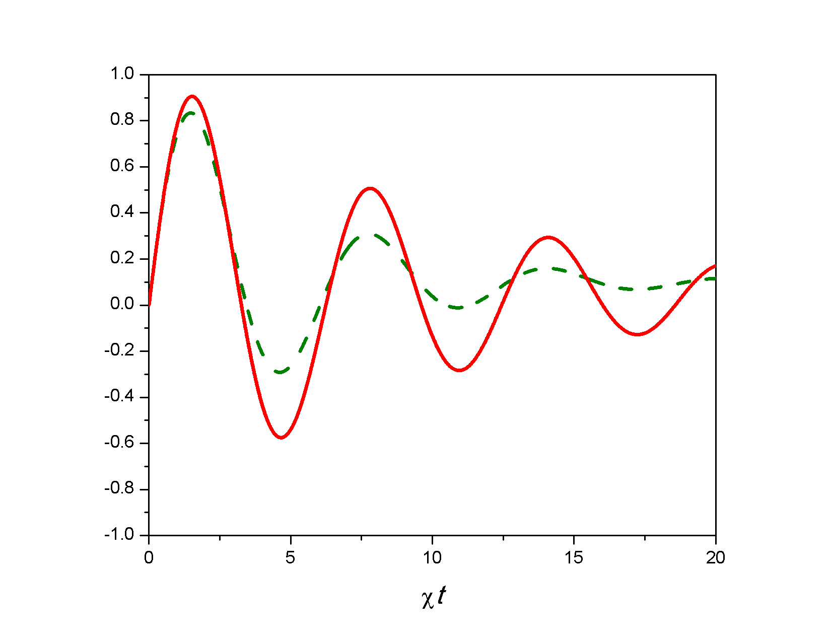
Figure 1: Plot of the function $\epsilon+e^{-2\gamma t}(\sin\chi t-\epsilon\cos\chi t)$ as a function of $\chi t$ for $\gamma=0.05$ and $\epsilon=0.05$ (solid line) and $\gamma=0.1$ and $\epsilon=0.1$ (dashed line).

$$\mu=\sqrt{\frac{\epsilon^{2}+e^{-4\gamma t}+2\epsilon\sin{\chi t}e^{-2\gamma t}}{1+\epsilon^{2}}},\qquad\tan\phi=-\frac{\epsilon+e^{-2\gamma t}(\sin\chi t-\epsilon\cos\chi t)}{\epsilon^{2}+e^{-2\gamma t}(\cos\chi t+\epsilon\sin\chi t)},$$

with $\epsilon=\gamma/\chi$ we finally obtain

$$\langle\hat{\sigma}_{x}\rangle = \frac{1}{2}\sin(2\theta)e^{-\Gamma t}\sum_{k=0}^{\infty}\mu^{n}\cos n\phi\langle k|\hat{D}^{\dagger}(\alpha)\hat{\rho}_{F}(0)\hat{D}(\alpha)|k\rangle,$$ (42)

We plot in figure 1 the numerator of $\tan\phi$, i.e. the function $\epsilon+e^{-2\gamma t}(\sin\chi t-\epsilon\cos\chi t)$ for two values of $\gamma$. Whenever this function crosses zero, $\tan\phi$ is zero. We take in particular the interaction time of the first zero, which gives $\phi=\pi$ and define $s=\frac{\mu+1}{\mu-1}$ to write

$$\langle\hat{\sigma}_{x}\rangle = \frac{1}{2}\sin(2\theta)e^{-\Gamma t}\sum_{k=0}^{\infty}\left(\frac{s+1}{s-1}\right)^{n}\langle k|\hat{D}^{\dagger}(\alpha)\hat{\rho}_{F}(0)\hat{D}(\alpha)|k\rangle,$$ (43)

or finally, comparing to equation (2)

$$\langle\hat{\sigma}_{x}\rangle = \frac{(1-s)\pi}{2}\sin(2\theta)e^{-\Gamma t}F(\alpha,s),$$ (44)

i.e., by measuring an atomic observable, namely, the atomic polarization, we can reconstruct a quasiprobability distribution function even though atomic and field decays take place.

4 Conclusions

We have solved the dispersive interaction between a quantized electromagnetic field and a decaying two-level atom in cavity subject to losses by using superoperator techniques. We have shown that even in the both decaying cases we can still obtain information about the initial cavity field by means of $s$-parametrized quasiprobability distribution functions. Due to the fact that these functions contain complete information about the state of the cavity field, we are able to determine the field state, completely. One thing to consider is the fact that an effective (dispersive) interaction produces much slower processes such that, both atomic and field decays, may be of importance.

Moreover, if we consider a very small $\theta$, i.e., the atom being mostly in the ground state with a very small contribution from the excited state, the reconstruction is still possible, as

$$\langle\hat{\sigma}_{x}\rangle\approx{(1-s)\pi}\theta e^{-\Gamma t}F(\alpha,s),$$ (45)

and, although the reconstruction would be severely diminished by such a small angle and the fact that we are considering a finite atomic decay rate, it is still possible to obtain whole information from the initial field state.

Finally note that, if we consider $\gamma=0$, i.e., an ideal cavity, $\mu=1$ [see equation (42)] and then the Wigner distribution function may be reconstructed.

References

- [1] K. Vogel and H. Risken, Phys. Rev. A 40, 2847 (1989).
- [2] U. Leonhardt, Measuring the Quantum State of Light, (Cambridge, Cambridge University Press) (1997).
- [3] S. Wallentowitz and W. Vogel, Phys. Rev. A 53, 4528 (1996).
- [4] Z. Kis, T. Kiss, J. Janszky, P.Adam, S. Wallentowitz, and W. Vogel, Phys. Rev. A 59, R39 (1999).
- [5] A. Zucchetti, W. Vogel, M. Tasche, and D.-G. Welsch, Phys. Rev. A 54, 1678 (1996).
- [6] K. Banaszek and K. Wodkiewcz, Phys. Rev. Lett. 76, 4344 (1996).
- [7] L.G. Lutterbach and L. Davidovich, Phys. Rev. Lett. 78, 2547 (1997).
- [8] H. Moya-Cessa, S.M. Dutra, J.A. Roversi, and A. Vidiella-Barranco, J. of Mod. Optics 46, 555 (1999).
- [9] H. Moya-Cessa, J.A. Roversi, S.M. Dutra, and A. Vidiella-Barranco, Phys. Rev. A 60, 4029 (1999).
- [10] U. Leonhardt and H. Paul, Phys. Rev. A 48, 4598 (1993).
- [11] U. Leonhardt and H. Paul, J. Mod. Opt. 41, 1427 (1994).
- [12] H. Moya-Cessa and P.L. Knight, Phys. Rev. A 48, 2479 (1993).
- [13] K. Husimi, Proc. Phys. Math. Soc. Jpn. 22, 264 (1940).
- [14] E.P. Wigner, Phys. Rev. 40, 749 (1932).
- [15] R.J. Glauber, Phys. Rev. A 131, 2766 (1963).
- [16] E.C.G. Sudarshan, Phys. Rev. Lett. 10, 277 (1963).
- [17] F.A.M. de Oliveira, M.S. Kim, P.L. Knight and V. Buzek, Phys. Rev. A 41, 2645 (1990).
- [18] D. Leibfried, D.M. Meekhof, B.E. King, C. Monroe, W.M. Itano, and D.J. Wineland, Phys. Rev. Lett. 77, 4281 (1996).
- [19] P. Bertet, A. Auffeves, P. Maioli, S. Osnaghi, T. Meunier, M. Brune, J.M. Raimond, and S. Haroche, Phys. Rev. Lett. 89, 200402 (2002).
- [20] R. Juarez-Amaro and H. Moya-Cessa, Phys. Rev. A 68, 023802, (2003).
- [21] T. Quang, P.L. Knight, and V. Buzek, Phys. Rev. A 44, 6092 (1991).