Very Deep Convolutional Networks for End-to-End Speech Recognition

Abstract

Sequence-to-sequence models have shown success in end-to-end speech recognition. However these models have only used shallow acoustic encoder networks. In our work, we successively train very deep convolutional networks to add more expressive power and better generalization for end-to-end ASR models. We apply network-in-network principles, batch normalization, residual connections and convolutional LSTMs to build very deep recurrent and convolutional structures. Our models exploit the spectral structure in the feature space and add computational depth without overfitting issues. We experiment with the WSJ ASR task and achieve 10.5% word error rate without any dictionary or language using a 15 layer deep network.

Index Terms—  Automatic Speech Recognition, End-to-End Speech Recognition, Very Deep Convolutional Neural Networks

1 Introduction

The sequence-to-sequence (seq2seq) model with attention [1] has recently demonstrated a promising new direction for ASR that entirely sidesteps the complicated machinery developed for classical ASR [2, 3, 4, 5, 6]. It is able to do this because it is not restricted by the classical independence assumptions of Hidden Markov Model (HMM) [7] and Connectionist Temporal Classification (CTC) [8] models. As a result, a single end-to-end model can jointly accomplish the ASR task within one single large neural network.

The foundational work on seq2seq models, however, has relied on simple neural network encoder and decoder models using recurrent models with LSTMs [4, 6] or GRUs [4]. However, their use of hierarchy in the encoders demonstrates that better encoder networks in the model should lead to better results. In this work we significantly extend the state of the art in this area by developing very deep hybrid convolutional and recurrent models, using recent developments in the vision community.

Convolutional Neural Networks (CNNs) [9] have been successfully applied to many ASR tasks [10, 11, 12]. Unlike Deep Neural Networks (DNNs) [13], CNNs explicitly exploit structural locality in the spectral feature space. CNNs use shared weight filters and pooling to give the model better spectral and temporal invariance properties, thus typically yield better generalized and more robust models compared to DNNs [14]. Recently, very deep CNNs architectures [15] have also been shown to be successful in ASR [16, 17], using more non-linearities, but fewer parameters. Such a strategy can lead to more expressive models with better generalization.

While very deep CNNs have been successfully applied to ASR, recently there have been several advancements in the computer vision community on very deep CNNs [15, 18] that have not been explored in the speech community. We explore and apply some of these techniques in our end-to-end speech model:

1. Network-in-Network (NiN) [19] increases network depth through the use of 1x1 convolutions. This allows us to increase the depth and expressive power of a network while reducing the total number of parameters that would have been needed otherwise to build such deeper models. NiN has seen great success in computer vision, building very deep models[18]. We show how to apply NiN principles in hierarchical Recurrent Neural Networks (RNNs) [20].

2. Batch Normalization (BN) [21] normalizes each layer’s inputs to reduce internal covariate shift. BN speeds up training and acts as an regularizer. BN has also seen success in end-to-end CTC models [22]. The seq2seq attention mechanism [1] has high variance in the gradient (especially from random initialization); without BN we were unable to train the deeper seq2seq models we demonstrate in this paper. We extend on previous work and show how BN can be applied to seq2seq acoustic model encoders.

3. Residual Networks (ResNets) [23] learns a residual function of the input through the usage of skip connections. ResNets allow us to train very deep networks without suffering from poor optimization or generalization which typically happen when the network is trapped at a local minima. We explore these skip connections to build deeper acoustic encoders.

4. Convolutional LSTM (ConvLSTM) [24] use convolutions to replace the inner products within the LSTM unit. ConvLSTM allows us to maintain structural representations in our cell state and output. Additionally, it allows us to add more compute to the model while reducing the number of parameters for better generalization. We show how ConvLSTMs can be beneficial and replace LSTMs.

We are driven by same motivation that led to the success of very deep networks in vision [15, 18, 21, 23] – add depth of processing using more non-linearities and expressive power, while keeping the number of parameters manageable, in effect increasing the amount of computation per parameter. In this paper, we use very deep CNN techniques to significantly improve over previous shallow seq2seq speech recognition models [4]. Our best model achieves a WER of 10.53% where our baseline acheives a WER of 14.76%. We present detailed analysis on how each technique improves the overall performance.

2 Model

In this section, we will describe the details of each component of our model.

2.1 Listen, Attend and Spell

Listen, Attend and Spell (LAS) [3] is an attention-based seq2seq model which learns to transcribe an audio sequence to a word sequence, one character at a time. Let $\mathbf{x}=(x_{1},\ldots,x_{T})$ be the input sequence of audio frames, and $\mathbf{y}=(y_{1},\ldots,y_{S})$ be the output sequence of characters. The LAS models each character output $y_{i}$ using a conditional distribution over the previously emitted characters $y_{<i}$ and the input signal $\mathrm{\mathbb{x}}$. The probability of the entire output sequence is computed using the chain rule of probabilities:

$$P(\mathbf{y}|\mathbf{x})=\prod_{i}P({y}_{i}|\mathbf{x},\mathbf{y_{<i}})$$

The LAS model consists of two sub-modules: the listener and the speller. The listener is an acoustic model encoder and the speller is an attention-based character decoder. The encoder (the $\mathrm{Listen}$ function) transforms the original signal $\mathbf{x}$ into a high level representation $\mathbf{h}=(h_{1},\ldots,h_{U})$ with $U\leq T$. The decoder (the $\mathrm{AttendAndSpell}$ function) consumes $\mathbf{h}$ and produces a probability distribution over character sequences:

$$\mathbf{h} = \mathrm{Listen}(\mathbf{x})$$ (1)

$$P(\mathbf{y}|\mathbf{x}) = \mathrm{AttendAndSpell}(\mathbf{h})$$ (2)

The $\mathrm{Listen}$ is a stacked Bidirectional Long-Short Term Memory (BLSTM) [25] network with hierarchical subsampling as described in [3]. In our work, we replace $\mathrm{Listen}$ with a network of very deep CNNs and BLSTMs. The $\mathrm{AttendAndSpell}$ is an attention-based transducer [1], which generates one character $y_{i}$ at a time:

$$s_{i} =\mathrm{DecodeRNN}([y_{i-1},c_{i-1}],s_{i-1})$$ (3)

$$c_{i} =\mathrm{AttentionContext}(s_{i},\mathbf{h})$$ (4)

$$p(y_{i}|\mathbf{x},\mathbf{y_{<i}}) =\mathrm{TokenDistribution}(s_{i},c_{i})$$ (5)

The $\mathrm{DecodeRNN}$ produces a transducer state $s_{i}$ as a function of the previously emitted token $y_{i-1}$, the previous attention context $c_{i-1}$, and the previous transducer state $s_{i-1}$. In our implementation, $\mathrm{DecodeRNN}$ is a LSTM [26] function without peephole connections.

The $\mathrm{AttentionContext}$ function generates $c_{i}$ with a content-based Multi-Layer Perceptron (MLP) attention network [1].

2.2 Network in Network

In our study, we add depth through NiN modules in the hierarchical subsampling connections between LSTM layers. We introduce a projected subsampling layer, wherein we simply concatenate two time frames to a single frame, project into a lower dimension and apply BN and ReLU non-linearity to replace the skip subsampling connections in [3]. Moreover, we further increase the depth of the network by adding more NiN 1 $\times$ 1 concolution modules inbetween each LSTM layer.

2.3 Convolutional Layers

Unlike fully connected layers, Convolutional Neural Networks (CNNs) take into account the input topology, and are designed to reduce translational variance by using weight sharing with convolutional filters. CNNs have shown improvement over traditional fully-connected deep neural networks on many ASR tasks [14, 12], we investigate the effect of convolutional layers in seq2seq models.

In a hybrid system, convolutions require the addition of context window for each frame, or a way to treat the full utterance as a single sample [17]. One advantage of the seq2seq model is that the encoder can compute gradients over an entire utterance at once. Moreover, strided convolutions are an essential element of CNNs. For LAS applying striding is also a natural way to reduce temporal resolution.

2.4 Batch Normalization

Batch normalization (BN) [21] is a technique to accelerate training and improve generalization, which is widely used in the computer vision community. Given a layer with output $\mathbf{x}$, BN is implemented by normalizing each layer’s inputs:

$$\mathrm{BN}(\mathbf{x})=\gamma\frac{\mathbf{x}-\mathrm{E}[\mathbf{x}]}{(\mathrm{Var}[\mathbf{x}]+\epsilon)^{\frac{1}{2}}}+\beta$$ (6)

where $\gamma$ and $\beta$ are learnable parameters. The standard formulation of BN for CNNs can be readily applied to DNN acoustic models and cross-entropy training. For our seq2seq model, since we construct a minibatch containing multiple utterances, we follow the sequence-wise normalization [22]. For each output channel, we compute the mean and variance statistics across all timesteps in the minibatch.

2.5 Convolutional LSTM

Fig. 1: The Convolutional LSTM (ConvLSTM) maintains spectral structural localitly in its representation. We replace the inner product of the LSTM with convolutions.

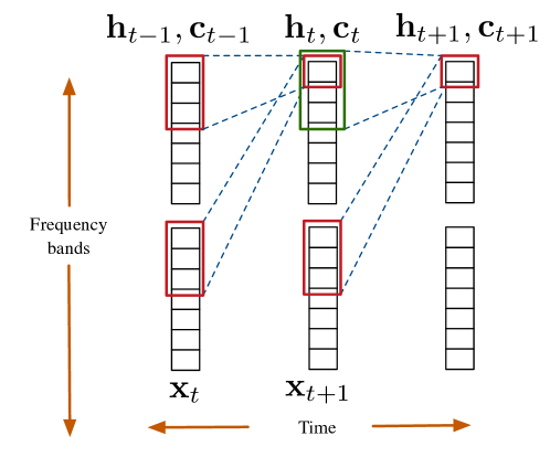
The Convolutional LSTM (ConvLSTM) was first introduced in [24]. Although the fully connected LSTM layer has proven powerful for handling temporal correlations, it cannot maintain structural locality, and is more prone to overfitting. ConvLSTM is an extension of FC-LSTM which has convolutional strucutres in both the input-to-state and state-to-state transitions:

$$\mathbf{i}_{t} =\sigma(\mathbf{W}_{xi}\ast\mathbf{x}_{t}+\mathbf{W}_{hi}\ast\mathbf{h}_{t-1}+\mathbf{b}_{i})$$

$$\mathbf{f}_{t} =\sigma(\mathbf{W}_{xf}\ast\mathbf{x}_{t}+\mathbf{W}_{hf}\ast\mathbf{h}_{t-1}+\mathbf{b}_{f})$$

$$\mathbf{c}_{t} =\mathbf{f}_{t}\odot\mathbf{c}_{t-1}+\mathbf{i}_{t}\odot\tanh(\mathbf{W}_{xc}\ast\mathbf{x}_{t}+\mathbf{W}_{hc}\ast\mathbf{h}_{t-1}+\mathbf{b}_{c})$$

$$\mathbf{o}_{t} =\sigma(\mathbf{W}_{xo}\ast\mathbf{x}_{t}+\mathbf{W}_{ho}\ast\mathbf{h}_{t-1}+\mathbf{b}_{o})$$

$$\mathbf{h}_{t} =\mathbf{o}_{t}\odot\tanh(\mathbf{c}_{t})$$ (7)

iteratively from $t=1$ to $t=T$, where $\sigma(\dot{)}$ is the logistic sigmoid function, $\mathbf{i}_{t},\mathbf{f}_{t},\mathbf{o}_{t},\mathbf{c}_{t}$ and $\mathbf{h}_{t}$ are vectors to represent values of the input gate, forget gate, output gate, cell activation, and cell output at time $t$, respectively. $\odot$ denotes element-wise product of vectors. $\mathbf{W}_{*}$ are the filter matrices connecting different gates, and $\mathbf{b}_{*}$ are the corresponding bias vectors. The key difference is that $\ast$ is now a convolution, while in a regular LSTM $\ast$ is a matrix multiplication. Figure 1 shows the internal structure of a convolutional LSTM. The state-to-state and input-to-state transitions can be achieved by a convolutional operation (here we ignore the multiple input/output channels). To ensure the attention mechanism can find the relation between encoder output and the test embedding, FC-LSTM is still necessary. However, we can use these ConvLSTMs to build deeper convolutional LSTM networks before the FC-LSTM layers. We expect this type of layer to learn better temporal representations compared to purely convolutional layers while being less prone to overfitting than FC-LSTM layers. We found bidirectional convolutional LSTMs to consistently perform better than unidirectional layers. All experiments reported in this paper used bidirectional models; here on we use convLSTM to mean bidirectional convLSTM.

2.6 Residual Network

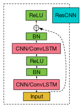
(a) ResCNN block

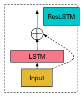
(b) ResLSTM block

Fig. 2: Residual block for different layers. ResCNN is a CNN block with CNN or ConvLSTM, Batch Normalization (BN) and ReLU non-linearities. The ResLSTM is a LSTM block with residual connections.

Deeper networks usually improve generalization and often outperform shallow networks. However, they tend to be harder to train and slower to converge when the model becomes very deep. Several architectures have been proposed recently to enable training of very deep networks [23, 27, 28, 29]. The idea behind these approaches is similar to the LSTM innovation – the introduction of linear or gated linear dependence between adjacent layers in the NN model to solve the vanishing gradient problem. In this study, we use a residual CNN/LSTM, to train deeper networks. Residual network [23] contains direct links between the lower layer outputs and the higher layer inputs. It defines a building block:

$$\mathbf{y}=\mathcal{F}(\mathbf{x},\mathbf{W}_{i})+\mathbf{x}$$ (8)

where $\mathbf{x}$ and $\mathbf{y}$ are the input and output vectors of the layers considered. The function $\mathcal{F}$ can be one or more convolutional or convLSTM layers. The residual block for different layers is illustrated in Figure 2. In our experiments, the convolutional based residual block always has a skip connection. However, for the LSTM layers we did not find skip connections necessary. All of the layers use the identity shortcut, and we did not find projection shortcuts to be helpful.

3 Experiments

We experimented with the Wall Street Journal (WSJ) ASR task. We used the standard configuration si284 dataset for training, dev93 for validation and eval92 for test evaluation. Our input features were 80 dimensional filterbanks computed every 10ms with delta and delta-delta acceleration normalized with per speaker mean and variance. The baseline $\mathrm{EncodeRNN}$ function is a 3 layer BLSTM with 256 LSTM units per-direction (or 512 total) and $4=2^{2}$ time factor reduction. The $\mathrm{DecodeRNN}$ is a 1 layer LSTM with 256 LSTM units. All the weight matrices were initialized with a uniform distribution $\mathcal{U}(-0.1,0.1)$ and bias vectors to $0$. For the convolutional model, all the filter matrices were initialized with a truncated normal distribution $\mathcal{N}(0,0.1)$, and used $32$ output channels. Gradient norm clipping to $1$ was applied, together with Gaussian weight noise $\mathcal{N}(0,0.075)$ and L2 weight decay $1\mathrm{e}{-5}$ [30]. We used ADAM with the default hyperparameters described in [31], however we decayed the learning rate from $1\mathrm{e}{-3}$ to $1\mathrm{e}{-4}$ after it converged. We used $10$ GPU workers for asynchronous SGD under the TensorFlow framework [32]. We monitor the dev93 Word Error Rate (WER) until convergence and report the corresponding eval92 WER. The models took $O(5)$ days to converge.

3.1 Acronyms for different type of layers

All the residual block follow the structure of Fig. 2. Here are the acronyms for each component we use in the following subsections:

P / 2

subsampling projection layer.

C (f $\times$ t)

convolutional layer with filter f and t under frequency and time axis.

B

batch normalization

L

bidirectional LSTM layer.

ResCNN

residual block with convolutional layer inside.

ResConvLSTM

residual block with convolutional LSTM layer inside.

3.2 Network in Network for Hierarchical Connections

We first begin by investigating the acoustic encoder depth of the baseline model without using any convolutional layers. Our baseline model follows [4] using the skip connection technique in its time reduction. The baseline L $\times$ 3 or 3 layer BLSTM acoustic encoder, model achieves a $14.76\%$ WER.

When we simply increase the acoustic model encoder depth (i.e., to depth 8), the model does not converge well and we suspect the network to be trapped in poor local minimas. By using the projection subsampling layer as discussed in Section 2.2, we improves our WER to $13.61\%$ WER or a $7.8\%$ relative gain over the baseline.

We can further increase the depth of the network by adding more NiN 1 $\times$ 1 convolution modules inbetween each LSTM layer. This improves our model’s performance further to $12.88\%$ WER or $12.7\%$ relative over the baseline. The BN layers were critical, and without them we found the model did not converge well. Table 1 summarizes the results of applying network-in-network modules in the hierarchical subsampling process.

Model	WER
L $\times$ 3	14.76
L $\times$ 8	Diverged
(L + P / 2 + B + R) $\times$ 2 + L	13.61
(L + P / 2 + B + R + C(1$\times$1) + BN + R) $\times$ 2 + L	12.88

Table 1: We build deeper encoder networks by adding NiN modules inbetween LSTM layers.

3.3 Going Deeper with Convolutions and Residual Connections

In this subsection, we extend on Section 3.2 and describe experiments in which we build deeper encoders by stacking convolutional layers and residual blocks in the acoustic encoder before the BLSTM. Unlike computer vision applications or truncated BPTT training in ASR, seq2seq models need to handle very long utterances (i.e., >2000 frames). If we simply stack a CNN before the BLSTMs, we quickly run out of GPU memory for deep models and also have excessive computation times. Our strategy to alleviate this problem is to apply striding in the first and second layer of the CNNs to reduce the time dimensionality and memory footprint.

We found no gains by simply stacking additional ResLSTM blocks even up to 8 layers. However, we do find gains if we use convolutions. If we stack 2 additional layers of 3 $\times$ 3 convolutions our model improves to 11.80% WER or 20% relative over the baseline. If we take this model and add 8 residual blocks (for a total of $(2+(8)2+5)=23$ layers in the encoder) our model further improves to $11.11\%$ WER, or a $24.7\%$ relative improvement over the baseline. We found that using 8 residual blocks a slightly outperform 4 residual blocks. Table 2 summarizes the results of these experiments.

Model	WER
L $\times$ 3	14.76
NiN (from Section 3.2)	12.88
ResLSTM $\times$ 8	15.00
(C (3 $\times$ 3) / 2) $\times$ 2 + NiN	11.80
(C (3 $\times$ 3) / 2) $\times$ 2 + ResCNN $\times$ 4 + NiN	11.30
(C (3 $\times$ 3) / 2) $\times$ 2 + ResCNN $\times$ 8 + NiN	11.11

Table 2: We build deeper encoder networks by adding convolution and residual network blocks. The NiN block equals (L + C (1x1) + B + R) $\times$ 2 + L).

3.4 Convolutional LSTM

Fig. 3: Our best model: includes two convolutional layer at the bottom and followed by four residual block and LSTM NiN block. Each residual block contains one convolutional LSTM layer and one convolutional layer.

Model	WER
L $\times$ 3	14.76
ConvLSTM $\times$ 3	24.23
(C (3$\times$3)) $\times$ 2 + ResCNN $\times$ 4 + NiN	11.30
(C (3$\times$3)) $\times$ 2 + ResConvLSTM ($3\times 1$) $\times$ 4 + NiN	10.53

Table 3: Performance of models with convolutional LSTM layers. The NiN block equals (L + C (1x1) + B + R) $\times$ 2 + L).

Model	WER
CTC (Graves et al., 2014) [33]	30.1
seq2seq (Bahdanau et al., 2016) [5]	18.0
seq2seq + deep convolutional (our work)	10.53

Table 4: Wall Street Journal test eval92 Word Error Rate (WER) results across Connectionist Temporal Classification (CTC) and Sequence-to-sequence (seq2seq) models. The models were decoded without a dictionary or language model.

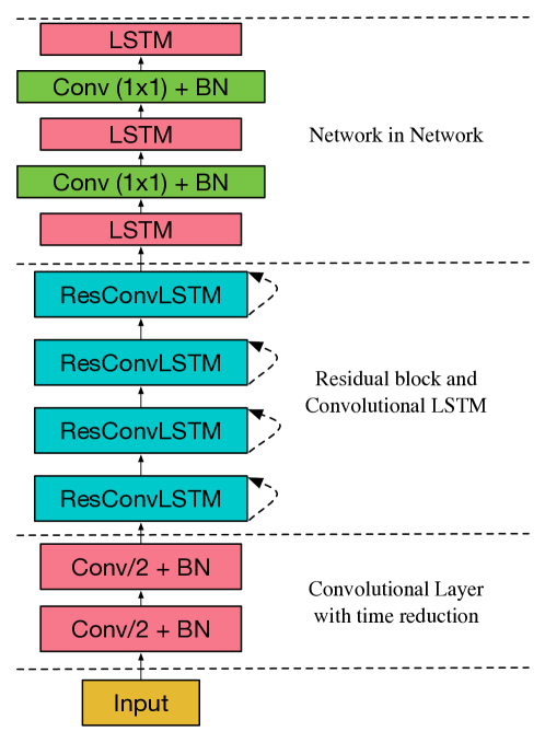
In this subsection, we investigate the effectiveness of the convolutional LSTM. Table 3 compares the effect of using convolutional LSTM layers. It can be observed that a pure ConvLSTM performs much worse than the baseline — we still need the fully connected LSTM . However, replacing the ResConv block with ResConvLSTM as shown in Figure 3 give us additional $7\%$ relative gains. In our experiments, we always use 3$\times$1 filters for ConvLSTM because the recurrent structure captures temporal information while the convolutions capture spectral structure. We conjecture that the gain is because the convolutional recurrent state maintains spectral structure and reduces overfitting.

Table 4 compares our WSJ results with other published end-to-end models. To our knowledge, the previous best reported WER on WSJ without an LM was the seq2seq model with Task Loss Estimation achieving 18.0% WER in [5]. Our baseline, also a seq2seq model, achieved 14.76% WER. Our model is different from that of [5] in that we did not use location-based priors on the attention model and we used weight noise. Our best model, shown in Figure 3, achieves a WER of 10.53%.

4 Conclusion

We explored very deep CNNs for end-to-end speech recognition. We applied Network-in-Network principles to add depth and non-linearities to hierarchical RNNs. We also applied Batch Normalization and Residual connections to build very deep convolutional towers to process the acoustic features. Finally, we also explored Convolutional LSTMs, wherein we replaced the inner product of LSTMs with convolutions to maintain spectral structure in its representation. Together, we added more expressive capacity to build a very deep model without substantially increasing the number of parameters. On the WSJ ASR task, we obtained $10.5\%$ WER without a language model, an $8.5\%$ absolute improvement over published best result [4]. While we demonstrated our results only on the seq2seq task, we believe this architecture should also significantly help CTC and other recurrent acoustic models.

5 References

References

- [1] Dzmitry Bahdanau, Kyunghyun Cho and Yoshua Bengio “Neural Machine Translation by Jointly Learning to Align and Translate” In ICLR, 2015
- [2] Jan Chorowski et al. “Attention-Based Models for Speech Recognition” In NIPS, 2015
- [3] William Chan, Navdeep Jaitly, Quoc Le and Oriol Vinyals “Listen, Attend and Spell: A Neural Network for Large Vocabulary Conversational Speech Recognition” In ICASSP, 2016
- [4] Dzmitry Bahdanau et al. “End-to-end Attention-based Large Vocabulary Speech Recognition” In ICASSP, 2016
- [5] Dzmitry Bahdanau et al. “Task Loss Estimation for Sequence Prediction” In ICLR Workshop, 2016
- [6] William Chan and Ian Lane “On Online Attention-based Speech Recognition and Joint Mandarin Character-Pinyin Training” In INTERSPEECH, 2016
- [7] Lawrence R. Rabiner “A tutorial on hidden Markov models and selected applications in speech recognition” In Proceedings of the IEEE 77, 1989, pp. 257–286
- [8] Alex Graves “Sequence Transduction with Recurrent Neural Networks” In ICML: Representation Learning Workshop, 2012
- [9] Yann LeCun, Leon Bottou, Yoshua Bengio and Patrick Haffner “Gradient-based learning applied to document recognition” In Proceedings of the IEEE 86, 1998, pp. 2278–2324
- [10] Ossama Abdel-Hamid, Li Deng and Dong Yu “Exploring Convolutional Neural Network Structures and Optimization Techniques for Speech Recognition” In INTERSPEECH, 2013
- [11] Tara Sainath, Abdel-rahman Mohamed, Brian Kingsbury and Bhuvana Ramabhadran “Deep Convolutional Neural Networks for LVCSR” In ICASSP, 2013
- [12] William Chan and Ian Lane “Deep Convolutional Neural Networks for Acoustic Modeling in Low Resource Languages” In ICASSP, 2016
- [13] Geoffrey Hinton et al. “Deep Neural Networks for Acoustic Modeling in Speech Recognition: The Shared Views of Four Research Groups” In IEEE Signal Processing Magazine, 2012
- [14] Tara Sainath et al. “Improvements to Deep Convolutional Neural Networks for LVCSR” In ASRU, 2013
- [15] Karen Simonyan and Andrew Zisserman “Very Deep Convolutional Networks for Large-Scale Image Recognition” In ICLR, 2015
- [16] Tom Sercu, Christian Puhrsch, Brian Kingsbury and Yann LeCun “Very deep multilingual convolutional neural networks for LVCSR” In ICASSP, 2016
- [17] Tom Sercu and Vaibhava Goel “Advances in Very Deep Convolutional Neural Networks for LVCSR” In INTERSPEECH, 2016
- [18] Christian Szegedy et al. “Going Deeper with Convolutions” In CVPR, 2015
- [19] Min Lin, Qiang Chen and Shuicheng Yan “Network In Network” In ICLR, 2013
- [20] Salah Hihi and Yoshua Bengio “Hierarchical Recurrent Neural Networks for Long-Term Dependencies” In NIPS, 1996
- [21] Sergey Ioffe and Christian Szegedy “Batch Normalization: Accelerating Deep Network Training by Reducing Internal Covariate Shift” In ICML, 2015
- [22] Dario Amodei et al. “Deep Speech 2: End-to-End Speech Recognition in English and Mandarin” In ICML, 2016
- [23] Kaiming He, Xiangyu Zhang, Shaoqing Ren and Jian Sun “Deep Residual Learning for Image Recognition” In CVPR, 2016
- [24] Xingjian Shi et al. “Convolutional LSTM Network: A Machine Learning Approach for Precipitation Nowcasting” In NIPS, 2015
- [25] Alex Graves, Navdeep Jaitly and Abdel-rahman Mohamed “Hybrid Speech Recognition with Bidirectional LSTM” In ASRU, 2013
- [26] Sepp Hochreiter and Jurgen Schmidhuber “Long Short-Term Memory” In Neural Computation 9.8, 1997, pp. 1735–1780
- [27] Yu Zhang et al. “Highway Long Short-Term Memory RNNs for Distant Speech Recognition” In ICASSP, 2016
- [28] Nal Kalchbrenner, Ivo Danihelka and Alex Graves “Grid long short-term memory” In ICLR, 2016
- [29] Rupesh Srivastava, Klaus Greff and Jürgen Schmidhuber “Training Very Deep Networks” In NIPS, 2015
- [30] Alex Graves “Practical Variational Inference for Neural Networks” In NIPS, 2011
- [31] Diederik Kingma and Jimmy Ba “Adam: A Method for Stochastic Optimization” In ICLR, 2015
- [32] Martín Abadi et al. “TensorFlow: Large-Scale Machine Learning on Heterogeneous Systems” Software available from tensorflow.org, 2015 URL: http://tensorflow.org/
- [33] Alex Graves and Navdeep Jaitly “Towards End-to-End Speech Recognition with Recurrent Neural Networks” In ICML, 2014