Quantum Theory of Continuum Optomechanics

Abstract

We present the basic ingredients of continuum optomechanics, i.e. the suitable extension of cavity optomechanical concepts to the interaction of photons and phonons in an extended waveguide. We introduce a real-space picture and argue which coupling terms may arise in leading order in the spatial derivatives. This picture allows us to discuss quantum noise, dissipation, and the correct boundary conditions at the waveguide entrance. The connections both to optomechanical arrays as well as to the theory of Brillouin scattering in waveguides are highlighted. We identify the ’strong coupling regime’ of continuum optomechanics that may be accessible in future experiments.

I Introduction

Cavity optomechanics aspelmeyer_cavity_2014 is a very active research area at the interface of nanophysics and quantum optics. Its aim is to exploit radiation forces to couple optical and vibrational modes in a confined geometry, with applications ranging from sensitive measurements, wavelength conversion, and squeezing all the way to fundamental questions of quantum physics. The paradigmatic cavity-optomechanical system is zero-dimensional, i.e. there is no relevant notion of spatial distance or dimensionality that would affect the dynamics in an essential way.

However, even though the vast majority of optomechanical systems rely on an optical cavity, there are a number of implementations that evade this paradigm. In particular, optomechanical effects are observed in waveguide-type structures, where both the optical field and the vibrations propagate in 1D, with the potential to uncover new classical and quantum phenomena. For example, these include waveguides fabricated on a chip rakich_giant_2012 ; van_laer_interaction_2015 as well as thin membranes suspended in hollow core fibres butsch_cw-pumped_2014 . There have also been hybrid approaches, e.g., where the light propagates along the waveguide but couples to a localized mechanical mode li_harnessing_2008 , or with acoustic waves in whispering-gallery microresonators bahl_observation_2012 ; bahl_brillouin_2013 .

Coupling light and sound inside a waveguide has long been the subject of studies on Brillouin (and Raman) scattering in fibres shen_theory_1965 ; shelby_guided_1985 ; boyd_nonlinear_2013 ; agrawal_nonlinear_2012 . This connection, between Brillouin physics and optomechanics, has recently been recognized as potentially fertile, and during the past year, first theoretical studies emphasizing this connection have emerged. The cavity-optomechanical coupling in a torus has been derived by starting from the known description of Brillouin interactions in an infinitely extended waveguide van_laer_unifying_2016 . Conversely, the Hamiltonian coupling light and sound in such waveguides has been derived starting from the microscopic optomechanical interaction laude_lagrangian_2015 ; sipe_hamiltonian_2016 ; zoubi_optomechanical_2016 ; kharel_noise_2016 , including both boundary and photoelastic terms and fully incorporate geometric and material properties of the system. These works represent important bridges between the rapidly developing field of optomechanics and the significantly more advanced field of Brillouin scattering.

Independently, the role of dimensionality has also been emphasized for several years now in another area of optomechanics: Discrete optomechanical arrays, i.e. periodic (1D or 2D) lattices of coupled optical and vibrational modes. These could be implemented in various settings, including photonic crystals safavi-naeini_two-dimensional_2014 , coupled optical disk resonators zhang_synchronization_2015 , or stacks of membranes. Recent theoretical studies have revealed their interesting properties, including the generation of photon-phonon bandstructures chang_slowing_2011 ; chen_photon_2014 ; schmidt_optomechanical_2015-1 , synchronization and nonlinear dynamics heinrich_collective_2011 , effects of long-range coupling xuereb_strong_2012 ; schmidt_optomechanical_2012 ; xuereb_reconfigurable_2014 , quantum many-body physics ludwig_quantum_2013 , and the creation of artificial gauge fields and topological transport schmidt_optomechanical_2015 ; peano_topological_2015 ; walter_dynamical_2015 .

In the present manuscript, our aim is to establish simplified foundations for “continuum optomechanics”, i.e., optomechanics in 1D waveguides without cavity modes: (i) We introduce a real-space picture and discuss how one can enumerate the possible coupling terms to leading order in spatial derivatives. (ii) We show how the continuum limit arises starting from discrete optomechanical arrays, thereby connecting Brillouin physics and these lattice structures. (iii) We include dissipation and quantum noise, deriving the quantum Langevin equations and the boundary conditions at the input of the waveguide. (iv) We identify the ’strong coupling regime’ that may be accessible in the future. (v) We provide an overview of experimentally achieved coupling parameters.

II Continuum Optomechanics in a Real-Space Formulation

The usual cavity-optomechanical interaction Hamiltonian connects the photon field $\hat{a}$ of a localized optical mode and the phonon field $\hat{b}$ of a localized vibrational mode. It is of the parametric form aspelmeyer_cavity_2014

$$-\hbar g_{0}\hat{a}^{\dagger}\hat{a}(\hat{b}+\hat{b}^{\dagger})\,.$$ (1)

Our goal is to generalize this in the most straightforward way to the case of 1D continuum fields. We will do so in in real space, using phenomenological considerations. For an evaluation of the coupling constants for particular geometries one would resort to microscopic approaches, such as those presented recently in laude_lagrangian_2015 ; sipe_hamiltonian_2016 ; zoubi_optomechanical_2016 ; sarabalis_guided_2016 . While these approaches are powerful, and necessary to design an experimental system, they are involved and rather complex as an entry point into continuum optomechanics. Therefore, a phenomenological analysis can be useful in its own right. For many purposes, the level of detail provided here will be sufficient – similar to cavity optomechanics, where the microscopic calculation of $g_{0}$ is left as a separate task. Moreover, a real-space picture is particularly useful in spatially inhomogeneous situations, such as those brought about by disorder, design, or nonlinear structure formation.

We introduce photon and phonon fields $\hat{a}(x)$ and $\hat{b}(x)$, respectively, for the waveguide geometry that we have in mind (Fig. 1). In contrast to prior treatments, we do not assume the fields to be sharply peaked around a particular wavevector laude_lagrangian_2015 ; sipe_hamiltonian_2016 ; zoubi_optomechanical_2016 ; kharel_noise_2016 . This keeps our approach general and simplifies the representation of the interacting fields, especially for situations with strongly nonlinear dynamics. For example, this apprach avoids the need to treat cascaded forward-scattering with an infinite number of photon fields wolff_cascaded_2016 . The fields are normalized such that the total photon number in the entire system would be $\int dx\,\hat{a}^{\dagger}(x)\hat{a}(x)$, and likewise for the phonons. In addition, the fields obey the usual bosonic commutation relations for a 1D field, e.g. $\left[\hat{a}(x),\hat{a}^{\dagger}(x^{\prime})\right]=\delta(x-x^{\prime})$. For a nearly monochromatic wave packet of frequency $\omega$, the energy density at position $x$ is $\hbar\omega\left\langle\hat{a}^{\dagger}(x)\hat{a}(x)\right\rangle$, and the power can be obtained by multiplying this by the group velocity. The plane-wave normal modes would be $\hat{a}(k)=\int\left(dx/\sqrt{2\pi}\right)\,e^{-ikx}\hat{a}(x)$, with $\left[\hat{a}(k),\hat{a}^{\dagger}(k^{\prime})\right]=\delta(k-k^{\prime})$.

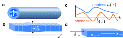
Figure 1: Continuum optomechanics. (a) Dual nanoweb structure in photonic crystal fibres; displacement field $\hat{u}(x)$ describing deflection of the membranes. (b) Nanobeam; $\hat{u}(x)$ describing longitudinal displacement. (c) Photon and phonon fields in a 1D waveguide geometry. (d) Situation at the input facet, relevant for the boundary conditions.

The normalized mechanical displacement field can be written as $\hat{u}(x)=\hat{b}(x)+\hat{b}^{\dagger}(x)$. The physical displacement at any given point will be obtained by multiplying with the mode function. As is well-known from standard cavity optomechanics, any arbitrariness arising from the mode function normalization is avoided by formulating everything in terms of $\hat{a}(x)$ and $\hat{b}(x)$, since their normalization is directly tied to the overall energy in the system.

The most obvious continuum optomechanical interaction can be written down as a direct generalization of the cavity case:

$$\hat{H}_{{\rm int}}=-\hbar\tilde{g}_{0}\int dx\,\hat{a}^{\dagger}(x)\hat{a}(x)\hat{u}(x)\,.$$ (2)

Here $\tilde{g}_{0}$ defines the continuum optomechanical coupling constant, which replaces the usual single-photon cavity-optomechanical coupling $g_{0}$. We note that $\tilde{g}_{0}$ has dimensions of frequency times the square root of length. Its meaning can be understood best in the following way: If there is a mechanical deflection $\left\langle\hat{b}\right\rangle=1/\sqrt{l}$, corresponding to 1 phonon per length $l$, then the energy of any photon is shifted by $-\hbar\tilde{g}_{0}2/\sqrt{l}$. We will comment more on the $\sqrt{l}$ dependence when we make the connection to discrete optomechanical arrays.

While Eq. (2) is a plausible ansatz, it turns out to be only a part of the full interaction. Specifically, in a real-space formulation of the continuum case, derivative terms may appear, which we will now discuss.

There are both boundary and bulk terms that contribute to the shift of optical frequency when a dielectric is deformed, as is well-known for optomechanics and has also been discussed recently in the present context sipe_hamiltonian_2016 ; zoubi_optomechanical_2016 . The boundary terms are proportional to the displacement $\hat{u}$, and as such their most natural representation is in the form of the ansatz given above, if $\hat{u}$ is chosen to represent the deflection of the boundary (more on this, see below). The bulk terms (photoelastic response), however, depend only on the spatial derivatives of the displacement field. In particular, this also involves derivatives along the longitudinal (waveguide) direction, and these terms then naturally lead to an expression

$$\hat{H}_{{\rm int}}^{++-}=-\hbar g_{0}^{++-}\int dx\,\hat{a}^{\dagger}(x)\hat{a}(x)\partial_{x}\hat{u}(x)\,.$$ (3)

We have introduced a superscript $++-$ for the coupling constant, indicating the possible presence of a derivative: $\partial_{x}\hat{u}$ changes sign if we set $\hat{u}(x)\mapsto\hat{u}(-x)$, so we associate a negative signature.

It is important to note that the shape of the Hamiltonian depends on the physical meaning of the displacement $\hat{u}$, which is to some degree a matter of definition. We have to distinguish the full vector field $\hat{\vec{u}}(\vec{r})$, which is defined unambiguously, from the reduced one-dimensional field $\hat{u}(x)$ that forms the object of our analysis. As a concrete example, consider longitudinal waves on a nanobeam. The 1D field $\hat{u}(x)$ could then be defined as the longitudinal displacement, evaluated at the beam center (see Fig. 1b, white arrow). In that case the density change, responsible for the photoelastic coupling, is proportional to $\partial_{x}\hat{u}(x)$. At the same time, a finite Poisson ratio will lead to a lateral expansion of the beam, i.e. a motion of the surface. The surface deflection will be proportional to the density change, and thus also determined by $\partial_{x}\hat{u}(x)$. However, we could have defined $\hat{u}(x)$ differently, namely to represent directly the surface deflection (Fig. 1b, black arrows). In that case, the density change would be given by $\hat{u}(x)$. Two different, equally valid definitions of $\hat{u}(x)$ would thus lead to different expressions in the Hamiltonian.

Besides the appearance of derivatives $\partial_{x}\hat{u}$, we may also encounter derivatives of the electric field. It is well-known that electromagnetic waves inside matter can also have longitudinal components, which change sign upon inversion of the propagation direction (in contrast to the transverse fields). Consequently, the electromagnetic mode functions depend on the direction of the wavevector, i.e. $\vec{E}(\vec{r})=\vec{E}_{k}(\vec{r}_{\perp})\exp(ikx)$. Upon going to our reduced 1D real-space description, this dependence on the sign of $k$ leads to terms that are the derivatives of the 1D field, since for a plane wave $\hat{a}(x)=\hat{a}e^{ikx}$ we have $\partial_{x}\hat{a}(x)=ik\hat{a}(x)$ . Any terms in the full 3D light-matter coupling that depended on the longitudinal components (that change sign with $k$) will give rise to such derivatives of the 1D fields.

In summary, the possible combinations of derivatives that can occur are listed in table 1.

Even coupling terms	Odd coupling terms
$g_{0}^{+++}\hat{a}^{\dagger}\hat{a}\hat{u}$	$g_{0}^{++-}\hat{a}^{\dagger}\hat{a}\left(\partial_{x}\hat{u}\right)$
$g_{0}^{--+}\left(\partial_{x}\hat{a}^{\dagger}\right)\left(\partial_{x}\hat{a}\right)\hat{u}$	$g_{0}^{-++}\left(\partial_{x}\hat{a}^{\dagger}\right)\hat{a}\hat{u}+{\rm h.c.}$
$g_{0}^{-+-}(\partial_{x}\hat{a}^{\dagger})\hat{a}(\partial_{x}\hat{u})+{\rm h.c.}$	$g_{0}^{---}\left(\partial_{x}\hat{a}^{\dagger}\right)\left(\partial_{x}\hat{a}\right)\left(\partial_{x}\hat{u}\right)$

Table 1: Possible coupling terms (to leading order in the derivatives) for continuum optomechanics, formulated in real-space. The Hamiltonian is of the form $-\hbar\int dx(...)$, with the integrand $(...)$ containing one or more terms displayed here.

This is a complete list of the coupling terms that can arise in a minimalistic model of continuum optomechanics. The simplest choice, introduced in the beginning, would be identified as $\tilde{g}_{0}=g_{0}^{+++}$. Even and odd terms cannot be present simultaneously, unless inversion symmetry is broken. As remarked above, one can choose the definition of the 1D field $\hat{u}(x)$ to select either the “even” or the “odd” representation. Note that the constants have different physical dimensions (e.g. $g_{0}^{++-}$ is of dimensions $m^{3/2}{\rm Hz}$).

Interaction terms with derivatives would also arise by starting from the microscopic theory, keeping the dispersion ($k$-dependence) of the coupling, and translating from $k$-space into real space. In general, this would yield derivatives of any order. Here, our aim was to keep the leading terms. These are sufficient to retain a qualitatively important feature: A model based on Eq. (2) would predict that the forward- and backward-scattering amplitudes are equal (set by the single coupling constant in such a model). In reality, that is not the case, and this fact is taken into account properly by considering the derivatives.

Is our list complete? To answer this, let us discuss the “even” sector only, without loss of generality. In this sector, we went up to second order in the derivatives, keeping terms such as $\left(\partial_{x}\hat{a}^{\dagger}\right)\hat{a}\left(\partial_{x}\hat{u}\right)$. Why did we not consider second derivatives of individual fields, like $\hat{a}^{\dagger}\hat{a}\left(\partial_{x}^{2}\hat{u}\right)$? The answer is that these can indeed be present. However, a simple integration by parts will transform those terms into a combination of the terms that we already listed.

Beyond the interaction, the Hamiltonian contains the unperturbed energy of the photons, $\hat{H}_{a}=\int dk\,\hbar\omega(k)\hat{a}^{\dagger}(k)\hat{a}(k)\,,$ and likewise $\hat{H}_{b}$ for the phonons with their dispersion $\Omega(k)$. In real space, the same term could be written as $\hat{H}_{a}=\hbar\int dx\,\hat{a}^{\dagger}(x)\omega(-i\partial_{x})\hat{a}(x)\,,$ where $\omega(-i\partial_{x})$ applied to $e^{ikx}$ will reproduce $\omega(k)$.

The resulting coupled continuum optomechanical Heisenberg equations of motion take the form:

$$\partial_{t}\hat{a} = -i\omega(-i\partial_{x})\hat{a}+i\tilde{g}_{0}\hat{a}(\hat{b}+\hat{b}^{\dagger})\,$$ (4)

$$\partial_{t}\hat{b} = -i\Omega(-i\partial_{x})\hat{b}+i\tilde{g}_{0}\hat{a}^{\dagger}\hat{a}\,.$$ (5)

Here, eq. (4) and (5) are expressed with the simple interaction. More generally, the interaction may be comprised of a linear combination of terms in Table I. For example, the term $i\tilde{g}_{0}\hat{a}(\hat{b}+\hat{b}^{\dagger})$ in Eq. (4) becomes

$$ig_{0}^{+++}\hat{a}\hat{u}-ig_{0}^{--+}\partial_{x}(\hat{u}\partial_{x}\hat{a})$$

$$-ig_{0}^{-+-}\partial_{x}(\hat{a}\partial_{x}u)+ig_{0}^{-+-*}\left(\partial_{x}\hat{a}\right)\left(\partial_{x}\hat{u}\right)$$ (6)

when even couplings are considered. Likewise, term $i\tilde{g}_{0}\hat{a}^{\dagger}\hat{a}$ of Eq. (5) becomes

$$ig_{0}^{+++}\hat{a}^{\dagger}\hat{a}+ig_{0}^{--+}(\partial_{x}\hat{a}^{\dagger})(\partial_{x}\hat{a})$$

$$-ig_{0}^{-+-}\partial_{x}((\partial_{x}\hat{a}^{\dagger})\hat{a})-ig_{0}^{-+-*}\partial_{x}(\hat{a}^{\dagger}(\partial_{x}\hat{a}))$$ (7)

The real-space formulation developed here, with the complete list of interactions derived above, will be especially powerful for considering the effects of nonlinearities and of spatial inhomogeneities (whether due to disorder or structure formation). No assumptions about the fields peaking around a certain wavevector have been employed, nor are we required to introduce a multitude of photon fields for cases like forward scattering. The classical version of these nonlinear equations can readily be solved by using split-step Fourier techniques.

III Dissipation and Quantum Noise

To discuss the dissipation and the associated quantum and thermal noise, we employ the well-known input-output formalism and adapt it suitably to the continuum case. If we assume the photon loss rate to be $\kappa$, then the equation of motion contains additional terms

$$\partial_{t}\hat{a}(x,t)=\ldots-\frac{\kappa}{2}\hat{a}(x,t)+\sqrt{\kappa}\hat{a}_{{\rm in}}(x,t)\,,$$ (8)

where the vacuum noise field $\hat{a}_{{\rm in}}$ obeys the commutation relation $\left[\!\right.\hat{a}_{{\rm in}}(x,t),\hat{a}_{{\rm in}}^{\dagger}(x^{\prime},t^{\prime})\left.\!\right]=\delta(x-x^{\prime})\delta(t-t^{\prime})$ and has the correlators $\left<\!\right.\hat{a}_{{\rm in}}(x,t)\hat{a}_{{\rm in}}^{\dagger}(x^{\prime},t^{\prime})\left.\!\right>=\delta(x-x^{\prime})\delta(t-t^{\prime})$ and $\left<\!\right.\hat{a}_{{\rm in}}^{\dagger}(x^{\prime},t^{\prime})\hat{a}_{{\rm in}}(x,t)\left.\!\right>=0$. These ensure that the commutator of $\hat{a}$ is preserved, i.e. the vacuum noise is constantly being replenished to offset the losses.

The mechanical field can be treated likewise, with a damping rate $\Gamma$ in place of $\kappa$, and with the additional contribution of thermal noise: $\left<\!\right.\hat{b}_{{\rm in}}(x,t)\hat{b}_{{\rm in}}^{\dagger}(x^{\prime},t^{\prime})\left.\!\right>=(\bar{n}_{{\rm th}}+1)\delta(x-x^{\prime})\delta(t-t^{\prime})$ and $\left<\!\right.\hat{b}_{{\rm in}}^{\dagger}(x^{\prime},t^{\prime})\hat{b}_{{\rm in}}(x,t)\left.\!\right>=\bar{n}_{{\rm th}}\delta(x-x^{\prime})\delta(t-t^{\prime})$. Here $\bar{n}_{{\rm th}}=(\exp(\hbar\Omega/k_{B}T)-1)^{-1}$ is the Bose occupation at temperature $T$. For simplicity, we assume that this can be evaluated at some fixed frequency $\Omega$, since the phonon dispersion $\Omega(k)$ is usually nearly flat in the most important applications.

IV Boundary conditions

We have now collected all the ingredients for continuum optomechanics, except the driving and the boundary conditions. A laser injecting light of amplitude $\alpha_{{\rm in}}$ at point $x$ would be described by an additional term $\sqrt{\kappa_{{\rm ex}}}\alpha_{{\rm in}}(x,t)$ in the equations of motion, with $\alpha_{{\rm in}}(x,t)=\alpha_{{\rm in}}(x)e^{-i\omega_{L}t}$ for a continuous wave excitation. Here $\kappa_{{\rm ex}}$ is the coupling to the field mode that is populated by the laser photons, and $\hbar\omega_{L}\left|\alpha_{{\rm in}}(x,t)\right|^{2}$ would be the power per unit length impinging on the waveguide at position x. This description is appropriate for illumination from the side, which is feasible (and analogous to standard cavity optomechanis) but atypical in experiments.

More commonly, light is injected at the waveguide entrance. In that case, we consider a half-infinite system, starting at $x=0$ and extending to the right (Fig. 1d). The boundary at $x=0$ must be such that incoming waves (including the quantum vacuum noise) are perfectly launched into the waveguide as right-going waves, while left-moving waves exit without reflection. For the simplest case of a constant photon velocity $c$, we need to prescribe the right-going amplitude at $x=0$,

$$\partial_{t}\hat{a}(0,t)-c\partial_{x}\hat{a}(0,t)=-\sqrt{\frac{2}{c}}\partial_{t}(\alpha_{{\rm in}}(t)+\hat{a}_{{\rm in}}(t))\,,$$ (9)

where the ingoing quantum noise has the correlator

$$\left\langle\hat{a}_{{\rm in}}(t)\hat{a}_{{\rm in}}^{\dagger}(0)\right\rangle=\delta(t)$$ (10)

while $\left\langle\hat{a}_{{\rm in}}^{\dagger}(t)\hat{a}_{{\rm in}}(0)\right\rangle$ vanishes. Eq. (9) is valid also in the presence of dissipation. The solution of the free wave equation $\partial_{t}^{2}\hat{a}-c^{2}\partial_{x}^{2}\hat{a}=0$ with the boundary condition (9) is

$$\hat{a}(x,t)=\hat{a}_{\rightarrow}(x-ct)+\hat{a}_{\leftarrow}(x+ct)$$ (11)

where the right-moving field is set by $\hat{a}_{{\rm in}}(t)$:

$$\hat{a}_{\rightarrow}(x)=\hat{a}_{{\rm in}}(x/c)/\sqrt{2c}$$ (12)

The left-moving field is an independent fluctuating field. The correlator of the right-movers is

$$\left\langle\hat{a}_{\rightarrow}(x)\hat{a}_{\rightarrow}^{\dagger}(x^{\prime})\right\rangle = \frac{1}{2c}\left\langle\hat{a}_{{\rm in}}(x/c)\hat{a}_{{\rm in}}^{\dagger}(x^{\prime}/c)\right\rangle$$

$$= \frac{1}{2c}\delta(\frac{x-x^{\prime}}{c})=\frac{1}{2}\delta(x-x^{\prime})$$

and the same result holds for the left-movers, such that the full equal-time correlator of the $\hat{a}(x)$ field is set by $\delta(x-x^{\prime})$.

V Rotating Frame and Linearized Description

We can switch to a rotating frame, $\hat{a}^{{\rm old}}(x,t)=\hat{a}^{{\rm new}}(x,t)\cdot e^{i(k_{L}x-\omega_{L}t)}$, where $\omega_{L}=\omega(k_{L})$ is the laser frequency. For brevity, we drop the superscript ’new’, i.e. all $\hat{a}$ are now understood to be in the rotating frame. We then have, in the photon equation of motion, after employing $\omega(-i\partial_{x})e^{ik_{L}x}=e^{ik_{L}x}\omega(k_{L}-i\partial_{x})$:

$$\partial_{t}\hat{a}=-i\tilde{\omega}(-i\partial_{x})\hat{a}+\ldots\,$$ (13)

For brevity, we define $\tilde{\omega}(-i\partial_{x})=\omega(k_{L}-i\partial_{x})-\omega_{L}$. If only modes close to $k_{L}$ are present, this may be expanded using the group velocity $v=d\omega(k_{L})/dk$:

$$\partial_{t}\hat{a}=-v\partial_{x}\hat{a}+\ldots\,.$$ (14)

The equation for the phonon field remains unaffected by this change.

We can linearize the equations in the standard way (see Supplementary Material), setting $\beta(x)=\left\langle\hat{b}(x)\right\rangle$ and $\alpha(x)=\left\langle\hat{a}(x)\right\rangle$ for the steady-state solution, and $\delta\hat{b}=\hat{b}-\beta$ and $\delta\hat{a}=\hat{a}-\alpha$ for the fluctuations. Then we obtain, for the simplest interaction term:

$$\partial_{t}\delta\hat{a} = -i\tilde{\omega}(-i\partial_{x})\delta\hat{a}+i\tilde{g}(x)(\delta\hat{b}+\delta\hat{b}^{\dagger})+i\tilde{g}_{\beta}(x)\delta\hat{a}+\ldots$$ (15)

$$\partial_{t}\delta\hat{b} = -i\Omega(-i\partial_{x})\delta\hat{b}+i(\tilde{g}(x)\delta\hat{a}(x)^{\dagger}+\tilde{g}^{*}(x)\delta\hat{a}(x))+\ldots$$ (16)

Here we introduced the linearized coupling $\tilde{g}(x)\equiv\tilde{g}_{0}\alpha(x)$, as well as the shift $\tilde{g}_{\beta}(x)\equiv\tilde{g}_{0}(\beta(x)+\beta^{*}(x))$. The omitted terms ($\ldots$) in Eqs. (15) and (16) contain the dissipation and fluctuations, in the same form as above (only with $\hat{a}\mapsto\delta\hat{a}$, and the same for the phonons). The boundary conditions for the fluctuations $\delta\hat{a}$ do not contain any laser driving any more; i.e. we would have Eq. (9) for $\delta\hat{a}$, but without the laser amplitude $\alpha_{{\rm in}}$.

VI Continuum limit for optomechanical arrays

In an optomechanical array, discrete localized optical and vibrational modes are coupled to each other via the optomechanical interaction $-\hbar g_{0}\hat{a}_{j}^{\dagger}\hat{a}_{j}(\hat{b}_{j}+\hat{b}_{j}^{\dagger})$, see Fig. 2. In addition, the photon and phonon modes $\hat{a}_{j}$ and $\hat{b}_{j}$ are coupled by tunneling between neighboring sites. For the photons, in a 1D array, this is described by the tight-binding Hamiltonian $-\hbar\sum_{j,l}J_{l}\hat{a}_{j+l}^{\dagger}\hat{a}_{j}+{\rm h.c.}$. Here $J_{l}$ is the tunnel coupling connecting any two sites $j$ and $j+l$. The resulting dispersion relation for the optical tight-binding band is $\omega(k)=-\sum_{l}e^{-ikl\delta x}J_{l}$, where we already introduced the lattice constant $\delta x$. For the phonons, an analogous Hamiltonian holds, with a coupling constant $K_{l}$ and a resulting phononic band $\Omega(k)$.

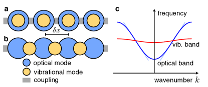
Figure 2: (a) Schematic of a 1D optomechanical array, with discrete localized optical and vibrational modes that are coupled locally. (b) An alternative situation, where phonons couple to photon tunneling between sites. (c) Bare bandstructure for phonons (red) and photons (blue; shifted by an offset that is determined by the pump laser frequency, using a rotating frame). The plot is shown for zero optomechanical coupling.

The continuum theory will be a faithful approximation if only modes of sufficiently long wavelengths (many lattice spacings) are excited. The properly normalized way to identify localized modes with the continuum fields is

$$\hat{a}_{j}=\hat{a}(j\delta x)\sqrt{\delta x},\,\hat{b}_{j}=\hat{b}(j\delta x)\sqrt{\delta x}\,.$$ (17)

This ensures the validity of the commutator relations such as $\left[\hat{a}(x),\hat{a}^{\dagger}(x^{\prime})\right]=\delta(x-x^{\prime})$. We then obtain

$$\hat{H}_{{\rm int}}^{{\rm array}} = -\hbar g_{0}\sum_{j}\hat{a}_{j}^{\dagger}\hat{a}_{j}(\hat{b}_{j}+\hat{b}_{j}^{\dagger})$$ (18)

$$\approx \hat{H}_{{\rm int}}^{{\rm cont}}\,.$$

Here $\hat{H}_{{\rm int}}^{{\rm cont}}$ is the continuum version of Eq. (2). For this simple local interaction, none of the ’derivative-terms’ appears. The present approximation holds when the Hamiltonian acts on states where only long-wavelength modes are excited. We can now relate the coupling constants for the continuum and the discrete model:

$$\tilde{g}_{0}=g_{0}\sqrt{\delta x}\,.$$ (19)

In taking the proper continuum limit, $\tilde{g}_{0}$ has to be kept fixed, i.e. $g_{0}\sim 1/\sqrt{\delta x}$ as $\delta x\rightarrow 0$. This is the expected physical behaviour, since $g_{0}\sim x_{{\rm ZPF}}$, where $x_{{\rm ZPF}}=\sqrt{\hbar/(2m\Omega)}$ is the size of the mechanical zero-point fluctuations of a discrete mechanical mode. If this mode represents a piece of length $\delta x$ in a continuous waveguide, its mass scales as $m=\delta x\cdot\rho$ [with $\rho$ the mass density], such that $g_{0}$ grows in the manner discussed above when $\delta x$ is sent to zero. Note that the continuum limit also means keeping $\omega(k)$ and $\Omega(k)$ fixed in the relevant wavelength range.

One can now also confirm that our treatment of quantum noise and dissipation corresponds to the input-output formalism applied to the discrete modes. For such modes, we would have $\dot{\hat{a}}_{j}=\ldots-\frac{\kappa}{2}\hat{a}_{j}+\sqrt{\kappa}\hat{a}_{j,{\rm in}}(t)$, with $\left\langle\hat{a}_{j,{\rm in}}(t)\hat{a}_{j^{\prime},{\rm in}}^{\dagger}(0)\right\rangle=\delta_{j,j^{\prime}}\delta(t)$ and $\left[\hat{a}_{j,{\rm in}},\hat{a}_{j^{\prime},{\rm in}}^{\dagger}\right]=\delta_{j,j^{\prime}}$. Setting $\hat{a}_{j,{\rm in}}(t)=\sqrt{\delta x}\hat{a}_{{\rm in}}(j\delta x,t)$, this turns into the continuum expressions given above.

We turn back to the optomechanical interaction in the array. So far, we had assumed a local interaction of the type $-\hbar g_{0}\hat{a}^{\dagger}\hat{a}(\hat{b}_{j}^{\dagger}+\hat{b}_{j})$. However, it is equally possible to have an interaction that creates phononic excitations during the photon tunneling process: $-\hbar g_{0}(\hat{a}_{j+1}^{\dagger}\hat{a}_{j}+{\rm h.c.})\hat{u}_{j}$, where $\hat{u}_{j}\equiv\hat{b}_{j}+\hat{b}_{j}^{\dagger}$ describes the displacement of a mode attached to the link between the sites $j$ and $j+1$; see Fig. 2b. It turns out that such a coupling gives rise to ’derivative’ terms in the continuum model, see the Supplementary Material.

VII Elementary processes for a single optical branch

We briefly connect the real-space and $k$-space pictures to review the elementary scattering processes. Translating the couplings in table 1 to $k$-space, we arrive at the substitutions $\hat{a}(x)\mapsto\hat{a}_{k}$, $\hat{a}^{\dagger}(x)\mapsto\hat{a}_{k+q}^{\dagger}$ and $\hat{u}(x)\mapsto\hat{u}_{q}$, with $\hat{u}_{q}=\hat{b}_{q}+\hat{b}_{-q}^{\dagger}$. In addition, $\partial_{x}\hat{a}\mapsto ik\hat{a}_{k}$, $\partial_{x}\hat{a}^{\dagger}\mapsto-i(k+q)\hat{a}_{k+q}^{\dagger}$, and $\partial_{x}\hat{u}\mapsto iq\hat{u}_{q}$. This yields the following amplitude (for the example of the “even” sector) in front of the resulting term $\hat{a}_{k+q}^{\dagger}\hat{a}_{k}\hat{u}_{q}$ in the Hamiltonian:

$$-\hbar\left\{g_{0}^{+++}+g_{0}^{--+}(k+q)k+g_{0}^{-+-}(k+q)q-g_{0}^{-+-*}kq\right\}$$ (20)

We can now specifically distinguish the amplitudes for forward-scattering ($q\approx 0$):

$$g_{0F}=g_{0}^{+++}+g_{0}^{--+}k^{2}$$ (21)

and backward-scattering ($q\approx-2k$):

$$g_{0B}=g_{0}^{+++}-k^{2}g_{0}^{--+}+2k^{2}(g_{0}^{-+-}+g_{0}^{-+-*})\,.$$ (22)

Clearly it was important to keep more than the simplest interaction term $g_{0}^{+++}$ in real-space to allow that these amplitudes are different.

If only forward-scattering is considered, the situation is significantly different from standard cavity optomechanics. The reason is that the cavity allows us to introduce an asymmetry between Stokes and anti-Stokes processes. This is absent here in forward-scattering, where phonons of wavenumber $q$ can be emitted and absorbed equally likely, scattering laser photons into a comb kang_tightly_2009 ; butsch_cw-pumped_2014 ; koehler_resolving_2016 ; wolff_cascaded_2016 of sidebands $\omega_{L}\pm n\Omega$ with $\Omega=\Omega(q)$. Because of this, basic phenomena in cavity optomechanics, like cooling or state transfer, do not translate to the forward scattering case with a single optical branch; these operation require asymmetry between Stokes and anti-Stokes coupling processes. Dispersive symmetry breaking is seldom accomplished in this geometry, as typical propagation lengths are not adequate to resolve the wavevector difference between Stokes and anti-Stokes phonon modes.

In backward scattering, the situation is different, since either phonons of wavenumber $q\cong 2k_{L}$ are emitted (Stokes) or those of wavenumber $q\cong-2k_{L}$ are absorbed (anti-Stokes). This can result in cooling of $-2k_{L}$ phonons and amplification of $+2k_{L}$ phonons. The latter process amounts to stimulated backward Brillouin scattering, amplifying any counterpropagating beam.

VIII Multiple optical branches

The useful Stokes/anti-Stokes asymmetry can be re-introduced into forward scattering by considering multiple optical branches. These might be different transverse optical modes. In that case, the (simplest) interaction is

$$-\hbar\sum_{j,l}\int dx\,\tilde{g}_{0}(j,l)\hat{a}_{j}^{\dagger}(x)\hat{a}_{l}(x)(\hat{b}(x)+\hat{b}^{\dagger}(x))\,.$$ (23)

Here $\tilde{g}_{0}(j,l)$ describes the bare coupling for scattering from branch $l$ to $j$, with $\tilde{g}_{0}^{*}(l,j)=\tilde{g}_{0}(j,l)$, and $[\hat{a}_{j}(x),\hat{a}_{l}^{\dagger}(x^{\prime})]=\delta_{jl}\delta(x-x^{\prime})$. Analogous expressions can be written down for the other interactions of table 1.

For the case of two branches, there will be forward-scattering of photons $k_{L}\mapsto k_{L}+q$ between the branches, by either absorbing a phonon of wavenumber $q$ or emitting one of wavenumber $-q$. In the linearized Hamiltonian, the inter-branch scattering process is described by

$$-\hbar\int dx\,(\tilde{g}_{21}(x)\delta\hat{a}_{2}^{\dagger}(x)+{\rm h.c.})(\delta\hat{b}(x)+\delta\hat{b}^{\dagger}(x))\,,$$ (24)

with $\tilde{g}_{21}(x)=\tilde{g}_{21}e^{ik_{L}x}$, where $\tilde{g}_{21}=\tilde{g}_{0}(2,1)\alpha_{1}$. In momentum space, this turns into

$$-\hbar\int dq\,\tilde{g}_{21}\delta\hat{a}_{2}[k_{L}+q]^{\dagger}(\delta\hat{b}[q]+\delta\hat{b}[-q]^{\dagger})+{\rm h.c.}$$ (25)

IX Interband scattering: Weak coupling

We first treat the weak coupling limit for scattering between different optical bands, which has been discussed widely in the literature and is known under various names such as stimulated Brillouin scattering (SBS) or stimulated Raman-like scattering (see Suppl. Material for a discussion of naming conventions). It is a widely studied regime of continuum optomechanical coupling, with a long history in the context of nonlinear optics chiao_stimulated_1964 ; shen_theory_1965 ; boyd_nonlinear_2013 ; agrawal_nonlinear_2012 . The phonon fields are assumed to have far shorter decay lengths than the optical waves, which is frequently satisfied by experimental systems. In this limit, the nonlinear optical susceptibility induced by optomechanics can be approximated as local, greatly simplifying the spatio-temporal dynamics. For clarity, we term this regime the ’Brillouin-limit’.

To connect our continuum optomechanical framework with Brillouin or Raman interactions, we start from Eq. (24), for two optical branches. Just as in Eqs. (13) and (14), we introduce rotating frames and linearize the dispersion relations. Then, we obtain:

$$\partial_{x}\left\langle\delta\hat{a}_{2}\right\rangle = i(\tilde{g}_{12}/v_{2})\left\langle\delta\hat{b}^{\dagger}\right\rangle-(\gamma_{2}/2)\left\langle\delta\hat{a}_{2}\right\rangle,$$ (26)

$$\partial_{x}\left\langle\delta\hat{b}\right\rangle = i(\tilde{g}_{12}/v_{b})\left\langle\delta\hat{a}_{2}^{\dagger}\right\rangle-(\gamma_{b}/2)\left\langle\delta\hat{b}\right\rangle.$$ (27)

Here, $\gamma_{2}\equiv\kappa_{2}/v_{2}$ and $\gamma_{b}\equiv\Gamma/v_{b}$ represent the spatial power decay rate of the photon (phonon) fields, i.e. the inverse decay length. Since the spatial decay rate of sound ($\gamma_{b}$) is typically much larger than that of light ($\gamma_{2}$), the phonon field is generated locally: $\partial_{x}\left\langle\delta\hat{b}\right\rangle\approx 0$. This allows to express the mechanical amplitude in terms of the light field, which yields:

$$\partial_{x}\left\langle\delta\hat{a}_{2}\right\rangle = \frac{|\tilde{g}_{12}|^{2}}{v_{1}\Gamma}\left\langle\delta\hat{a}_{2}\right\rangle-(\gamma_{2}/2)\left\langle\delta\hat{a}_{2}\right\rangle,$$ (28)

We can now cast this result in terms of traveling-wave optical powers $P_{1}$ and $P_{2}$, with $P_{1}=\hbar\omega_{1}v_{1}\left|\alpha_{1}\right|^{2}$, $P_{2}\cong\hbar\omega_{2}v_{2}\left|\left\langle\delta\hat{a}_{2}\right\rangle\right|^{2}$, and $P_{b}\cong\hbar\Omega v_{b}\left|\left\langle\delta\hat{b}\right\rangle\right|^{2}$. Here we assumed the small signal limit, i.e. $\alpha_{2}=0$, $\beta=0$, and $\alpha_{1}$ is large. We see that $P_{2}$ is exponentially amplified according to

$$\frac{\partial P_{2}}{\partial x} = G_{B}P_{1}P_{2}-\gamma_{2}P_{2},$$ (29)

where $G_{B}\equiv 4|\tilde{g}_{o}({1,2})|^{2}/(v_{1}v_{2}\Gamma\hbar\omega_{1})$ is the Brillouin gain coefficient agrawal_nonlinear_2012 ; rakich_giant_2012 . For alternative derivations in the context of nonlinear optics and Brillouin photonics, see Refs. agrawal_nonlinear_2012 ; boyd_nonlinear_2013 ; for discussion of the induced nonlinear optical susceptibility see Suppl. Material. This relationship between $G_{B}$ and $\tilde{g}_{o}({1,2})$ permits us to leverage established methods for calculation of the optomechanical coupling in both translationally invariant rakich_giant_2012 ; qiu_stimulated_2013 ; wolff_stimulated_2015 ; sipe_hamiltonian_2016 and periodic qiu_stimulated_2012 nano-optomechanical systems. In the Brilloin limit, a range of complex spatio-temporal phenomena have been studied agrawal_nonlinear_2012 ; boyd_nonlinear_2013 .

X Strong coupling in the ’Coherent-Phonon Limit’

The case opposite to the ’Brillouin limit’, that we just discussed, is the situation of a large phonon coherence length. This might be termed the ’coherent phonon limit’. In this much less explored limit, a large variety of interesting classical and quantum phenomena can be expected to appear, as the system acquires a much higher degree of coherence and nonlocality. Quantum states can then be swapped between the light field and the phonon field, which can lead to applications like opto-acoustic data storage in a fibre zhu_stored_2007 . We now consider the situation where creation of a photon in the second branch is accompanied by absorption of a phonon, instead of the emission that would lead to amplification. This leads to a modified version of Eqs. (26) and (27):

$$\partial_{x}\left\langle\delta\hat{a}_{2}\right\rangle = i(\tilde{g}_{12}/v_{2})\left\langle\delta\hat{b}\right\rangle-(\gamma_{2}/2)\left\langle\delta\hat{a}_{2}\right\rangle,$$ (30)

$$\partial_{x}\left\langle\delta\hat{b}\right\rangle = i(\tilde{g}_{12}^{*}/v_{b})\left\langle\delta\hat{a}_{2}\right\rangle-(\gamma_{b}/2)\left\langle\delta\hat{b}\right\rangle.$$ (31)

That can be recast as a matrix equation

$$\partial_{x}\phi=M\phi\,,$$ (32)

where the vector $\phi$ contains the fields, $\phi=\left(\left\langle\delta\hat{a}_{2}\right\rangle,\left\langle\delta\hat{b}\right\rangle\right){}^{T}$, and

$$M=\left(\begin{array}[]{cc}-\gamma_{2}/2&i\tilde{g}_{12}/v_{2}\\ i\tilde{g}_{12}^{*}/v_{b}&-\gamma_{b}/2\end{array}\right)\,.$$ (33)

This is a non-Hermitian matrix that can be diagonalized to obtain the spatial evolution $\phi\sim e^{\lambda x}$. We find the eigenvalues

$$\lambda_{\pm}=\frac{1}{2}\left[-\bar{\gamma}\pm\sqrt{D}\right]\,,$$ (34)

where $\bar{\gamma}=(\gamma_{2}+\gamma_{b})/2$ is the average spatial decay rate, and $D=[(\gamma_{2}-\gamma_{b})/2]^{2}-4\left|\tilde{g}_{12}\right|^{2}/v_{2}v_{b}$. A distinct oscillatory regime is reached when $D<0$, i.e.

$$\left|\tilde{g}_{12}\right|>\sqrt{v_{2}v_{b}}\frac{\left|\gamma_{2}-\gamma_{b}\right|}{4}\,.$$ (35)

In that case, the eigenvalues attain an imaginary part, and the spatial evolution becomes oscillatory. Interestingly, this sharp threshold only depends on the difference of spatial decay rates. In principle, therefore, in an unconventional system where $\gamma_{2}$ and $\gamma_{b}$ are of the same order, this condition is much easier to fulfill than when having to compare $\left|\tilde{g}_{12}\right|$ against the total decay rate. Nevertheless, in order for the oscillations to be observed in practice, in addition the decay length should be larger than the period of oscillations. This will be true when $\left|{\rm Re}\lambda\right|\ll\left|{\rm Im}\lambda\right|$, which can be approximated as

$$\left|\tilde{g}_{12}\right|\gg\sqrt{v_{2}v_{b}}\bar{\gamma}/2\,.$$ (36)

We will term this the “strong coupling regime” for continuum optomechanics. It is in spirit similar to the strong coupling regime of cavity optomechanics aspelmeyer_cavity_2014 , although the dependence on the velocities introduces a new element. If this more demanding condition (36) is fulfilled, then the coupling is also automatically larger than the threshold (35) given above.

To interpret this condition, note that usually $\bar{\gamma}$ is dominated by the phonon decay $\gamma_{b}=\Gamma/v_{b}$. In that case, we could also write $\left|\tilde{g}_{12}\right|\gg\sqrt{v_{2}/v_{b}}\Gamma/4$. This shows that, at a fixed phonon decay rate $\Gamma$, smaller phonon velocities make the strong coupling regime harder to reach.

XI Experimental Overview

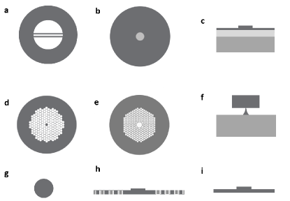
Figure 3: Overview of experimental systems including: (a) Nanoweb fibre butsch_optomechanical_2012 ; (b) Step-index fibre abedin_observation_2005 ; behunin_long-lived_2015 ; (c) Ridge waveguide pant_-chip_2010 ; (d) Crystal fibre kang_tightly_2009 ; beugnot_guided_2007 ; zhong_depolarized_2015 ; (e) Hollow core photonic crystal fiber zhong_depolarized_2015 ; renninger_guided-wave_2016 ; renninger_nonlinear_2016 ; renninger_forward_2016-1 ; (f) Nanowire silicon waveguide van_laer_interaction_2015 ; laer_net_2015 ; (g) Silica nanowire fiber beugnot_brillouin_2014 ; (h) Membrane suspended phononic crystal waveguide shin_control_2015 ; (e) Membrane suspended silicon waveguide shin_tailorable_2013 ; kittlaus_large_2016 .

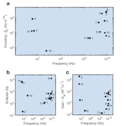
Figure 4: Analysis of experimental parameters for some representative experimental systems. (a), (b) and (c) show estimated continuum-optomechanical coupling constant, effective mechanical Q factor, and Brillouin gain. The horizontal axis displays the phonon frequency in each case. 1: Photonic crystal fibre (Kang et al 2009 kang_tightly_2009 ); 2,3: “Nanoweb” fibre (2 Butsch et al. 2012 butsch_optomechanical_2012 , 3 Butsch et al. 2014 butsch_cw-pumped_2014 ); 4: Chalcogenide ridge waveguide (Pant 2010 pant_-chip_2010 ); 5,7: Membrane suspended silicon waveguide (5 Shin et al. 2013 shin_tailorable_2013 , 7 Kittlaus et al. 2016 kittlaus_large_2016 ); 6,8: Silicon photonic nanowire (6 Laer et al. 2015 van_laer_interaction_2015 , 8 Laer et al. 2015 laer_net_2015 ); 9: Single-mode fibre (Behunin et al. 2015 behunin_long-lived_2015 ); 10: Helium filled hollow-core photonic crystal fiber (Renninger et al. 2016 renninger_nonlinear_2016 ); 11: Photonic crystal fibre (Kang et al. 2010 kang_all-optical_2010 ) 12: Silica nanowire fibre (Beugnot et al. 2014 beugnot_brillouin_2014 ); 13 Chalcogenide fibre (Abedin 2014 abedin_observation_2005 .); 14 “Nanoweb” fibre (Koehler et al. al. 2012 koehler_resolving_2016 )

Coupling between continuous optical and phonon fields has been realized in the context of nonlinear optics studies of Brillouin interactions. These experimental systems, depicted in Fig. 3, include step-index and micro-structured optical fibers abedin_observation_2005 ; beugnot_brillouin_2014 ; kang_tightly_2009 ; kang_all-optical_2010 ; butsch_optomechanical_2012 ; behunin_long-lived_2015 ; beugnot_guided_2007 , gas- and superfluid-filled photonic bandgap fiberszhong_depolarized_2015 ; renninger_guided-wave_2016 ; renninger_nonlinear_2016 ; renninger_forward_2016-1 , as well as chip-scale integrated optomechanical waveguide systems pant_-chip_2010 ; shin_tailorable_2013 ; shin_control_2015 ; van_laer_interaction_2015 ; laer_net_2015 ; kittlaus_large_2016 . To date, these studies have overwhelmingly focused on the Brillouin related nonlinear optical phenomena abedin_observation_2005 ; beugnot_brillouin_2014 ; kang_tightly_2009 ; kang_all-optical_2010 ; butsch_optomechanical_2012 ; behunin_long-lived_2015 ; beugnot_guided_2007 ; renninger_guided-wave_2016 ; renninger_nonlinear_2016 ; renninger_forward_2016-1 ; pant_-chip_2010 ; shin_tailorable_2013 ; shin_control_2015 ; van_laer_interaction_2015 ; laer_net_2015 ; kittlaus_large_2016 , as well as noise processes shelby_guided_1985 ; zhong_depolarized_2015 ; elser_reduction_2006 . However, it is also interesting to examine these systems through the lens of continuum optomechanics. Figure 4a shows the estimated continuum-optomechanical coupling strengths, extracted using the Brillouin gain $G_{B}$, as derived in the previous section. We see that couplings of between $10^{2}-10^{4}\leavevmode\nobreak\ \textup{Hz}\cdot\textup{m}^{1/2}$ have been realized using radiation pressure and (or) photo-elastic coupling. These couplings are mediated by phonons with frequencies between 10 MHz and 18 GHz depending on the type of interaction (intra-band or inter-band) and the elastic wave that mediates the coupling.

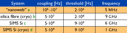
Figure 5: Possible experimental access to the strong coupling regime: The coupling $\left|\tilde{g}_{12}\right|$ needs to be much larger than the ’threshold’ $\sqrt{v_{2}/v_{b}}\Gamma/4$. Estimated values for a: koehler_resolving_2016 , b: behunin_long-lived_2015 , c: stimulated intermodal scattering in silicon (room temp.), d: same at $1K$, assuming an increase of $Q$ by a factor of 100.

The strength of the nonlinear optical susceptibility increases linearly with phononic Q-factor. This is seen by comparing the effective phononic Q-factors, plotted in Fig. 4b with the peak Brillouin gain of Fig. 4c. We define the effective Q-factor as the ratio of the mechanical frequency and the line-width. The effective Q-factor is always smaller than the intrinsic phonon Q-factor due to inhomogeneous broadening from variations in waveguide dimension along the waveguide length wolff_brillouin_2016 .

A variety of single-band (intra-modal) and multi-band (inter-modal) interactions have been demonstrated. These single-band processes include intra-modal forward-SBS processes (also termed stimulated Raman-like scattering) and backward-SBS processes; each process is denoted with circular and square markers, respectively, in Fig. 4. Multi-band processes, generically termed inter-modal Brillouin processes, are denoted by triangular markers in Fig. 4; their classification and nomenclature is discussed in the Suppl. Material.

As discussed in the previous section, the phonon coherence length has a significant impact on the spatio-temporal dynamics. Thus it is important to note that, depending on the intrinsic Q-factor and the type of phonon mode, the coherence length of the phonon can vary dramatically. For instance, since intra-modal coupling is mediated by phonons with vanishing group velocities ($\sim 1m/s$) shin_tailorable_2013 , phonon coherence lengths are often less than 100 nm. Conversely, in the cases of backward- or inter-modal (inter-band) coupling, the phonon group velocities can approach the intrinsic sound velocity in the waveguide material (e.g., $10^{4}m/s$). These higher velocity phonon modes correspond to 10-50 micron coherence lengths at room temperatures, but can be extended to milimeter length-scales at cryogenic temperaturesbehunin_long-lived_2015 .

Numerous nano-optomechanical devices have been proposed that have the potential to yield increased coupling strengths qiu_stimulated_2012 ; van_laer_analysis_2014 ; sarabalis_guided_2016 . Fig. 5 indicates the prospects for exploring the strong coupling regime discussed before.

XII Conclusions

We have established a connection between the continuum limit of optomechanical arrays and Brillouin physics. Especially studies of (classical and quantum) nonlinear dynamics will profit from our approach, where we categorized the simplest coupling terms and derived the quantum Langevin equations, including the noise terms and the correct boundary conditions. Applications such as wavelength conversion, phonon-induced coherent photon interactions and extensions to two-dimensional situations ruiz-rivas_dissipative_2016 ; butsch_optomechanical_2012-1 can now be analyzed on the basis of this framework. As an example, we have identified the strong coupling regime in continuum-optomechanical systems and prospects for reaching it in the context of state-of-the-art experimental systems.

Acknowledgements

We thank Philip Russell and Andrey Sukhorukov for initial discussions that helped inspire this project and for useful feedback on the manuscript. We acknowledge support by an ERC Starting Grant (FM). P.T.R. acknowledges support from the Packard Fellowship for Science and Engineering.

XIII Supplementary Material

XIII.1 Linearized Interaction

We briefly review the (straightforward) route from the fully nonlinear interaction to the linearized version, i.e. a quadratic Hamiltonian. Assume a steady state solution has been found, with $\beta(x)=\left\langle\hat{b}(x)\right\rangle$ and $\alpha(x)=\left\langle\hat{a}(x)\right\rangle$. As is known for standard cavity optomechanics, there might be more than one steady-state solution, and formally there could be an infinity of solutions for the continuum case. We have not explored this possibility further.

The deviations from this solution will now be denoted $\delta\hat{b}=\hat{b}-\beta$ and $\delta\hat{a}=\hat{a}-\alpha$. These are still fields. In contrast to the standard single-mode case, we will keep the possibility that $\beta(x)$ depends on position.

On the Hamiltonian level, we now obtain a new ’linearized’ (i.e. quadratic) interaction term:

$$-\hbar\int dx\,\left[\tilde{g}(x)\delta\hat{a}^{\dagger}(x)+\tilde{g}^{*}(x)\delta\hat{a}(x)\right]\left[\delta\hat{b}(x)+\delta\hat{b}^{\dagger}(x)\right]$$ (37)

as well as a term

$$-\hbar\int dx\,\tilde{g}_{\beta}(x)\delta\hat{a}^{\dagger}(x)\delta\hat{a}(x)\,,$$ (38)

which is a (possibly position-dependent) shift of the optical frequency. Its counterpart in the cavity optomechanics case is often dropped by an effective redefinition of the laser detuning.

In writing down Eq. (37), we have defined

$$\tilde{g}(x) \equiv \tilde{g}_{0}\alpha(x)$$ (39)

$$\tilde{g}_{\beta}(x) \equiv \tilde{g}_{0}(\beta(x)+\beta^{*}(x))$$ (40)

The photon-enhanced continuum coupling strength $\tilde{g}(x)$ is the direct analogue of the enhanced coupling $g=g_{0}\alpha$ in the standard linearized cavity-optomechanical case. In contrast to $\tilde{g}_{0}$, $\tilde{g}$ has the dimensions of a frequency. Likewise, $\tilde{g}_{\beta}$ is the static mechanical displacement, expressed as a resulting optical frequency shift.

At this point, we have only started from the simplest kind of interaction, Eq. (2), to obtain Eq. (37). We will comment on the other terms of table 1 below.

XIII.2 Optomechanical Arrays: Derivative Terms in the continuum version of the interaction

In an optomechanical array, it is possible to have an interaction that creates phononic excitations during the photon tunneling process: $-\hbar g_{0}(\hat{a}_{j+1}^{\dagger}\hat{a}_{j}+{\rm h.c.})\hat{u}_{j}$, where $\hat{u}_{j}\equiv\hat{b}_{j}+\hat{b}_{j}^{\dagger}$ describes the phonon displacement of a mode attached to the link between the sites $j$ and $j+1$. Here we describe how this can give rise to the canonical derivative terms when switching to a continuum description.

Switching from the discrete lattice model to the continuum model, we replace

$$\hat{a}_{j+1}^{\dagger}\hat{a}_{j}\hat{u}_{j}\mapsto\delta x^{3/2}\hat{a}^{\dagger}(x+\delta x/2)\hat{a}(x-\delta x/2)\hat{u}(x)\,,$$ (41)

where we chose coordinates so as to indicate that the phonon mode $\hat{u}$ is located halfway between the photon modes at $x\pm\delta x/2$. A Taylor expansion of

$$\hat{a}^{\dagger}(x+\delta x/2)\hat{a}(x-\delta x/2)+{\rm h.c.}$$ (42)

yields

$$2\hat{a}^{\dagger}\hat{a}+\left(\frac{\delta x}{2}\right)^{2}\left\{\left(\partial_{x}^{2}\hat{a}^{\dagger}\right)\hat{a}+\hat{a}^{\dagger}\left(\partial_{x}^{2}\hat{a}\right)-2\left(\partial_{x}\hat{a}^{\dagger}\right)\left(\partial_{x}\hat{a}\right)\right\}\,,$$ (43)

where all fields are taken at position $x$. Two things are worth noting here: First, all the first-order derivatives have disappeared (they would have violated inversion symmetry!). Second, we have obtained second-order derivatives of the photon field. If we want to turn this into our “canonical” choice of coupling terms (table 1), we have to integrate by parts, in which case derivatives may also act on $\hat{u}(x)$. This turns $\left\{\left(\partial_{x}^{2}\hat{a}^{\dagger}\right)\hat{a}+\hat{a}^{\dagger}\left(\partial_{x}^{2}\hat{a}\right)\right\}\hat{u}$ into:

$$-2(\partial_{x}\hat{a}^{\dagger})(\partial_{x}\hat{a})\hat{u}-\left[\left(\partial_{x}\hat{a}^{\dagger}\right)\hat{a}+\hat{a}^{\dagger}\left(\partial_{x}\hat{a}\right)\right]\left(\partial_{x}\hat{u}\right)\,.$$ (44)

Combining this with the other terms resulting from Eq. (43), one arrives at the interaction expressed completely in the canonical way.

XIII.3 Nonlinear susceptibility

We briefly discuss how, starting from the linearized Eq. (27), we can obtain the effective third-order nonlinear photon susceptibility induced by the interaction with the phonons. We slightly generalize this equation, by adding a possible detuning between the mechanical frequency $\Omega$ and the transition frequency $\Omega_{o}$ between the two optical branches:

$$\partial_{x}\left\langle\delta\hat{b}\right\rangle=i[(\Omega-\Omega_{o})/v_{b}]\left\langle\delta\hat{b}\right\rangle+i(\tilde{g}_{12}/v_{b})\left\langle\delta\hat{a}_{2}^{\dagger}\right\rangle-(\gamma_{b}/2)\left\langle\delta\hat{b}\right\rangle.$$ (45)

Solving for the steady state $\partial_{x}\left\langle\delta\hat{b}\right\rangle$ and inserting into the photon equation of motion, Eq. (26), we obtain:

$$\partial_{x}\left\langle\delta\hat{a}_{2}\right\rangle=-{\color[rgb]{1,0,0}{\normalcolor\frac{i}{v_{2}}}}\frac{\left|\tilde{g}_{0}(1,2)\right|^{2}\left|\alpha_{1}\right|^{2}{\color[rgb]{1,0,0}{\normalcolor\left\langle\delta\hat{a}_{2}\right\rangle}}}{\Omega-\Omega_{0}-i\frac{\Gamma}{2}}-\frac{\gamma_{2}}{2}\left\langle\delta\hat{a}_{2}\right\rangle\,.$$ (46)

We can express this as

$$\partial_{x}\left\langle\delta\hat{a}_{2}\right\rangle=i\gamma_{{\rm nonlin}}^{(3)}\left|\alpha_{1}\right|^{2}{\color[rgb]{1,0,0}{\normalcolor\left\langle\delta\hat{a}_{2}\right\rangle}}-\frac{\gamma_{2}}{2}\left\langle\delta\hat{a}_{2}\right\rangle\,,$$ (47)

with the effective nonlinear susceptibility

$$\gamma_{{\rm nonlin}}^{(3)}{\color[rgb]{1,0,0}{\normalcolor(\Omega)}}=-{\color[rgb]{1,0,0}{\normalcolor\frac{1}{v_{2}}}}\frac{\left|\tilde{g}_{0}(1,2)\right|^{2}}{\Omega-\Omega_{0}-i\frac{\Gamma}{2}}\,.$$ (48)

Using $P_{1}=\hbar\omega_{1}v_{1}\left|\alpha_{1}\right|^{2}$ and $P_{2}\cong\hbar\omega_{2}v_{2}\left|\left\langle\delta\hat{a}_{2}\right\rangle\right|^{2}$ to cast Eq. 47 in the form of Eq. 28, one finds that the frequency dependent gain is related to the nonlinear susceptibility as $G_{{\rm B}}(\Omega)=-2\cdot{\rm Im}\{\gamma_{{\rm nonlin}}^{(3)}(\Omega)\}(\hbar\omega_{1}v_{1})^{-1}$.

XIII.4 Types of Brillouin interactions

Here, we elucidate some naming conventions used in the Brillouin literature, and we explain how these names relate to the classifications that we use in this paper. These include (i) forward intra-band scattering processes, where incident and scattered light-fields co-propagate in the same optical mode, (ii) backward intra-band scattering processes, where the incident and scattered light-fields counter-propagate, as well as (iii) inter-band scattering processes, which generically describe processes that involve coupling between guided optical modes with distinct dispersion curves. Note that within Fig. 4 processes (i), (ii), and (iii) are identified by circular, square, and triangular markers, respectively.

Backward intra-band scattering processes, which is the most widely studied of Brillouin interactions, is commonly termed backward stimulated Brillouin scattering boyd_nonlinear_2013 ; agrawal_nonlinear_2012 ; references abedin_observation_2005 ; beugnot_brillouin_2014 ; behunin_long-lived_2015 ; beugnot_guided_2007 ; pant_-chip_2010 are examples of this process. However, for historical reasons, the terminology for forward intra-band and forward inter-band scattering processes is somewhat more diverse. Thermally driven (or spontaneous) forward intra-band scattering was first observed in optical fibers, and identified as a noise process, under the name guided acoustic wave Brillouin scattering (GAWBS) shelby_guided_1985 ; references zhong_depolarized_2015 ; elser_reduction_2006 are examples of this spontaneous process. Stimulated forward intra-band scattering processes have been described using the term (intra-modal) forward stimulated Brillouin scattering renninger_guided-wave_2016 ; renninger_nonlinear_2016 ; renninger_forward_2016-1 ; shin_tailorable_2013 ; shin_control_2015 ; van_laer_interaction_2015 ; laer_net_2015 ; kittlaus_large_2016 , as well as using the more descriptive term stimulated Raman-like scattering (SRLS) kang_all-optical_2010 ; butsch_optomechanical_2012 .

Inter-band processes have also been observed through both spontaneous and stimulated interactions under different names. Stimulated inter-band coupling between co-propagating guided optical modes with different polarization states has been termed stimulated inter-polarization scattering (SIPS) kang_all-optical_2010 . In the context of noise processes, the spontaneous version process has also been described using the term de-polarized GAWBS or depolarization scattering zhong_depolarized_2015 ; elser_reduction_2006 . Stimulated scattering between co-propagating guided optical modes with distinct spatial distribution has also been described using the term stimulated inter-modal scattering (SIMS) koehler_resolving_2016 and stimulated inter-modal Brillouin scattering qiu_stimulated_2013 .

References

- (1) Aspelmeyer, M., Kippenberg, T. J. & Marquardt, F. Cavity optomechanics. Reviews of Modern Physics 86, 1391–1452 (2014). URL http://link.aps.org/doi/10.1103/RevModPhys.86.1391.
- (2) Rakich, P. T., Reinke, C., Camacho, R., Davids, P. & Wang, Z. Giant Enhancement of Stimulated Brillouin Scattering in the Subwavelength Limit. Physical Review X 2, 011008 (2012). URL http://link.aps.org/doi/10.1103/PhysRevX.2.011008.
- (3) Van Laer, R., Kuyken, B., Van Thourhout, D. & Baets, R. Interaction between light and highly confined hypersound in a silicon photonic nanowire. Nature Photonics 9, 199–203 (2015). URL http://www.nature.com/nphoton/journal/v9/n3/abs/nphoton.2015.11.html.
- (4) Butsch, A., Koehler, J. R., Noskov, R. E. & Russell, P. S. CW-pumped single-pass frequency comb generation by resonant optomechanical nonlinearity in dual-nanoweb fiber. Optica 1, 158 (2014). URL https://www.osapublishing.org/optica/abstract.cfm?uri=optica-1-3-158.
- (5) Li, M. et al. Harnessing optical forces in integrated photonic circuits. Nature 456, 480–484 (2008). URL http://www.nature.com/nature/journal/v456/n7221/full/nature07545.html.
- (6) Bahl, G., Tomes, M., Marquardt, F. & Carmon, T. Observation of spontaneous Brillouin cooling. Nature Physics 8, 203–207 (2012). URL http://www.nature.com/nphys/journal/v8/n3/abs/nphys2206.html.
- (7) Bahl, G. et al. Brillouin cavity optomechanics with microfluidic devices. Nature Communications 4 (2013). URL http://www.nature.com/doifinder/10.1038/ncomms2994.
- (8) Shen, Y. R. & Bloembergen, N. Theory of Stimulated Brillouin and Raman Scattering. Physical Review 137, A1787–A1805 (1965). URL http://link.aps.org/doi/10.1103/PhysRev.137.A1787.
- (9) Shelby, R. M., Levenson, M. D. & Bayer, P. W. Guided acoustic-wave Brillouin scattering. Physical Review B 31, 5244–5252 (1985). URL http://link.aps.org/doi/10.1103/PhysRevB.31.5244.
- (10) Boyd, R. W. Nonlinear Optics (Academic Press, 2013). Google-Books-ID: _YpGBQAAQBAJ.
- (11) Agrawal, G. Nonlinear Fiber Optics (Academic Press, 2012). Google-Books-ID: SQOLP6M0socC.
- (12) Van Laer, R., Baets, R. & Van Thourhout, D. Unifying Brillouin scattering and cavity optomechanics. Physical Review A 93, 053828 (2016). URL http://link.aps.org/doi/10.1103/PhysRevA.93.053828.
- (13) Laude, V. & Beugnot, J.-C. Lagrangian description of Brillouin scattering and electrostriction in nanoscale optical waveguides. New Journal of Physics 17, 125003 (2015). URL http://stacks.iop.org/1367-2630/17/i=12/a=125003.
- (14) Sipe, J. E. & Steel, M. J. A Hamiltonian treatment of stimulated Brillouin scattering in nanoscale integrated waveguides. New Journal of Physics 18, 045004 (2016). URL http://stacks.iop.org/1367-2630/18/i=4/a=045004.
- (15) Zoubi, H. & Hammerer, K. Optomechanical Multi-Mode Hamiltonian for Nanophotonic Waveguides. arXiv:1604.07081 [physics, physics:quant-ph] (2016). URL http://arxiv.org/abs/1604.07081. ArXiv: 1604.07081.
- (16) Kharel, P., Behunin, R. O., Renninger, W. H. & Rakich, P. T. Noise and dynamics in forward Brillouin interactions. Physical Review A 93, 063806 (2016). URL http://link.aps.org/doi/10.1103/PhysRevA.93.063806.
- (17) Safavi-Naeini, A. H. et al. Two-Dimensional Phononic-Photonic Band Gap Optomechanical Crystal Cavity. Physical Review Letters 112, 153603 (2014). URL http://link.aps.org/doi/10.1103/PhysRevLett.112.153603.
- (18) Zhang, M., Shah, S., Cardenas, J. & Lipson, M. Synchronization and Phase Noise Reduction in Micromechanical Oscillator Arrays Coupled through Light. Physical Review Letters 115, 163902 (2015). URL http://link.aps.org/doi/10.1103/PhysRevLett.115.163902.
- (19) Chang, D., Safavi-Naeini, A. H., Hafezi, M. & Painter, O. Slowing and stopping light using an optomechanical crystal array. New Journal of Physics 13, 023003 (2011). URL http://arxiv.org/abs/1006.3829. ArXiv: 1006.3829.
- (20) Chen, W. & Clerk, A. A. Photon propagation in a one-dimensional optomechanical lattice. Physical Review A 89, 033854 (2014). URL http://link.aps.org/doi/10.1103/PhysRevA.89.033854.
- (21) Schmidt, M., Peano, V. & Marquardt, F. Optomechanical Dirac physics. New Journal of Physics 17, 023025 (2015). URL http://stacks.iop.org/1367-2630/17/i=2/a=023025.
- (22) Heinrich, G., Ludwig, M., Qian, J., Kubala, B. & Marquardt, F. Collective Dynamics in Optomechanical Arrays. Physical Review Letters 107, 043603 (2011). URL http://link.aps.org/doi/10.1103/PhysRevLett.107.043603.
- (23) Xuereb, A., Genes, C. & Dantan, A. Strong Coupling and Long-Range Collective Interactions in Optomechanical Arrays. Physical Review Letters 109, 223601 (2012). URL http://link.aps.org/doi/10.1103/PhysRevLett.109.223601.
- (24) Schmidt, M., Ludwig, M. & Marquardt, F. Optomechanical circuits for nanomechanical continuous variable quantum state processing. New Journal of Physics 14, 125005 (2012). URL http://stacks.iop.org/1367-2630/14/i=12/a=125005.
- (25) Xuereb, A., Genes, C., Pupillo, G., Paternostro, M. & Dantan, A. Reconfigurable Long-Range Phonon Dynamics in Optomechanical Arrays. Physical Review Letters 112, 133604 (2014). URL http://link.aps.org/doi/10.1103/PhysRevLett.112.133604.
- (26) Ludwig, M. & Marquardt, F. Quantum Many-Body Dynamics in Optomechanical Arrays. Physical Review Letters 111, 073603 (2013). URL http://link.aps.org/doi/10.1103/PhysRevLett.111.073603.
- (27) Schmidt, M., Kessler, S., Peano, V., Painter, O. & Marquardt, F. Optomechanical creation of magnetic fields for photons on a lattice. Optica 2, 635 (2015). URL https://www.osapublishing.org/abstract.cfm?URI=optica-2-7-635.
- (28) Peano, V., Brendel, C., Schmidt, M. & Marquardt, F. Topological Phases of Sound and Light. Physical Review X 5, 031011 (2015). URL http://link.aps.org/doi/10.1103/PhysRevX.5.031011.
- (29) Walter, S. & Marquardt, F. Dynamical Gauge Fields in Optomechanics. arXiv:1510.06754 [cond-mat, physics:quant-ph] (2015). URL http://arxiv.org/abs/1510.06754. ArXiv: 1510.06754.
- (30) Sarabalis, C. J., Hill, J. T. & Safavi-Naeini, A. H. Guided acoustic and optical waves in silicon-on-insulator for Brillouin scattering and optomechanics. APL Photonics 1, 071301 (2016). URL http://scitation.aip.org/content/aip/journal/app/1/7/10.1063/1.4955002;jsessionid=rWEuSqoS5AfOV2ePnqRK5USi.x-aip-live-03.
- (31) Wolff, C., Stiller, B., Eggleton, B. J., Steel, M. J. & Poulton, C. G. Cascaded forward Brillouin scattering to all Stokes orders. arXiv:1607.04740 [physics] (2016). URL http://arxiv.org/abs/1607.04740. ArXiv: 1607.04740.
- (32) Kang, M. S., Nazarkin, A., Brenn, A. & Russell, P. S. J. Tightly trapped acoustic phonons in photonic crystal fibres as highly nonlinear artificial Raman oscillators. Nature Physics 5, 276–280 (2009). URL http://www.nature.com/doifinder/10.1038/nphys1217.
- (33) Koehler, J. R. et al. Resolving the mystery of milliwatt-threshold opto-mechanical self-oscillation in dual-nanoweb fiber. APL Photonics 1, 056101 (2016). URL http://scitation.aip.org/content/aip/journal/app/1/5/10.1063/1.4953373.
- (34) Chiao, R. Y., Townes, C. H. & Stoicheff, B. P. Stimulated Brillouin Scattering and Coherent Generation of Intense Hypersonic Waves. Physical Review Letters 12, 592–595 (1964). URL http://link.aps.org/doi/10.1103/PhysRevLett.12.592.
- (35) Qiu, W. et al. Stimulated Brillouin scattering in nanoscale silicon step-index waveguides: a general framework of selection rules and calculating SBS gain. Optics express 21, 31402–31419 (2013). URL https://www.osapublishing.org/abstract.cfm?uri=oe-21-25-31402.
- (36) Wolff, C., Steel, M. J., Eggleton, B. J. & Poulton, C. G. Stimulated Brillouin scattering in integrated photonic waveguides: Forces, scattering mechanisms, and coupled-mode analysis. Physical Review A 92, 013836 (2015). URL http://link.aps.org/doi/10.1103/PhysRevA.92.013836.
- (37) Qiu, W., Rakich, P. T., Soljacic, M. & Wang, Z. Stimulated brillouin scattering in slow light waveguides. arXiv:1210.0738 [cond-mat, physics:physics] (2012). URL http://arxiv.org/abs/1210.0738. ArXiv: 1210.0738.
- (38) Zhu, Z., Gauthier, D. J. & Boyd, R. W. Stored Light in an Optical Fiber via Stimulated Brillouin Scattering. Science 318, 1748–1750 (2007). URL http://science.sciencemag.org/content/318/5857/1748.
- (39) Butsch, A. et al. Optomechanical Nonlinearity in Dual-Nanoweb Structure Suspended Inside Capillary Fiber. Physical Review Letters 109 (2012). URL http://link.aps.org/doi/10.1103/PhysRevLett.109.183904.
- (40) Abedin, K. S. Observation of strong stimulated Brillouin scattering in single-mode As 2 Se 3 chalcogenide fiber. Optics Express 13, 10266–10271 (2005). URL https://www.osapublishing.org/abstract.cfm?uri=oe-13-25-10266.
- (41) Behunin, R. O. et al. Long-lived guided phonons in fiber by manipulating two-level systems. arXiv preprint arXiv:1501.04248 (2015). URL http://arxiv.org/abs/1501.04248.
- (42) Pant, R. On-chip stimulated Brillouin scattering. Optics express 18, 19286–19291 (2010). URL https://www.osapublishing.org/abstract.cfm?uri=oe-18-18-19286.
- (43) Beugnot, J.-C., Sylvestre, T., Maillotte, H., Mélin, G. & Laude, V. Guided acoustic wave Brillouin scattering in photonic crystal fibers. Optics letters 32, 17–19 (2007). URL https://www.osapublishing.org/abstract.cfm?uri=ol-32-1-17.
- (44) Zhong, W. E. n. et al. Depolarized guided acoustic wave Brillouin scattering in hollow-core photonic crystal fibers. Optics Express 23, 27707 (2015). URL https://www.osapublishing.org/abstract.cfm?URI=oe-23-21-27707.
- (45) Renninger, W. H., Behunin, R. O. & Rakich, P. T. Guided-wave Brillouin scattering in air. arXiv:1607.04664 [physics] (2016). URL http://arxiv.org/abs/1607.04664. ArXiv: 1607.04664.
- (46) Renninger, W. H., Behunin, R. & Rakich, P. Nonlinear Optics in Superfluid Helium-Filled Hollow-Core Fiber. In CLEO: QELS Fundamental Science, FM4A–6 (Optical Society of America, 2016). URL https://www.osapublishing.org/abstract.cfm?uri=CLEO_QELS-2016-FM4A.6.
- (47) Renninger, W. H. et al. Forward Brillouin scattering in hollow-core photonic bandgap fibers. New Journal of Physics 18, 025008 (2016). URL http://stacks.iop.org/1367-2630/18/i=2/a=025008?key=crossref.88b1f3689f82412d83f886f230cf3cc7.
- (48) Laer, R. V., Bazin, A., Kuyken, B., Baets, R. & Thourhout, D. V. Net on-chip Brillouin gain based on suspended silicon nanowires. New Journal of Physics 17, 115005 (2015). URL http://stacks.iop.org/1367-2630/17/i=11/a=115005.
- (49) Beugnot, J.-C. et al. Brillouin light scattering from surface acoustic waves in a subwavelength-diameter optical fibre. Nature Communications 5, 5242 (2014). URL http://www.nature.com/ncomms/2014/141024/ncomms6242/full/ncomms6242.html?WT.ec_id=NCOMMS-20141029.
- (50) Shin, H. et al. Control of coherent information via on-chip photonic-phononic emitter-receivers. Nature Communications 6, 6427 (2015). URL http://www.nature.com/ncomms/2015/150305/ncomms7427/full/ncomms7427.html.
- (51) Shin, H. et al. Tailorable stimulated Brillouin scattering in nanoscale silicon waveguides. Nature Communications 4, 1944 (2013). URL http://www.nature.com/ncomms/2013/130606/ncomms2943/full/ncomms2943.html.
- (52) Kittlaus, E. A., Shin, H. & Rakich, P. T. Large Brillouin amplification in silicon. Nature Photonics 10, 463–467 (2016). URL http://www.nature.com/nphoton/journal/v10/n7/full/nphoton.2016.112.html.
- (53) Kang, M. S., Brenn, A. & St.J. Russell, P. All-Optical Control of Gigahertz Acoustic Resonances by Forward Stimulated Interpolarization Scattering in a Photonic Crystal Fiber. Physical Review Letters 105, 153901 (2010). URL http://link.aps.org/doi/10.1103/PhysRevLett.105.153901.
- (54) Elser, D. et al. Reduction of Guided Acoustic Wave Brillouin Scattering in Photonic Crystal Fibers. Physical Review Letters 97, 133901 (2006). URL http://link.aps.org/doi/10.1103/PhysRevLett.97.133901.
- (55) Wolff, C., Laer, R. V., Steel, M. J., Eggleton, B. J. & Poulton, C. G. Brillouin resonance broadening due to structural variations in nanoscale waveguides. New Journal of Physics 18, 025006 (2016). URL http://stacks.iop.org/1367-2630/18/i=2/a=025006.
- (56) Van Laer, R., Kuyken, B., Van Thourhout, D. & Baets, R. Analysis of enhanced stimulated Brillouin scattering in silicon slot waveguides. Optics Letters 39, 1242–1245 (2014). URL https://www.osapublishing.org/abstract.cfm?uri=ol-39-5-1242.
- (57) Ruiz-Rivas, J., Navarrete-Benlloch, C., Patera, G., Roldán, E. & de Valcárcel, G. J. Dissipative structures in optomechanical cavities. Physical Review A 93, 033850 (2016). URL http://link.aps.org/doi/10.1103/PhysRevA.93.033850.
- (58) Butsch, A., Conti, C., Biancalana, F. & Russell, P. S. Optomechanical Self-Channeling of Light in a Suspended Planar Dual-Nanoweb Waveguide. Physical Review Letters 108, 093903 (2012). URL http://link.aps.org/doi/10.1103/PhysRevLett.108.093903.