Ab initio dynamical vertex approximation

Abstract

Diagrammatic extensions of dynamical mean field theory (DMFT) such as the dynamical vertex approximation (D$\Gamma$A) allow us to include non-local correlations beyond DMFT on all length scales and proved their worth for model calculations. Here, we develop and implement an AbinitioD$\Gamma$A approach for electronic structure calculations of materials. Starting point is the two-particle irreducible vertex in the two particle-hole channels which is approximated by the bare non-local Coulomb interaction and all local vertex corrections. From this we calculate the full non-local vertex and the non-local self-energy through the Bethe-Salpeter equation. The AbinitioD$\Gamma$A approach naturally generates all local DMFT correlations and all non-local $GW$ contributions, but also further non-local correlations beyond: mixed terms of the former two and non-local spin fluctuations. We apply this new methodology to the prototypical correlated metal SrVO₃.

I Introduction

Some of the most fascinating physical phenomena are experimentally observed in strongly correlated electron systems and, on the theoretical side, only poorly understood hitherto. This is particularly true for electronic structure calculations of materials where the standard approach, density functional theory (DFT) Hohenberg and Kohn (1964); Kohn and Sham (1965); Jones and Gunnarsson (1989); Martin et al. (2004) in its local density approximation (LDA) or generalized gradient approximation (GGA) only rudimentarily includes such correlations. This calls for genuine many body techniques Martin (2016).

One such method is Hedin’s $GW$ approach Hedin (1965) consisting of the interacting Green’s function times the screened interaction $W$, which physically describes a screened exchange, see Fig. 1 top panel. In the last years, this approach has matured to the point that material calculations are actually feasible and various program packages are available. As a consequence, semiconductors, in which the extended $sp^{3}$ orbitals make the non-local exchange contribution particularly important, can be better described, especially their band gaps. From the point of view of the exchange-correlation potential of DFT, the $GW$ approach mostly improves upon the LDA or GGA regarding the exchange part. Via the inclusion of screening, $GW$ implicitly also includes correlation effects, leading to renormalized quasi-particle weights and finite life times. Nonetheless, in the presence of strong electronic correlations, e.g. in transition metal oxides and $f$-electron systems, the first order expression $GW$ of many-body perturbation theory is largely insufficient and vertex corrections become relevant.

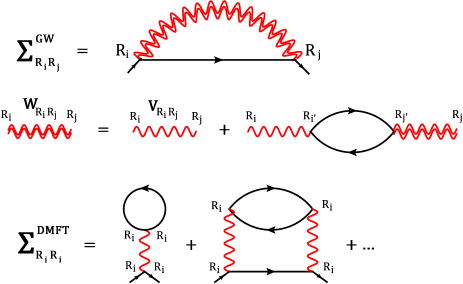
Figure 1: (Color online) Top: In addition to the Hartree term, $GW$ takes into account the (screened) exchange Feynman diagram (wiggled line: Coulomb interaction $V$; double wiggled line: screened interaction $W$; line: interacting Green’s function $G$; $\mathbf{R}_{i}$, $\mathbf{R}_{j}$ indicate the lattice sites). Middle: Calculation of $W$ as a screened Coulomb interaction within the RPA. Bottom: Feynman diagrams for the DMFT self-energy $\Sigma$.

For such strongly correlated materials, dynamical mean field theory (DMFT) Metzner and Vollhardt (1989); Georges and Kotliar (1992); Georges et al. (1996a) emerged instead as the state-of-the-art. The reason for this is that DMFT accounts for a major part of the electronic correlations, namely the local correlations between electrons on the same lattice site. These are particularly strong for transition metal oxides or heavy fermion systems with $d$- and $f$-electrons, respectively, due to the localized nature of the corresponding orbitals. Its merger with LDA Anisimov et al. (1997); Lichtenstein and Katsnelson (1998); Kotliar et al. (2006); Held (2007) or $GW$ Biermann et al. (2003); Tomczak et al. (2012a); Taranto et al. (2013); Sakuma et al. (2013); Tomczak et al. (2014); Tomczak (2015); Choi et al. (2016); Boehnke2016 ; Roekeghem2014 allows for realistic materials calculations and is more and more widely used. Does the principal method development of electronic structure calculations come to a standstill at this point? Or does it merely advance towards ever more complex and bigger systems?

In this paper, we show that a further big step forward is possible. Let us, to this end, start by analyzing $GW$ and DMFT, which are both based on Feynman diagrams: $GW$ simply takes (besides the Hartree term) the exchange diagram (Fig. 1 top) and much of its strengths result from the fact that this exchange term is taken in terms of the screened Coulomb interaction within the random phase approximation (RPA; Fig. 1 middle). This screening results in a much better convergence of the perturbation series of which actually only the first order terms are taken into account. DMFT, on the other hand, includes all local (skeleton) diagrams for the self-energy in terms of the interacting local Green’s function and Hubbard/Hund-like local interactions (Fig. 1 bottom). While this reliably accounts for the local electronic correlations, non-local correlations are neglected in DMFT. The same holds for extended DMFT Si and Smith (1996a); Chitra and Kotliar (2000) which treats the local correlations emerging from non-local interactions. The non-local correlations are, however, at the heart of some of the most fascinating phenomena associated with electronic correlations such as (quantum) criticality, spin fluctuations and, possibly, high-temperature superconductivity.

In this paper, we develop, implement and apply a 21${}^{\hbox{\tiny st}}$ century method for the ab initio calculation of correlated materials. It is based on recent diagrammatic extensions of DMFT Kusunose (2006); Toschi et al. (2007); Katanin et al. (2009); Rubtsov et al. (2008); Slezak et al. (2009); Rohringer et al. (2013); Taranto et al. (2014); Kitatani et al. (2015); Ayral and Parcollet (2015); Li (2015); Valli et al. (2015); Li et al. (2016), a development which started with the dynamical vertex approximation (D$\Gamma$A) Toschi et al. (2007); Katanin et al. (2009). These dynamical vertex approaches are quite similar and all based on the two-particle vertex instead of the one-particle vertex (i.e. the self-energy) in DMFT. This way, local dynamical correlations à la DMFT are captured but at the same time strong electronic correlations on all time and length scales are also included. In the context of many-body models, D$\Gamma$A and related approaches have been applied successfully to calculate, among others, (quantum) critical exponents,Rohringer et al. (2011); Antipov et al. (2014); Hirschmeier et al. (2015); Schäfer et al. (2016) and evidenced strong non-local contributions to the self-energy beyond GW.Schäfer et al. (2015)

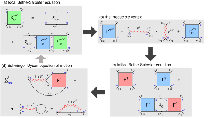
Figure 2: (Color online) Outline of the main equations of the AbinitioD$\Gamma$A approach: (a) The local Bethe-Salpeter equation allows extracting the local irreducible vertex $\Gamma_{loc}$ from the local generalized susceptibility $\chi_{loc}$. (b) The local irreducible vertex (which contains the local interaction $U$) is supplemented by the non-local interaction $V$ resulting in the momentum-dependent irreducible vertex $\Gamma$. (c) From this $\Gamma$ the full vertex $F$ is obtained using the Bethe-Salpeter equation (shown is only the particle-hole channel, but the related contribution from the transversal particle-hole channel is also included). (d) Finally, the self-energy is constructed via the Schwinger-Dyson equation consisting of the vertex part (top), and the Hartree-Fock contribution (bottom). From this self-energy one can, in principle, determine an updated local vertex, closing the loop. For details and the index convention, see Sec. II.3 and Sec. II.4.

One can also consider the first principles extension AbinitioD$\Gamma$A as a realization of Hedin’s idea Hedin (1965) to include vertex corrections beyond the $GW$ approximation. All vertex corrections which can be traced back to the irreducible local vertex in the particle-hole channels and the bare non-local Coulomb interaction are included, see Fig. 2(b). This seamlessly generates all the $GW$ diagrams and the associated physics, as well as the local diagrams of DMFT and non-local correlations beyond both on all length scales. Through the latter, we can describe, among others, phenomena such as quantum criticality, spin-fluctuation mediated superconductivity, and weak localization corrections to the conductivity. This is beyond DMFT which is restricted to local correlations as well as beyond $GW$ which is restricted to one screening channel and the low-coupling regime.Notevertexcorr Nonetheless, the computational effort of AbinitioD$\Gamma$A is still manageable even for materials calculations with several relevant orbitals, as we demonstrate in this work.

In Section II, we introduce the AbinitioD$\Gamma$A method, including all relevant equations. Section III, presents first results for the testbed material SrVO₃; and Section IV summarizes the work and provides an outlook for future applications. An avenue to AbinitioD$\Gamma$A was envisioned in Ref. Toschi et al., 2011. Here we concretize these ideas and fully derive and implement the approach. Please also note the proposal of Ref. Katanin, 2016 to use the functional renormalization group on top of the (extended) DMFT, and the dual boson approach Rubtsov et al. (2012) to non-local interactions.

II AbinitioD$\Gamma$A method

Before we go into the detailed multi-orbital derivation of the AbinitioD$\Gamma$A equations, let us briefly outline the rationale of the method, as it is depicted in Fig. 2.

As a starting point we consider a general Hamiltonian written in terms of a one-particle operator ($\widehat{H}_{0}$), and a two-particle interaction with a local ($\widehat{U}$) as well as a non-local ($\widehat{V}^{\mathbf{q}}$) part:

$$\widehat{H}=\widehat{H}_{0}+\widehat{U}+\sum_{{\mathbf{q}}}\widehat{V}^{{\mathbf{q}}}.$$ (1)

For AbinitioD$\Gamma$A calculations this Hamiltonian may contain a large set of orbitals, e.g., the physical $spdf$ orbitals in a muffin tin orbital basis set Andersen and Saha-Dasgupta (2000) or those obtained by a Wannier function projection Kuneš et al. (2010); Mostofi et al. (2008). However, the approach can also be applied to a more restricted set of orbitals for the low energy degrees of freedom such as the $t_{2g}$ orbitals for our SrVO₃ calculation in Section III. In the latter case, the influence of orbitals outside the energy windows of $\widehat{H}_{0}$ and their effect on $\widehat{H}_{0}$ have to be taken into account, e.g., on the DFT or $GW$ level. The screening of the interactions $\widehat{U}$ and $\widehat{V}^{{\mathbf{q}}}$ needs to be included as well, e.g., through constrained DFT Dederichs84 ; McMahan88 ; Gunnarsson89 or constrained RPA Aryasetiawan et al. (2004); Miyake and Aryasetiawan (2008); Tomczak et al. (2010).

AbinitioD$\Gamma$A is a Feynman diagrammatic theory built around the two-particle irreducible vertex which is approximated by the bare Coulomb interaction plus all local vertex corrections, see Fig. 2(b). From this irreducible vertex many additional Feynman diagrams are constructed. One has to distinguish between (i) the fully irreducible vertex as a starting point where these additional diagrams are constructed by the parquet equations as in Refs. Valli et al., 2015; Li et al., 2016 and (ii) the irreducible vertex in the particle-hole channel (and transversal particle hole channel) where this is done by the Bethe-Salpeter equations (BSE) as in Ref. Toschi et al., 2007; Katanin et al., 2009. For our realistic multi-orbital calculations we here rely on (ii) which is numerically more feasible.

To include the important local vertex corrections, first the local irreducible vertex $\Gamma_{loc}$ is extracted from the local two-particle Green’s function or from generalized susceptibilities $\chi_{loc}$ (see Fig. 2(a)). This is possible by solving an Anderson impurity model; and for multi-orbitals, continuous-time quantum Monte Carlo simulations Gull et al. (2011a); Boehnke14 ; Gunacker et al. (2015); Gunacker16 are most appropriate to this end. The resulting local irreducible vertices in the longitudinal and transversal particle-hole channels are then combined with the non-local interaction $V^{q}$ and finally dressed via the BSE equation (see Fig. 2(c); Sec. II.3). Eventually, a new lattice Green’s function is constructed using the $\mathbf{k}$-dependent self-energy calculated from the equation of motion (see Fig.  2(d); Sec. II.4).

In principle from the local projection of this new Green’s function an updated local vertex can be calculated as indicated by the arrow from Fig.  2 (d) to Fig.  2 (a). Such a self-consistent scheme has been envisaged in Refs. Held et al., 2008; Held, 2014; Ayral and Parcollet, 2016 but not yet implemented; it is of particular importance if the electron density changes considerably in D$\Gamma$A because the vertex and its asympotics depend strongly on the density. Beyond this, also the DFT Hamiltonian or the constrained RPA interaction and $GW$ self-energy for the high energy degrees of freedom should be updated through a charge Savrasov04 ; Minar05 ; Pouroskii07 ; Aichhorn2011 ; Bhandary16 or hermitianized self-energy P7:Faleev04 ; P7:Chantis06 self-consistency, respectively. These steps go beyond the one-shot calculation of the present paper where the local vertex is fixed to the DFT+DMFT solution.

As the computationally most demanding part is the calculation of the local vertex, it is reasonable (in case of a large set of orbitals) to calculate it only for the more correlated (e.g., $d$ and $f$) orbitals, whereas the local vertex of the less correlated (e.g., $spd$) orbitals may be taken as $U+V$ in the same way as the two $V$ terms in Fig. 2 (b). This includes all the GW diagrams for these orbitals but also Feynman diagrams beyond. NotebeyondGW A frequency dependence of $U(\omega)$ when using the constrained RPA as a starting point can also be included for the more correlated orbitals in the same way, i.e., adding $U(\omega)-U$ to the vertex.noteHirayama Alternatively, one can calculate the local vertex from $U(\omega)$ in CT-QMC.

Let us after these general considerations, now turn to the actual equations and technical details of the AbinitioD$\Gamma$A approach. Fig. 2 provides an overview, but the devil is in the details and Fig. 2 is somewhat schematic: We have not specified the spin-indices and have only shown the longitudinal (not the transversal) particle-hole channel; also, in our implementation, we circumvent an explicit evaluation of $\Gamma_{loc}$ as this quantity may contain divergencies; we also show how to increase the numerical efficiency by a reformulation in terms of three-leg quantities and by neglecting—as an additional approximation—the ${\mathbf{k}},{\mathbf{k}}^{\prime}$ dependence of the irreducible vertex in Fig. 2 (b).

II.1 Coulomb interaction

The electron-electron Coulomb interaction $\widehat{U}^{{\mathrm{full}}}$ can in general be expressed as

$$\widehat{U}^{{\mathrm{full}}} = \frac{1}{2}\sum_{\begin{subarray}{c}\mathbf{R}_{1},\mathbf{R}_{2},\mathbf{R}_{3}\\ ll^{\prime}mm^{\prime}\\ \sigma\sigma^{\prime}\end{subarray}}U^{{\mathrm{full}}}_{lm^{\prime}ml^{\prime}}(\mathbf{R}_{1},\mathbf{R}_{2},\mathbf{R}_{3})\times$$

$$\times \widehat{c}^{\dagger}_{{\mathbf{R}_{3}m^{\prime}\sigma}}\widehat{c}^{\dagger}_{\mathbf{R}_{1}l\sigma^{\prime}}\widehat{c}^{\phantom{\dagger}}_{\mathbf{R}_{2}m\sigma^{\prime}}\widehat{c}^{\phantom{\dagger}}_{\mathbf{0}l^{\prime}\sigma},$$

where the Roman indices $ll^{\prime}mm^{\prime}$ denote the orbitals, $\sigma$ the spin, and $\mathbf{R}$ the lattice site. It fulfills the particle “swapping symmetry”

$$U^{{\mathrm{full}}}_{lm^{\prime}ml^{\prime}}(\mathbf{R}_{1},\mathbf{R}_{2},\mathbf{R}_{3})=U^{{\mathrm{full}}}_{m^{\prime}ll^{\prime}m}(\mathbf{R}_{3}-\mathbf{R}_{2},-\mathbf{R}_{2},\mathbf{R}_{1}-\mathbf{R}_{2}),$$ (3)

which corresponds to an invariance under a swap of both the incoming and the outgoing particle labels. Taking the Fourier transform with respect to $\mathbf{R}$ yields

$$U^{{\mathbf{q}}{\mathbf{k}}{\mathbf{k}}^{\prime}}_{lm^{\prime}ml^{\prime}} =\sum_{\mathbf{R}_{1},\mathbf{R}_{2},\mathbf{R}_{3}}e^{i{\mathbf{k}}\mathbf{R}_{1}}e^{-i({\mathbf{k}}-{\mathbf{q}})\mathbf{R}_{2}}e^{i({\mathbf{k}}^{\prime}-{\mathbf{q}})\mathbf{R}_{3}}$$

$$\times U^{{\mathrm{full}}}_{lm^{\prime}ml^{\prime}}(\mathbf{R}_{1},\mathbf{R}_{2},\mathbf{R}_{3})\;;$$ (4)

or for the interaction operator

$$\widehat{U}^{{\mathrm{full}}}=\frac{1}{2}\sum_{\begin{subarray}{c}{\mathbf{q}}{\mathbf{k}}{\mathbf{k}}^{\prime}\\ ll^{\prime}mm^{\prime}\\ \sigma\sigma^{\prime}\end{subarray}}U^{{\mathbf{q}}{\mathbf{k}}{\mathbf{k}}^{\prime}}_{lm^{\prime}ml^{\prime}}\widehat{c}^{\dagger}_{{\mathbf{k}}^{\prime}-{\mathbf{q}}m^{\prime}\sigma}\widehat{c}^{\dagger}_{{\mathbf{k}}l\sigma^{\prime}}\widehat{c}^{\phantom{\dagger}}_{{\mathbf{k}}-{\mathbf{q}}m\sigma^{\prime}}\widehat{c}^{\phantom{\dagger}}_{{\mathbf{k}}^{\prime}l^{\prime}\sigma},$$ (5)

where

$$\widehat{c}_{{\mathbf{k}}l\sigma} =\sum_{\mathbf{R}}e^{i{\mathbf{k}}\mathbf{R}}\widehat{c}_{\mathbf{R}l\sigma}.$$ (6)

The k-point dependence of $\widehat{U}^{{\mathrm{full}}}$ can be simplified if the orbital overlap between adjacent unit-cells is neglected, so that the creation and annihilation operators are paired up at site $\mathbf{0}$ and $\mathbf{R}$. This gives

$$U_{lm^{\prime}ml^{\prime}} \equiv U^{{\mathrm{full}}}_{lm^{\prime}ml^{\prime}}(\mathbf{0},\mathbf{0},\mathbf{0}),$$ (7)

$$V^{{\mathbf{q}}}_{lm^{\prime}ml^{\prime}} \equiv\sum_{\mathbf{R}\neq 0}e^{i\mathbf{R}{\mathbf{q}}}U^{{\mathrm{full}}}_{lm^{\prime}ml^{\prime}}(\mathbf{R},\mathbf{R},\mathbf{0}),$$ (8)

which corresponds to a local interaction $\widehat{U}$ and a purely non-local interaction $\widehat{V}^{\mathbf{q}}$. In this case the swapping symmetry reduces to $U_{lm^{\prime}ml^{\prime}}=U_{m^{\prime}ll^{\prime}m}$ and $V^{{\mathbf{q}}}_{lm^{\prime}ml^{\prime}}=V^{-{\mathbf{q}}}_{m^{\prime}ll^{\prime}m}$.

II.2 Green’s functions

We begin with the basic definitions of the one- and two-particle Green’s functions

$$G^{{\mathbf{k}}}_{\sigma,lm}(\tau) \equiv-\left\langle\!{\mathcal{T}}\!\left[\widehat{c}^{\phantom{\dagger}}_{\mathbf{k}l\sigma}(\tau)\widehat{c}^{\dagger}_{\mathbf{k}m\sigma}(0)\right]\!\right\rangle,$$ (9)

$$G^{{\mathbf{q}}{\mathbf{k}}{\mathbf{k}}^{\prime}}_{\begin{subarray}{c}lmm^{\prime}l^{\prime}\\ \sigma_{1}\sigma_{2}\sigma_{3}\sigma_{4}\end{subarray}}(\tau_{1},\tau_{2},\tau_{3}) \equiv$$ (10)

$$\left\langle\!{\mathcal{T}}\!\left[\widehat{c}^{\phantom{\dagger}}_{\mathbf{k}l\sigma_{1}}(\tau_{1})\widehat{c}^{\dagger}_{{\mathbf{k}}-{\mathbf{q}}m\sigma_{2}}(\tau_{2})\widehat{c}^{\phantom{\dagger}}_{{\mathbf{k}}^{\prime}-{\mathbf{q}}m^{\prime}\sigma_{3}}(\tau_{3})\widehat{c}^{\dagger}_{\mathbf{k}^{\prime}l^{\prime}\sigma_{4}}(0)\right]\!\right\rangle.$$

where $\tau\in[0,\beta)$ denotes imaginary time and ${\mathcal{T}}$ is the time ordering operator. In absence of spin-orbit interaction the spin is conserved, which leaves 6 different spin combinations

$$G^{{\mathbf{q}}{\mathbf{k}}{\mathbf{k}}^{\prime}}_{\sigma\sigma^{\prime},lmm^{\prime}l^{\prime}}(\tau_{1},\tau_{2},\tau_{3}) \equiv G^{{\mathbf{q}}{\mathbf{k}}{\mathbf{k}}^{\prime}}_{\begin{subarray}{c}lmm^{\prime}l^{\prime}\\ \sigma\sigma\sigma^{\prime}\sigma^{\prime}\end{subarray}}(\tau_{1},\tau_{2},\tau_{3}),$$ (11)

$$G^{{\mathbf{q}}{\mathbf{k}}{\mathbf{k}}^{\prime}}_{\overline{\sigma\sigma^{\prime}},lmm^{\prime}l^{\prime}}(\tau_{1},\tau_{2},\tau_{3}) \equiv G^{{\mathbf{q}}{\mathbf{k}}{\mathbf{k}}^{\prime}}_{\begin{subarray}{c}lmm^{\prime}l^{\prime}\\ \sigma\sigma^{\prime}\sigma^{\prime}\sigma\end{subarray}}(\tau_{1},\tau_{2},\tau_{3}).$$ (12)

There are only two independent spin configurations in the paramagnetic phase, as the system then is SU(2) symmetric with respect to the spin,

$$G_{\sigma\sigma^{\prime}} =G_{(-\sigma)(-\sigma^{\prime})}=G_{\sigma^{\prime}\sigma},$$ (13)

$$G_{\sigma\sigma} =G_{\sigma(-\sigma)}+G_{\overline{\sigma(-\sigma)}}.$$ (14)

As we will see in the next section, one particularly useful choice for these two spin combinations is the density and magnetic channel defined as

$$G_{d} =G_{\uparrow\uparrow}+G_{\uparrow\downarrow},$$ (15)

$$G_{m} =G_{\uparrow\uparrow}-G_{\uparrow\downarrow}=G_{\overline{\uparrow\downarrow}}.$$ (16)

The value of the two-particle Green’s function takes a step of 1 whenever the $\tau$ arguments of a creation and an annihilation operator become equal. These discontinuities can be cancelled out by subtracting pairs of one-particle Green’s functions, giving the so-called connected part of the two-particle Green’s function

$$G^{{\mathrm{con~{}}}{\mathbf{q}}{\mathbf{k}}{\mathbf{k}}^{\prime}}_{\sigma\sigma^{\prime},lmm^{\prime}l^{\prime}}(\tau_{1},\tau_{2},\tau_{3})=G^{{\mathbf{q}}{\mathbf{k}}{\mathbf{k}}^{\prime}}_{\sigma\sigma^{\prime},lmm^{\prime}l^{\prime}}(\tau_{1},\tau_{2},\tau_{3})$$

$$\quad\;\;\;-\,\delta_{{\mathbf{q}}0}G^{{\mathbf{k}}}_{\sigma,lm}(\tau_{1}-\tau_{2})G^{{\mathbf{k}}^{\prime}}_{\sigma^{\prime},m^{\prime}l^{\prime}}(\tau_{3})$$

$$\quad\;\;\;+\,\delta_{\sigma\sigma^{\prime}}\delta_{{\mathbf{k}}{\mathbf{k}}^{\prime}}G^{{\mathbf{k}}}_{\sigma,ll^{\prime}}(\tau_{1})G^{{\mathbf{k}}-{\mathbf{q}}}_{\sigma,m^{\prime}m}(\tau_{3}-\tau_{2}).$$ (17)

The connected part is continuous in its $\tau$ arguments, but it still shows cusps at equal times. We define the Fourier transformation of $G^{{\mathrm{con~{}}}}$ with respect to $\tau$ in the same way as for $\widehat{U}^{{\mathrm{full}}}$ and $\mathbf{R}$,

$$G^{{\mathrm{con~{}}}{\mathrm{q}}{\mathrm{k}}{\mathrm{k}}^{\prime}}_{\sigma\sigma^{\prime},lmm^{\prime}l^{\prime}} \!=\!\int_{0}^{\beta}\!\!\int_{0}^{\beta}\!\!\int_{0}^{\beta}\!\!d\tau_{1}d\tau_{2}d\tau_{3}e^{i\nu\tau_{1}}e^{-i(\nu-\omega)\tau_{2}}e^{i(\nu^{\prime}-\omega)\tau_{3}}$$

$$\times G^{{\mathrm{con~{}}}{\mathbf{q}}{\mathbf{k}}{\mathbf{k}}^{\prime}}_{\sigma\sigma^{\prime},lmm^{\prime}l^{\prime}}(\tau_{1},\tau_{2},\tau_{3}),$$ (18)

where the bosonic compound index is ${\mathrm{q}}=(\omega,{\mathbf{q}})$ and the fermionic compound index ${\mathrm{k}}=(\nu,{\mathbf{k}})$. In the chosen frequency and momentum convention the bosonic index (${\mathrm{q}}$) corresponds to a longitudinal transfer of energy and momentum from one particle-hole pair ($ml$) to the other ($m^{\prime}l^{\prime}$).

$G^{{\mathrm{con~{}}}}$ is by definition related to the fully reducible vertex $F$ as

$$G^{{\mathrm{con~{}}}{\mathrm{q}}{\mathrm{k}}{\mathrm{k}}^{\prime}}_{r,lmm^{\prime}l^{\prime}}=\sum_{nn^{\prime}hh^{\prime}}\chi^{{\mathrm{q}}{\mathrm{k}}{\mathrm{k}}}_{0,lmhn}F^{{\mathrm{q}}{\mathrm{k}}{\mathrm{k}}^{\prime}}_{r,nhh^{\prime}n^{\prime}}\chi^{{\mathrm{q}}{\mathrm{k}}^{\prime}{\mathrm{k}}^{\prime}}_{0,n^{\prime}h^{\prime}m^{\prime}l^{\prime}},$$ (19)

where the bare 2-particle propagator $\chi_{0}$ is defined as

$$\chi^{{\mathrm{q}}{\mathrm{k}}{\mathrm{k}}^{\prime}}_{0,lmm^{\prime}l^{\prime}}\equiv-\beta G^{{\mathrm{k}}}_{ll^{\prime}}G^{{\mathrm{k}}^{\prime}-{\mathrm{q}}}_{mm^{\prime}}\delta_{{\mathrm{k}}{\mathrm{k}}^{\prime}}.$$ (20)

The full vertex $F$ is part of the definition of the Bethe-Salpeter equation (BSE), and will thus be of major importance in the diagrammatic extension outlined in the next section.

In order to improve the statistics of the two-particle Green’s function, and reduce the computational resources needed to perform the calculations, it is important to utilize the symmetries of the system. In addition to the orbital symmetries the two-particle Green’s function also fulfills time reversal symmetry,

$$G^{{\mathrm{q}}{\mathrm{k}}{\mathrm{k}}^{\prime}}_{\sigma\sigma^{\prime},lmm^{\prime}l^{\prime}}=G^{\bar{{\mathrm{q}}}\bar{{\mathrm{k}}^{\prime}}\bar{{\mathrm{k}}}}_{\sigma^{\prime}\sigma,l^{\prime}m^{\prime}ml},$$ (21)

where $\bar{{\mathrm{k}}}=\{\nu,-{\mathbf{k}}\}$, and the crossing symmetries,

$$G^{{\mathrm{q}}{\mathrm{k}}{\mathrm{k}}^{\prime}}_{\sigma\sigma^{\prime},lmm^{\prime}l^{\prime}} =-G^{({\mathrm{k}}^{\prime}-{\mathrm{k}})({\mathrm{k}}^{\prime}-{\mathrm{q}}){\mathrm{k}}^{\prime}}_{\overline{\sigma^{\prime}\sigma},m^{\prime}mll^{\prime}}$$ (22)

$$=-G^{({\mathrm{k}}-{\mathrm{k}}^{\prime}){\mathrm{k}}({\mathrm{k}}-{\mathrm{q}})}_{\overline{\sigma\sigma^{\prime}},ll^{\prime}m^{\prime}m}$$ (23)

$$=G^{(-{\mathrm{q}})({\mathrm{k}}^{\prime}-{\mathrm{q}})({\mathrm{k}}-{\mathrm{q}})}_{\sigma^{\prime}\sigma,m^{\prime}l^{\prime}lm},$$ (24)

where the last line corresponds to a full swap of the in-coming and the outgoing particle labels. The symmetries Eqs. (22-24) can be understood from the fact that exchanging the position of the “legs” does not alter the vertex but the $q,k,k^{\prime}$ values it corresponds tp as visualized in Fig. 3. Finally, the two-particle Green’s function transforms under complex conjugation as

$$(G^{{\mathrm{q}}{\mathrm{k}}{\mathrm{k}}^{\prime}}_{\sigma\sigma^{\prime},lmm^{\prime}l^{\prime}})^{*}=G^{(-{\mathrm{q}})(-{\mathrm{k}})(-{\mathrm{k}}^{\prime})}_{\sigma^{\prime}\sigma,l^{\prime}m^{\prime}ml}.$$ (25)

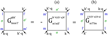
Figure 3: Diagrammatic representation of (a) the crossing symmetry in Eq. (22) and (b) the swapping symmetry in Eq. (24).

II.3 Diagrammatic extension

At the heart of the AbinitioD$\Gamma$A method is the two-particle irreducible vertex $\Gamma$ in the particle-hole channel

$$\Gamma^{{\mathrm{q}}{\mathrm{k}}{\mathrm{k}}^{\prime}}_{\sigma\sigma^{\prime},lmm^{\prime}l^{\prime}} \equiv\Gamma^{\omega\nu\nu^{\prime}}_{\sigma\sigma^{\prime},lmm^{\prime}l^{\prime}}+{\mathbf{V}}^{{\mathbf{q}}{\mathbf{k}}{\mathbf{k}}^{\prime}}_{\sigma\sigma^{\prime},lmm^{\prime}l^{\prime}},$$ (26)

$${\mathbf{V}}^{{\mathbf{q}}{\mathbf{k}}{\mathbf{k}}^{\prime}}_{\sigma\sigma^{\prime},lmm^{\prime}l^{\prime}} \equiv\beta^{-2}(V^{{\mathbf{q}}}_{lm^{\prime}ml^{\prime}}-\delta_{\sigma\sigma^{\prime}}V^{{\mathbf{k}}^{\prime}-{\mathbf{k}}}_{mm^{\prime}ll^{\prime}}),$$ (27)

given by the local irreducible vertex $\Gamma^{\omega\nu\nu^{\prime}}$ supplemented with the non-local interaction ${\mathbf{V}}^{{\mathbf{q}}{\mathbf{k}}{\mathbf{k}}^{\prime}}$ written in the form of a fully irreducible vertex, as shown in Fig. 2(b). For brevity we omit here and in the following in $\Gamma^{\omega\nu\nu^{\prime}}$ a “loc” subscript [which is implied if the vertex depends on frequencies only; please recall the convention ${\mathrm{q}}=(\omega,{\mathbf{q}})$ and ${\mathrm{k}}=(\nu,{\mathbf{k}})$] and a “ph” subscript ($\Gamma$’s and later $\phi$’s without an explicit subscript refer to the particle-hole channel). As already mentioned, $\Gamma$ can be extracted from the solution of an effective Anderson impurity problem through the inversion of a local BSE, which relates the local two-particle irreducible ($\Gamma$) and reducible ($\phi$) vertices in the particle-hole channel with the local full vertex

$$F^{\omega\nu\nu^{\prime}}_{r,lmm^{\prime}l^{\prime}} =\Gamma^{\omega\nu\nu^{\prime}}_{r,lmm^{\prime}l^{\prime}}+\phi^{\omega\nu\nu^{\prime}}_{r,lmm^{\prime}l^{\prime}},$$ (28)

$$\phi^{\omega\nu\nu^{\prime}}_{r,lmm^{\prime}l^{\prime}} =\sum_{\begin{subarray}{c}nn^{\prime}hh^{\prime}\\ \nu^{\prime\prime}\end{subarray}}\Gamma^{\omega\nu\nu^{\prime\prime}}_{r,lmhn}\chi^{\omega\nu^{\prime\prime}\nu^{\prime\prime}}_{0,nhh^{\prime}n^{\prime}}F^{\omega\nu^{\prime\prime}\nu^{\prime}}_{r,n^{\prime}h^{\prime}m^{\prime}l^{\prime}}.$$ (29)

Here $r\in\{d,m\}$ denotes the (d)ensity or the (m)agnetic spin combination as in Eqs. (15) and (16) which allows us to decouple the spin components. The local full vertex $F$ can in turn be obtained via Eq. (19) from the local 2-particle Green’s function $G^{{\mathrm{con~{}}}}$, which can be directly calculated in continuous-time quantum Monte Carlo. Equivalently, $\Gamma$ can also be directly obtained from the local BSE of local generalized susceptibilities,

$$\chi^{\omega\nu\nu^{\prime}}_{r,lmm^{\prime}l^{\prime}}=\chi^{\omega\nu\nu^{\prime}}_{0,lmm^{\prime}l^{\prime}}\delta_{\nu\nu^{\prime}}+\sum_{\begin{subarray}{c}nn^{\prime}hh^{\prime}\\ \nu^{\prime\prime}\end{subarray}}\chi^{\omega\nu\nu}_{0,lmhn}\Gamma^{\omega\nu\nu^{\prime\prime}}_{r,nhh^{\prime}n^{\prime}}\chi^{\omega\nu^{\prime\prime}\nu^{\prime}}_{r,n^{\prime}h^{\prime}m^{\prime}l^{\prime}},$$ (30)

as depicted in Fig. 2(a).

The BSE extends the “swapping” symmetry in Eq. (24) of $F$ to $\phi$ and $\Gamma$, but not the crossing symmetry in Eqs. (22) and (23), i.e.,

$$\phi^{\omega\nu\nu^{\prime}}_{r,lmm^{\prime}l^{\prime}} =\phi^{(-\omega)(\nu^{\prime}-\omega)(\nu-\omega)}_{r,m^{\prime}l^{\prime}lm},$$ (31)

$$\phi^{\omega\nu\nu^{\prime}}_{r,lmm^{\prime}l^{\prime}} \neq\phi^{\omega\nu\nu^{\prime}}_{\overline{ph},r,lmm^{\prime}l^{\prime}},$$ (32)

$$\phi^{\omega\nu\nu^{\prime}}_{\overline{ph},\sigma\sigma^{\prime},lmm^{\prime}l^{\prime}} =-\phi^{(\nu^{\prime}-\nu)(\nu^{\prime}-\omega)\nu^{\prime}}_{\overline{\sigma^{\prime}\sigma},m^{\prime}mll^{\prime}}$$ (33)

$$=-\phi^{(\nu-\nu^{\prime})\nu(\nu-\omega)}_{\overline{\sigma^{\prime}\sigma},ll^{\prime}m^{\prime}m},$$ (34)

where the transversal particle-hole channel ($\overline{ph}$) by definition is antisymmetric to the particle-hole channel with respect to a relabelling of the two incoming or outgoing particles. Applying the SU(2) symmetry relations in Eq. (14) to $\phi_{\overline{ph}}$ gives the explicit relations

$$\phi^{\omega\nu\nu^{\prime}}_{\overline{ph},d,lmm^{\prime}l^{\prime}} =-\frac{1}{2}\phi^{(\nu^{\prime}-\nu)(\nu^{\prime}-\omega)\nu^{\prime}}_{d,m^{\prime}mll^{\prime}}-\frac{3}{2}\phi^{(\nu^{\prime}-\nu)(\nu^{\prime}-\omega)\nu^{\prime}}_{m,m^{\prime}mll^{\prime}},$$ (35)

$$\phi^{\omega\nu\nu^{\prime}}_{\overline{ph},m,lmm^{\prime}l^{\prime}} =-\frac{1}{2}\phi^{(\nu^{\prime}-\nu)(\nu^{\prime}-\omega)\nu^{\prime}}_{d,m^{\prime}mll^{\prime}}+\frac{1}{2}\phi^{(\nu^{\prime}-\nu)(\nu^{\prime}-\omega)\nu^{\prime}}_{m,m^{\prime}mll^{\prime}},$$ (36)

or in the case of a non-local BSE

$$\phi^{{\mathrm{q}}{\mathrm{k}}{\mathrm{k}}^{\prime}}_{\overline{ph},d,lmm^{\prime}l^{\prime}} =-\frac{1}{2}\phi^{({\mathrm{k}}^{\prime}-{\mathrm{k}})({\mathrm{k}}^{\prime}-{\mathrm{q}}){\mathrm{k}}^{\prime}}_{d,m^{\prime}mll^{\prime}}-\frac{3}{2}\phi^{({\mathrm{k}}^{\prime}-{\mathrm{k}})({\mathrm{k}}^{\prime}-{\mathrm{q}}){\mathrm{k}}^{\prime}}_{m,m^{\prime}mll^{\prime}},$$ (37)

$$\phi^{{\mathrm{q}}{\mathrm{k}}{\mathrm{k}}^{\prime}}_{\overline{ph},m,lmm^{\prime}l^{\prime}} =-\frac{1}{2}\phi^{({\mathrm{k}}^{\prime}-{\mathrm{k}})({\mathrm{k}}^{\prime}-{\mathrm{q}}){\mathrm{k}}^{\prime}}_{d,m^{\prime}mll^{\prime}}+\frac{1}{2}\phi^{({\mathrm{k}}^{\prime}-{\mathrm{k}})({\mathrm{k}}^{\prime}-{\mathrm{q}}){\mathrm{k}}^{\prime}}_{m,m^{\prime}mll^{\prime}}.$$ (38)

From the starting point $\Gamma^{{\mathrm{q}}{\mathrm{k}}{\mathrm{k}}^{\prime}}_{r}$ in Eq. (26), we now need to construct the full vertex $F^{{\mathrm{q}}{\mathrm{k}}{\mathrm{k}}^{\prime}}_{r}$ through a non-local BSE. In the following we will focus on the longitudinal particle-hole channel, but the final expressions will also contain the BSE diagrams for the transversal particle-hole channel through the use of Eqs.(37) and (38). The third channel, the particle-particle channel, is considered here to be local in nature and already well described by its local contribution in $\Gamma^{\omega\nu\nu^{\prime}}$.

The non-local BSE in the particle-hole channel is given by

$$F^{{\mathrm{q}}{\mathrm{k}}{\mathrm{k}}^{\prime}}_{r,lmm^{\prime}l^{\prime}} =\Gamma^{{\mathrm{q}}{\mathrm{k}}{\mathrm{k}}^{\prime}}_{r,lmm^{\prime}l^{\prime}}+\sum_{\begin{subarray}{c}nn^{\prime}hh^{\prime}\\ {\mathrm{k}}^{\prime\prime}\end{subarray}}\Gamma^{{\mathrm{q}}{\mathrm{k}}{\mathrm{k}}^{\prime\prime}}_{r,lmhn}\chi^{{\mathrm{q}}{\mathrm{k}}^{\prime\prime}{\mathrm{k}}^{\prime\prime}}_{0,nhh^{\prime}n^{\prime}}F^{{\mathrm{q}}{\mathrm{k}}^{\prime\prime}{\mathrm{k}}^{\prime}}_{r,n^{\prime}h^{\prime}m^{\prime}l^{\prime}}.$$ (39)

A considerable simplification of this equation is possible if $\Gamma^{{\mathrm{q}}{\mathrm{k}}{\mathrm{k}}^{\prime}}$ does not depend on the momenta ${\mathbf{k}}$ and ${\mathbf{k}}^{\prime}$. Indeed this dependence arises only from the second (crossed) $V^{{\mathbf{k}}^{\prime}-{\mathbf{k}}}$ term in Eq. (27) which is neglected e.g. in the $GW$ approach. If we follow $GW$ and neglect this term or average it over ${\mathbf{k}}$ (which gives zero since $V$ was defined as purely non-local), the vertex (now already in the two spin channels $r\in\{d,m\}$) reads

$$\Gamma^{{\mathrm{q}}\nu\nu^{\prime}}_{r,lmm^{\prime}l^{\prime}}=\Gamma^{\omega\nu\nu^{\prime}}_{r,lmm^{\prime}l^{\prime}}+2\beta^{-2}V^{{\mathbf{q}}}_{lm^{\prime}ml^{\prime}}\delta_{r,d}.$$ (40)

and the BSE becomes (see Fig. 2(c))

$$F^{{\mathrm{q}}{\mathrm{k}}{\mathrm{k}}^{\prime}}_{r,lmm^{\prime}l^{\prime}}=\Gamma^{{\mathrm{q}}\nu\nu^{\prime}}_{r,lmm^{\prime}l^{\prime}}+\sum_{\begin{subarray}{c}nn^{\prime}hh^{\prime}\\ {\mathrm{k}}^{\prime\prime}\end{subarray}}\Gamma^{{\mathrm{q}}\nu\nu^{\prime\prime}}_{r,lmhn}\chi^{{\mathrm{q}}{\mathrm{k}}^{\prime\prime}{\mathrm{k}}^{\prime\prime}}_{0,nhh^{\prime}n^{\prime}}F^{{\mathrm{q}}{\mathrm{k}}^{\prime\prime}{\mathrm{k}}^{\prime}}_{r,n^{\prime}h^{\prime}m^{\prime}l^{\prime}}.$$ (41)

Since $\Gamma_{r}$ is now independent of ${\mathbf{k}}$ and ${\mathbf{k}}^{\prime}$, this will also be the case for $F$ in Eq. (41). The summation over ${\mathbf{k}}^{\prime\prime}$ hence yields

$$F^{{\mathrm{q}}\nu\nu^{\prime}}_{r,lmm^{\prime}l^{\prime}} =\Gamma^{{\mathrm{q}}\nu\nu^{\prime}}_{r,lmm^{\prime}l^{\prime}}+\phi^{{\mathrm{q}}\nu\nu^{\prime}}_{r,lmm^{\prime}l^{\prime}}$$ (42)

$$\phi^{{\mathrm{q}}\nu\nu^{\prime}}_{r,lmm^{\prime}l^{\prime}} =\sum_{\begin{subarray}{c}nn^{\prime}hh^{\prime}\\ \nu^{\prime\prime}\end{subarray}}\Gamma^{{\mathrm{q}}\nu\nu^{\prime\prime}}_{r,lmhn}\chi^{{\mathrm{q}}\nu^{\prime\prime}\nu^{\prime\prime}}_{0,nhh^{\prime}n^{\prime}}F^{{\mathrm{q}}\nu^{\prime\prime}\nu^{\prime}}_{r,n^{\prime}h^{\prime}m^{\prime}l^{\prime}},$$ (43)

$$\chi^{{\mathrm{q}}\nu\nu}_{0,lmm^{\prime}l^{\prime}} =\sum_{{\mathbf{k}}}\chi^{{\mathrm{q}}{\mathrm{k}}{\mathrm{k}}}_{0,lmm^{\prime}l^{\prime}}.$$ (44)

By combining the left (right) orbital indices and fermionic Matsubara frequencies into a single compound index $\{lm,\nu\}$ ($\{l^{\prime}m^{\prime},\nu^{\prime}\}$) Eq. (42) can be written as a matrix equation in terms of these compound indices:

$$F^{{\mathrm{q}}}_{r} =\Gamma^{{\mathrm{q}}}_{r}+\phi^{{\mathrm{q}}}_{r}=\Gamma^{{\mathrm{q}}}_{r}+\Gamma^{{\mathrm{q}}}_{r}\chi^{{\mathrm{q}}}_{0}F^{{\mathrm{q}}}_{r}.$$ (45)

The full vertex $F$ can now, in principle, be extracted from Eq. (45) through a simple matrix inversion

$$F^{{\mathrm{q}}}_{r}=\left[(\Gamma^{{\mathrm{q}}}_{r})^{-1}-\chi^{{\mathrm{q}}}_{0}\right]^{-1}.$$ (46)

However, as recently shown in Ref. Schaefer et al., 2016 the local $\Gamma$ extracted from a self-consistent DMFT calculation contains an infinite set of diverging components. The numerical complications associated with these diverging components can be avoided by substituting the local $\Gamma$ in Eq. (46) by the local $F$ using Eqs. (28) and (29). After some algebra this yields

$$F^{{\mathrm{q}}}_{d}= \Big{(}F^{\omega}_{d}+2\beta^{-2}V^{{\mathbf{q}}}({\mathbf{1}}+\chi^{\omega}_{0}F^{\omega}_{d})\Big{)}\times$$

$$\Big{[}{\mathbf{1}}-\chi^{nl,{\mathrm{q}}}_{0}F^{\omega}_{d}-2\beta^{-2}\chi^{{\mathrm{q}}}_{0}V^{{\mathbf{q}}}({\mathbf{1}}+\chi^{\omega}_{0}F^{\omega}_{d})\Big{]}^{-1}\!\!\!\!\!\!\!,$$ (47)

$$F^{{\mathrm{q}}}_{m}= F^{\omega}_{m}\Big{[}{\mathbf{1}}-\chi^{nl,{\mathrm{q}}}_{0}F^{\omega}_{m}\Big{]}^{-1}$$ (48)

where the purely non-local $\chi^{nl}$ is defined as

$$\chi^{nl,{\mathrm{q}}}_{0}\equiv\chi^{{\mathrm{q}}}_{0}-\chi^{\omega}_{0}.$$ (49)

This formulation is equivalent to Eq. (46) but circumvents the aforementioned divergencies in the local $\Gamma$.

The non-local full vertices generated in Eqs. (47) and (48) through only the particle-hole channel are not crossing symmetric [the vertices are not antisymmetric with respect to a relabelling of the two in-coming or outgoing particles, as in Eqs. (22) and (23)]. The crossing symmetry is however restored if we take the corresponding diagrams in the transversal particle-hole channel into account as well, as done before for a single orbital Toschi et al. (2007); Katanin et al. (2009). That is, in the parquet equation we add the reducible contributions in the particle-hole and transversal particle-hole channel and subtract their respective local contribution which is already contained in the local $F$:

$${\mathbf{F}}^{{\mathrm{q}}{\mathrm{k}}{\mathrm{k}}^{\prime}}_{d,lmm^{\prime}l^{\prime}}= F^{\omega\nu\nu^{\prime}}_{d,lmm^{\prime}l^{\prime}}+{\mathbf{V}}^{{\mathbf{q}}{\mathbf{k}}{\mathbf{k}}^{\prime}}_{d,lmm^{\prime}l^{\prime}}+(\phi^{{\mathrm{q}}\nu\nu^{\prime}}_{d,lmm^{\prime}l^{\prime}}-\phi^{\omega\nu\nu^{\prime}}_{d,lmm^{\prime}l^{\prime}})$$

$$+(\phi^{{\mathrm{q}}{\mathrm{k}}{\mathrm{k}}^{\prime}}_{\overline{ph},d,lmm^{\prime}l^{\prime}}-\phi^{\omega\nu\nu^{\prime}}_{\overline{ph},d,lmm^{\prime}l^{\prime}}).$$ (50)

Here, we consider the particle-particle channel and all fully irreducible diagrams, except ${\mathbf{V}}^{{\mathbf{q}}{\mathbf{k}}{\mathbf{k}}^{\prime}}$, to be local. The bare non-local interaction vertex ${\mathbf{V}}^{{\mathbf{q}}{\mathbf{k}}{\mathbf{k}}^{\prime}}$ defined in Eq. (27) has to be added explicitly to the parquet equation since it is neither part of the reducible vertices $\phi_{ph}$ and $\phi_{\overline{ph}}$, nor the local $F$.

Resolving Eqs. (28) and (42) for $\phi$, Eq. (40) for $\Gamma$, and taking the difference of the local and non-local $\phi$ yields

$$(\phi^{{\mathrm{q}}\nu\nu^{\prime}}_{d,lmm^{\prime}l^{\prime}}-\phi^{\omega\nu\nu^{\prime}}_{d,lmm^{\prime}l^{\prime}})= ~{}F^{nl,{\mathrm{q}}\nu\nu^{\prime}}_{d,lmm^{\prime}l^{\prime}}-2\beta^{-2}V^{{\mathbf{q}}}_{lm^{\prime}ml^{\prime}},$$ (51)

where the (full) non-local vertex $F^{nl}$ is defined as

$$F^{nl,{\mathrm{q}}\nu\nu^{\prime}}_{r,lmm^{\prime}l^{\prime}}\equiv F^{{\mathrm{q}}\nu\nu^{\prime}}_{r,lmm^{\prime}l^{\prime}}-F^{\omega\nu\nu^{\prime}}_{r,lmm^{\prime}l^{\prime}}.$$ (52)

For the transversal particle-hole channel we can calculate the same difference by subtracting Eq. (35) from Eq. (37) and expressing all terms by $F$ similar as in Eq. (51). This yields

$$(\phi^{{\mathrm{q}}{\mathrm{k}}{\mathrm{k}}^{\prime}}_{\overline{ph},d,lmm^{\prime}l^{\prime}}-\phi^{\omega\nu\nu^{\prime}}_{\overline{ph},d,lmm^{\prime}l^{\prime}})= -\frac{1}{2}F^{nl,({\mathrm{k}}^{\prime}-{\mathrm{k}})(\nu^{\prime}-\omega)\nu^{\prime}}_{d,m^{\prime}mll^{\prime}}$$

$$-\frac{3}{2}F^{nl,({\mathrm{k}}^{\prime}-{\mathrm{k}})(\nu^{\prime}-\omega)\nu^{\prime}}_{m,m^{\prime}mll^{\prime}}$$

$$+\beta^{-2}V^{{\mathbf{k}}^{\prime}-{\mathbf{k}}}_{m^{\prime}lml^{\prime}}.$$ (53)

Eqs. (51) and (53) can now be used in Eq. (50) to finally give

$${\mathbf{F}}^{{\mathrm{q}}{\mathrm{k}}{\mathrm{k}}^{\prime}}_{d,lmm^{\prime}l^{\prime}}= F^{\omega\nu\nu^{\prime}}_{d,lmm^{\prime}l^{\prime}}+F^{nl,{\mathrm{q}}\nu\nu^{\prime}}_{d,lmm^{\prime}l^{\prime}}-\frac{1}{2}F^{nl,({\mathrm{k}}^{\prime}-{\mathrm{k}})(\nu^{\prime}-\omega)\nu^{\prime}}_{d,m^{\prime}mll^{\prime}}$$

$$-\frac{3}{2}F^{nl,({\mathrm{k}}^{\prime}-{\mathrm{k}})(\nu^{\prime}-\omega)\nu^{\prime}}_{m,m^{\prime}mll^{\prime}},$$ (54)

where the non-local $F^{nl}$ is defined in Eq. (52) with $F^{{\mathrm{q}}}$ from the reformulated BSEs (47) or (48).

It should be noted that the two non-crossing symmetric contributions to the bare non-local interaction $V$ in Eq. (51) and (53) add up to become exactly $V^{{\mathbf{q}}{\mathbf{k}}{\mathbf{k}}^{\prime}}$ as defined in Eq. (27). This is unique to the simplification employed in Eq. (40).

II.4 Equation of motion

Besides the BSE, the equation of motion or Schwinger-Dyson equation is the second central equation of the AbinitioD$\Gamma$A approach. It allows us to calculate the self-energy from the crossing symmetric full vertex (or the connected two-particle Green’s function). For deriving the multi-orbital Schwinger-Dyson equation, we compare the $\tau$-derivative of $G^{{\mathbf{k}}}_{\sigma,lm}(\tau)$ in the Heisenberg equation of motion with the Dyson equation. This yields

$${\left[\Sigma G\right]^{{\mathbf{k}}}_{\sigma,mm^{\prime}}(\tau)=\left\langle\!{\mathcal{T}}\!\left[\left[\widehat{U}^{{\mathrm{full}}},\widehat{c}^{\phantom{\dagger}}_{{\mathbf{k}}m\sigma}(\tau)\right]\widehat{c}^{\dagger}_{\mathbf{k}m^{\prime}\sigma}(0)\right]\!\right\rangle}$$

$$=\sum_{\begin{subarray}{c}lhn\sigma^{\prime}\\ {\mathbf{q}}{\mathbf{k}}^{\prime}\end{subarray}}\left(U_{mlhn}+\mathbf{V}^{{\mathbf{q}}}_{mlhn}\right)\times$$

$$\times\left\langle\!{\mathcal{T}}\!\left[\widehat{c}^{\dagger}_{{\mathbf{k}}^{\prime}-{\mathbf{q}}l\sigma^{\prime}}(\tau)\widehat{c}^{\phantom{\dagger}}_{{\mathbf{k}}-{\mathbf{q}}h\sigma}(\tau)\widehat{c}^{\phantom{\dagger}}_{{\mathbf{k}}^{\prime}n\sigma^{\prime}}(\tau)\widehat{c}^{\dagger}_{{\mathbf{k}}m^{\prime}\sigma}(0)\right]\!\right\rangle$$

$$=\!\lim_{\tau^{\prime}\rightarrow\tau^{+}}\!\sum_{\begin{subarray}{c}lhn\sigma^{\prime}\\ {\mathbf{q}}{\mathbf{k}}^{\prime}\end{subarray}}\left(U_{mlhn}+\mathbf{V}^{{\mathbf{q}}}_{mlhn}\right)G^{{\mathbf{q}}{\mathbf{k}}^{\prime}{\mathbf{k}}}_{\sigma^{\prime}\sigma,nlhm^{\prime}}(\tau,\tau^{\prime},\tau)$$ (55)

where, in the second line, we have used the swapping symmetry for $U_{lm^{\prime}ml^{\prime}}$ and $\mathbf{V}^{{\mathbf{q}}}_{lm^{\prime}ml^{\prime}}$. The limit in Eq. (55) can be taken by splitting the two-particle Green’s function into its connected and disconnected parts using Eq. (17):

$${\left[\Sigma G\right]^{{\mathbf{k}}}_{\sigma,mm^{\prime}}(\tau)=\sum_{\begin{subarray}{c}lhn\sigma^{\prime}\\ {\mathbf{q}}{\mathbf{k}}^{\prime}\end{subarray}}\left(U_{mlhn}+\mathbf{V}^{{\mathbf{q}}}_{mlhn}\right)\times}$$

$$\times\left[G^{{\mathrm{con~{}}}{\mathbf{q}}{\mathbf{k}}^{\prime}{\mathbf{k}}}_{\sigma^{\prime}\sigma,nlhm^{\prime}}(\tau,\tau,\tau)+\delta_{{\mathbf{q}}0}n^{{\mathbf{k}}^{\prime}}_{\sigma^{\prime},ln}G^{{\mathbf{k}}}_{\sigma^{\prime},hm^{\prime}}(\tau)\right.$$

$$\;\;\;\;\left.-\delta_{\sigma\sigma^{\prime}}\delta_{{\mathbf{k}}{\mathbf{k}}^{\prime}}n^{{\mathbf{k}}-{\mathbf{q}}}_{\sigma,lh}G^{{\mathbf{k}}}_{\sigma,nm^{\prime}}(\tau)\right],$$ (56)

where $n_{mm^{\prime}}=\langle\widehat{c}^{\dagger}_{m}\widehat{c}^{\phantom{\dagger}}_{m^{\prime}}\rangle$. Taking the Fourier transform with respect to $\tau$ gives

$$\left[\Sigma G\right]^{{\mathrm{k}}}_{\sigma,mm^{\prime}}=\sum_{\begin{subarray}{c}lhh^{\prime}n\sigma^{\prime}\\ {\mathbf{q}}{\mathbf{k}}^{\prime}\end{subarray}}\left(U_{mlhn}+\mathbf{V}^{{\mathbf{q}}}_{mlhn}\right)$$

$$\times\left[\int_{0}^{\beta}e^{i\nu\tau}G^{{\mathrm{con~{}}}{\mathbf{q}}{\mathbf{k}}^{\prime}{\mathbf{k}}}_{\sigma^{\prime}\sigma,nlh^{\prime}m^{\prime}}(\tau,\tau,\tau)d\tau\right.$$

$$\;\;\;\;\left.+\delta_{{\mathbf{q}}0}n^{{\mathbf{k}}^{\prime}}_{\sigma^{\prime},ln}G^{{\mathrm{k}}}_{\sigma^{\prime},h^{\prime}m^{\prime}}-\delta_{\sigma\sigma^{\prime}}\delta_{{\mathbf{k}}{\mathbf{k}}^{\prime}}n^{{\mathbf{k}}-{\mathbf{q}}}_{\sigma,lh}G^{{\mathrm{k}}}_{\sigma,nm^{\prime}}\right].$$ (57)

Since the connected part is continuous it is possible to obtain the equal time component in Eq. (57) by simply summing up the bosonic and the left fermionic Matsubara frequencies

$$\int_{0}^{\beta}d\tau e^{i\nu\tau}G^{{\mathrm{con~{}}}{\mathbf{q}}{\mathbf{k}}^{\prime}{\mathbf{k}}}_{\sigma^{\prime}\sigma,nlh^{\prime}m^{\prime}}(\tau,\tau,\tau)=\frac{1}{\beta^{2}}\sum_{\omega\nu^{\prime}}G^{{\mathrm{con~{}}}{\mathrm{q}}{\mathrm{k}}^{\prime}{\mathrm{k}}}_{\sigma^{\prime}\sigma,nlh^{\prime}m^{\prime}}.$$ (58)

Finally, multiplying with $G^{-1}$ from the right yields the multi-orbital Schwinger-Dyson equation

$$\Sigma^{{\mathrm{k}}}_{\sigma,mm^{\prime}} =\Sigma^{{\mathrm{HF~{}}}{\mathbf{k}}}_{\sigma,mm^{\prime}}+\Sigma^{{\mathrm{con~{}}}{\mathrm{k}}}_{\sigma,mm^{\prime}},$$ (59)

$$\Sigma^{{\mathrm{con~{}}}{\mathrm{k}}}_{\sigma,mm^{\prime}} =\beta^{-2}\sum_{\begin{subarray}{c}ll^{\prime}hn\\ \sigma^{\prime}{\mathrm{q}}{\mathrm{k}}^{\prime}\end{subarray}}\!\Big{(}U_{mlhn}+\mathbf{V}^{{\mathbf{q}}}_{mlhn}\Big{)}G^{{\mathrm{con~{}}}{\mathrm{q}}{\mathrm{k}}^{\prime}{\mathrm{k}}}_{\sigma^{\prime}\sigma,nlhl^{\prime}}[G^{{\mathrm{k}}}_{\sigma}]^{-1}_{l^{\prime}m^{\prime}},$$ (60)

where $\Sigma^{{\mathrm{HF}}}$ is the static Hartree-Fock contribution to the self-energy.

Since we would like to calculate the self-energy starting from ${{F}}$ in Eq. (54), let us recall that we assume SU(2) symmetry and apply the relation between ${{F}}$ and $G^{{\mathrm{con}}}$ in Eq. (19). This yields the multi-orbital Schwinger-Dyson equation

$$\Sigma^{{\mathrm{con~{}}}{\mathrm{k}}}_{mm^{\prime}}=-\beta^{-1}\sum_{\begin{subarray}{c}ll^{\prime}nn^{\prime}hh^{\prime}\\ {\mathrm{q}}{\mathrm{k}}^{\prime}\end{subarray}}\! \Big{(}U_{mlhn}+\mathbf{V}^{{\mathbf{q}}}_{mlhn}\Big{)}\times$$ (61)

$$\times\chi^{{\mathrm{q}}{\mathrm{k}}^{\prime}{\mathrm{k}}^{\prime}}_{0,nll^{\prime}n^{\prime}}F^{{\mathrm{q}}{\mathrm{k}}^{\prime}{\mathrm{k}}}_{d,n^{\prime}l^{\prime}h^{\prime}m^{\prime}}G^{{\mathrm{k}}-{\mathrm{q}}}_{hh^{\prime}},$$

that finally determines the non-local AbinitioD$\Gamma$A self-energy.

In the following we present some implementational details. That is, we split Eq. (61) into contributions of the particle-hole and transversal particle-hole terms of Eq. (54) as well into the $U$ and $\mathbf{V}^{{\mathbf{q}}}$ terms. This yields, suppressing the orbital indices for clarity as they remain identical to those in Eq. (61):

$$\Sigma^{Uloc,{\mathrm{k}}}= -\beta^{-1}\sum_{{\mathrm{q}}\nu^{\prime}}\!U\chi^{{\mathrm{q}}\nu^{\prime}\nu^{\prime}}_{0}F^{\omega\nu^{\prime}\nu}_{d}G^{{\mathrm{k}}-{\mathrm{q}}},$$ (62)

$$\Sigma^{Vloc,{\mathrm{k}}}= -\beta^{-1}\sum_{{\mathrm{q}}\nu^{\prime}}\!\mathbf{V}^{{\mathbf{q}}}\chi^{{\mathrm{q}}\nu^{\prime}\nu^{\prime}}_{0}F^{\omega\nu^{\prime}\nu}_{d}G^{{\mathrm{k}}-{\mathrm{q}}},$$ (63)

$$\Sigma^{ph,{\mathrm{k}}}= -\beta^{-1}\sum_{{\mathrm{q}}\nu^{\prime}}\!\Big{(}U+\mathbf{V}^{{\mathbf{q}}}\Big{)}\chi^{{\mathrm{q}}\nu^{\prime}\nu^{\prime}}_{0}F^{nl,{\mathrm{q}}\nu^{\prime}\nu}_{d}G^{{\mathrm{k}}-{\mathrm{q}}},$$ (64)

$$\Sigma^{U\overline{ph},{\mathrm{k}}}= \beta^{-1}\sum_{{\mathrm{q}}\nu^{\prime}}\!\tilde{U}\chi^{{\mathrm{q}}\nu^{\prime}\nu^{\prime}}_{0}\times$$ (65)

$$\times\Big{(}\frac{1}{2}F^{nl,{\mathrm{q}}\nu^{\prime}\nu}_{d}+\frac{3}{2}F^{nl,{\mathrm{q}}\nu^{\prime}\nu}_{m}\Big{)}G^{{\mathrm{k}}-{\mathrm{q}}},$$

$$\Sigma^{V\overline{ph},{\mathrm{k}}}= \beta^{-1}\sum_{{\mathrm{q}}\nu^{\prime}}\!\tilde{V}^{{\mathbf{k}}^{\prime}-{\mathbf{k}}}\chi^{{\mathrm{q}}{\mathrm{k}}^{\prime}{\mathrm{k}}^{\prime}}_{0}\times$$ (66)

$$\times\Big{(}\frac{1}{2}F^{nl,{\mathrm{q}}\nu^{\prime}\nu}_{d}+\frac{3}{2}F^{nl,{\mathrm{q}}\nu^{\prime}\nu}_{m}\Big{)}G^{{\mathrm{k}}-{\mathrm{q}}},$$

where $\tilde{U}_{lm^{\prime}l^{\prime}m}=U_{lm^{\prime}ml^{\prime}}$ and similarly for $V$. The indices in the terms originating from the transversal particle-hole channel have been relabelled to make the full vertices $F$ depend on ${\mathbf{q}}$ instead of ${\mathbf{k}}^{\prime}-{\mathbf{k}}$. Indeed, the way Eq. (61) is written might suggest that the particle-hole and transversal particle-hole channels are treated differently. This is however not the case since an application of the crossing symmetry of $F$ together with the swapping symmetry of the interaction leaves Eq. (61) unchanged, but swaps the role of the particle-hole and transversal particle-hole channels in $F$. In the BSE ladders we have, in Eq. (40) and similar to $GW$, included $\mathbf{V}^{\mathbf{q}}$ but not $\mathbf{V}^{{\mathbf{k}}^{\prime}-{\mathbf{k}}}$. Against this background, it is reasonable to omit $\Sigma^{V\overline{ph}}$ for consistency.

In the following we will take advantage of the particular momentum and frequency structure of the Schwinger-Dyson equation to optimize the numerical calculation of the self-energy. To this end we define three three-legged quantities (cf. Refs. Katanin et al., 2009; Ayral and Parcollet, 2015) with increasing order of non-local character:

$$\gamma^{\omega\nu}_{r,lmm^{\prime}l^{\prime}} \equiv\sum_{n^{\prime}h^{\prime}\nu^{\prime}}\chi^{\omega\nu^{\prime}\nu^{\prime}}_{0,lmn^{\prime}h^{\prime}}F^{\omega\nu^{\prime}\nu}_{r,h^{\prime}n^{\prime}m^{\prime}l^{\prime}},$$ (67)

$$\gamma^{{\mathrm{q}}\nu}_{r,lmm^{\prime}l^{\prime}} \equiv\sum_{n^{\prime}h^{\prime}\nu^{\prime}}\chi^{nl,{\mathrm{q}}\nu^{\prime}\nu^{\prime}}_{0,lmn^{\prime}h^{\prime}}F^{\omega\nu^{\prime}\nu}_{r,h^{\prime}n^{\prime}m^{\prime}l^{\prime}},$$ (68)

$$\eta^{{\mathrm{q}}\nu}_{r,lmm^{\prime}l^{\prime}} \equiv\sum_{n^{\prime}h^{\prime}\nu^{\prime}}\chi^{{\mathrm{q}}\nu^{\prime}\nu^{\prime}}_{0,lmn^{\prime}h^{\prime}}F^{{\mathrm{q}}\nu^{\prime}\nu}_{r,h^{\prime}n^{\prime}m^{\prime}l^{\prime}}-\chi^{\omega\nu^{\prime}\nu^{\prime}}_{0,lmn^{\prime}h^{\prime}}F^{\omega\nu^{\prime}\nu}_{r,h^{\prime}n^{\prime}m^{\prime}l^{\prime}}.$$ (69)

Here, $\gamma^{\omega\nu}$ is strictly local and can be extracted directly from the impurity solverHafermann et al. (2012); Gunacker16 ; $\gamma^{{\mathrm{q}}\nu}$ contains the local full vertex connected to a purely non-local bare two-particle propagator. The vertex $\eta^{{\mathrm{q}}\nu}$ describes the full vertex connected to the bare two-particle propagator, but with all purely local diagrams removed. It can be calculated efficiently from Eqs. (47) and (48) using a matrix inversion and $\gamma^{\omega}_{r}$:

$$\eta^{{\mathrm{q}}}_{r} =(\vec{{\mathbf{1}}}+\gamma^{\omega}_{r})\times$$ (70)

$$\times\Big{(}\Big{[}{\mathbf{1}}-\chi^{nl,{\mathrm{q}}}_{0}F^{\omega}_{r}-2\beta^{-2}\chi^{{\mathrm{q}}}_{0}\mathbf{V}^{{\mathbf{q}}}(\vec{{\mathbf{1}}}+\gamma^{\omega}_{r})\delta_{rd}\Big{]}^{-1}-{\mathbf{1}}\Big{)},$$

where $\vec{{\mathbf{1}}}_{lmm^{\prime}l^{\prime}}=\delta_{ll^{\prime}}\delta_{mm^{\prime}}$. The self-energy can now be written in terms of $\gamma$ and $\eta$.

$$\Sigma^{Uloc,{\mathrm{k}}}= \Sigma^{\nu}_{{\mathrm{DMFT}}}-\beta^{-1}\sum_{{\mathrm{q}}}\!U\gamma^{{\mathrm{q}}}_{d}G^{{\mathrm{k}}-{\mathrm{q}}},$$ (71)

$$\Sigma^{Vloc,{\mathrm{k}}}= -\beta^{-1}\sum_{{\mathrm{q}}}\!\mathbf{V}^{{\mathbf{q}}}(\gamma^{{\mathrm{q}}}_{d}+\gamma^{\omega}_{d})G^{{\mathrm{k}}-{\mathrm{q}}},$$ (72)

$$\Sigma^{ph,{\mathrm{k}}}= -\beta^{-1}\sum_{{\mathrm{q}}}\!\Big{(}U+\mathbf{V}^{{\mathbf{q}}}\Big{)}(\eta^{{\mathrm{q}}}_{d}-\gamma^{{\mathrm{q}}}_{d})G^{{\mathrm{k}}-{\mathrm{q}}},$$ (73)

$$\Sigma^{U\overline{ph},{\mathrm{k}}}= \beta^{-1}\sum_{{\mathrm{q}}}\!\tilde{U}\Big{[}\frac{1}{2}(\eta^{{\mathrm{q}}}_{d}-\gamma^{{\mathrm{q}}}_{d})+\frac{3}{2}(\eta^{{\mathrm{q}}}_{m}-\gamma^{{\mathrm{q}}}_{m})\Big{]}G^{{\mathrm{k}}-{\mathrm{q}}}.$$ (74)

By gathering the terms and using the crossing symmetry of the local $F$ in $\gamma^{{\mathrm{q}}}$, one finally obtains for the AbinitioD$\Gamma$A self-energy

$$\Sigma^{{\mathrm{D}}\Gamma{\mathrm{A}~{}}}= \Sigma^{Uloc,{\mathrm{k}}}+\Sigma^{Vloc,{\mathrm{k}}}+\Sigma^{ph,{\mathrm{k}}}+\Sigma^{U\overline{ph}}$$

$$= \Sigma^{\nu}_{{\mathrm{DMFT}}}-\beta^{-1}\sum_{{\mathrm{q}}}\!\Big{(}U+\mathbf{V}^{{\mathbf{q}}}-\frac{\tilde{U}}{2}\Big{)}\eta^{{\mathrm{q}}}_{d}G^{{\mathrm{k}}-{\mathrm{q}}}+\!\!\!\!$$

$$+\beta^{-1}\sum_{{\mathrm{q}}}\!\frac{3}{2}\tilde{U}\eta^{{\mathrm{q}}}_{m}G^{{\mathrm{k}}-{\mathrm{q}}}-\!\!\!\!$$

$$-\beta^{-1}\sum_{{\mathrm{q}}}\!\Big{(}\mathbf{V}^{{\mathbf{q}}}\gamma^{\omega}_{d}-U\gamma^{{\mathrm{q}}}_{d}\Big{)}G^{{\mathrm{k}}-{\mathrm{q}}}.$$ (75)

In Sec. III, we will apply this AbinitioD$\Gamma$A algorithm to the testbed material SrVO₃.

II.5 Numerical effort

Before turning to the results for SrVO₃, let us briefly discuss the numerical effort of the method. The numerical effort for calculating the local vertex in CT-HYB scales roughly as $\beta^{5}(\#o)^{4}$ with a large prefactor because of the Monte-Carlo sampling ($\#o$ is the number of oritals; there is also an exponential scaling in $\#o$ for calculating the local trace but only with a $\beta^{1}$ prefactor so that this term is less relevant for typical $\#o$ and $\beta$). The $\beta^{5}(\#o)^{4}$ scaling can be understood from the fact that an update of the hybridization matrix is $\sim\beta^{2}$ (the mean expansion order is $\sim\beta$), and we need to determine $(\beta)^{3}(\#o)^{4}$ different vertex contributions if the number of measurements per imaginary time interval stays constant. However, since we eventually calculate the self energy which depends on only one frequency and two orbitals, a much higher noise level can be permitted for larger $\#\omega$ and $\#o$. That is, in practice a weaker scaling on $(\#\omega)$ and $(\#o)$ is possible. Outside a window of lowest frequencies, one can also employ the asymptotic formLi et al. (2016); Wentzell2016 of the vertex which depends on only two frequencies so that its calculation scales as $\beta^{4}(\#o)^{4}$. Without using these shortcuts, calculating the vertex for SrVO₃ with $\#o=3$ and $\beta=10\,$eV^-1 took 150000 core h (Intel Xeon E5-2650v2, 2.6 GHz, 16 cores per node).

As for the AbinitioD$\Gamma$A calculation of the non-local Feynman diagrams, a parallelization over the compound index ${\mathrm{q}}=(\omega,{\mathbf{q}})$ is suitable since ${\mathrm{q}}$ is an external index in the non-local Bethe-Salpeter equation (45) and the equation of motion (II.4). Obviously, this q-loop scales with the number of ${\mathbf{q}}$-points $\#q$ and the number of (bosonic) Matsubara frequencies $\#\omega$ (which is roughly $\sim\beta$), and thus as $\#\omega\#q$. Within this parallel loop, the numerically most demanding task is the matrix inversion in Eq. (70). Since the dimension of the matrix that needs to be inverted is given by $\#\omega(\#o)^{2}$ the inversion scales $\sim(\#\omega\#o^{2})^{3}$. Altogether this part hence scales as $\#q\#\omega^{4}\#o^{6}$. (The numerical effort for calculating the self energy via the equation of motion (II.4) is $\sim\#q^{2}\#\omega^{2}\#o^{6}$ and becomes the leading contribution at high temperatures and a large number of ${\mathbf{q}}$-points.) For the present AbinitioD$\Gamma$A computation of SrVO₃ with $\#o=3$, $\beta=10\,$eV^-1 ($\#\omega=120$) and $\#q=20^{3}$, the total computational effort of this part was 3200 core h.

III Results for SrVO₃

Strontium vanadate, SrVO₃, is a strongly correlated metal that crystallizes in a cubic perovskite lattice structure with lattice constant $a=\,3.8$Å. It has a mass enhancement of $m^{*}/m\sim 2$ according to photoemission spectroscopySekiyama et al. (2004) and specific heat measurementsInoue et al. (1998). At low frequencies, SrVO₃ further reveals a correlation induced kink in the energy-momentum dispersion relation Nekrasov et al. (2006); Byczuk et al. (2007); Aizaki et al. (2012); Held et al. (2013) if subject to careful examination Aizaki et al. (2012). SrVO₃ became the testbed material for the benchmarking of new codes and the testing of new methods for strongly correlated electron systems, see e.g. Refs. Sekiyama et al., 2004; Pavarini et al., 2004; Nekrasov et al., 2006; Lee et al., 2012; Casula et al., 2012; Tomczak et al., 2012a; Taranto et al., 2013; Miyake et al., 2013; Sakuma et al., 2013; Tomczak et al., 2014; Nakamura et al., 2016; Boehnke2016, ; Roekeghem2014_2, . Besides academic interests, SrVO₃ actually has a number of potential technological applications, e.g. as electrode materialMoyer et al. (2013), Mott transistorZhong et al. (2015), or as a transparent conductor.Zhang et al. (2016)

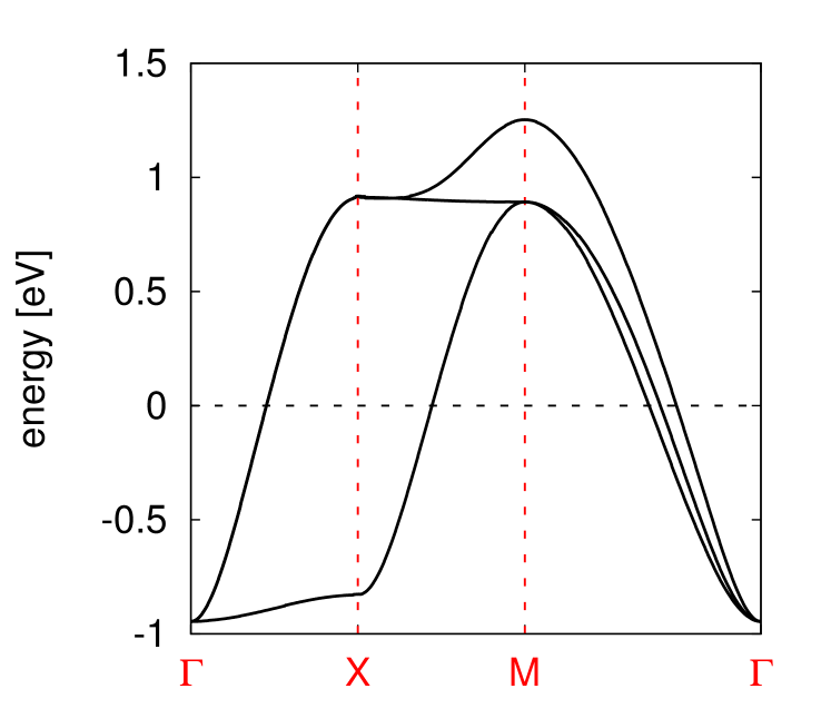
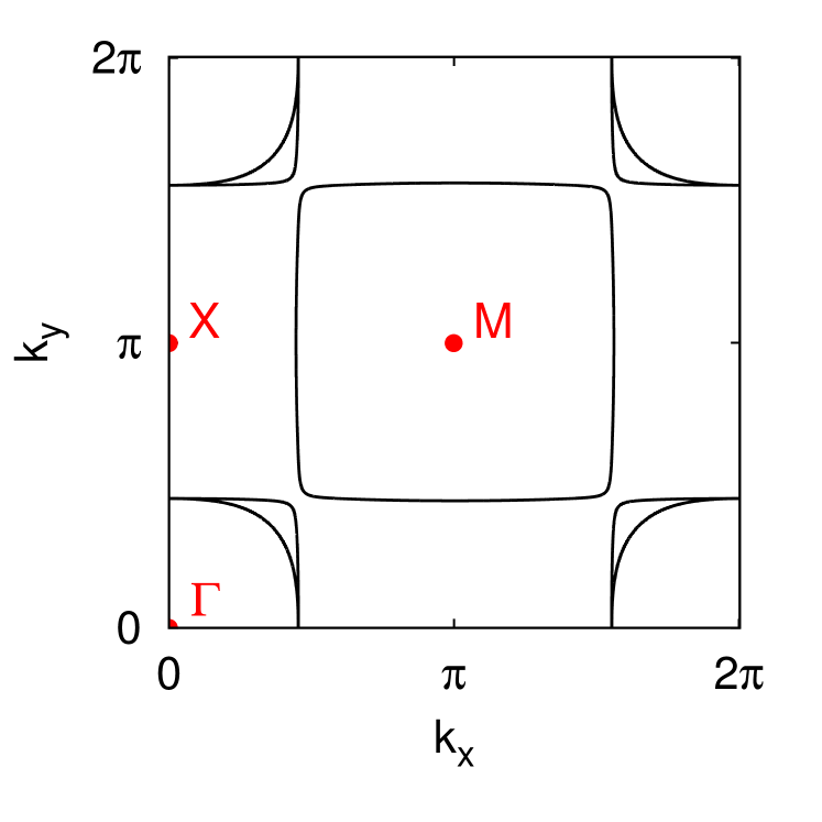
Figure 4: Bandstructure and Fermi surface of SrVO₃ within GGA: Shown is the dispersion of the vanadium $t_{2g}$ states (left) and the Fermi surface in the $(k_{x},k_{y})$-plane for $k_{z}=0$ (right).

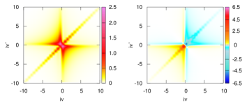
Figure 5: (Color online) Real (left) and imaginary (right) part of the generalized susceptibility $\chi_{m,1111}^{\omega\nu\nu^{\prime}}$ in the magnetic ($m$) channel for the $1111$ orbital component at $\omega=0$. $\chi$ is related to the irreducible local vertex via Eq. (30). By summing $\chi_{m}^{\omega\nu\nu^{\prime}}$ over its two fermionic frequencies $\nu$ and $\nu^{\prime}$ one can obtain the physical local magnetic susceptibility $\chi_{m}^{\omega}$, as e.g. in Ref. Galler et al., 2015.

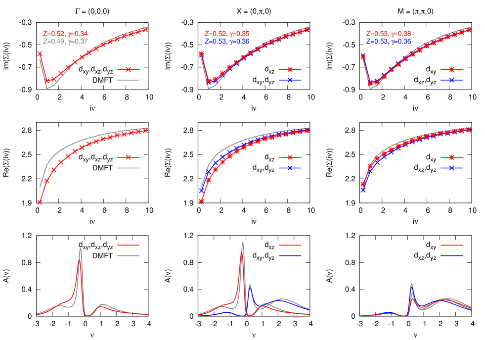
Figure 6: (Color online) AbinitioD$\Gamma$A $\mathbf{k}$-dependent self energies and spectral functions for SrVO₃. Shown are the imaginary (top) and real (middle) part of the self-energy and the corresponding spectral function (bottom) for the k-points $\Gamma=(0,0,0)$ (first column), $X=(0,\pi,0)$ (second column) and $M=(\pi,\pi,0)$ (third column).

Here we first employ Wien2K Schwarz and Blaha (2003) bandstructure calculations in the generalized gradient approximation (GGA) Perdew et al. (1996) and wien2wannier Kuneš et al. (2010) to project onto maximally localized Wannier functionsMostofi et al. (2008) for the low energy $t_{2g}$ orbitals of vanadium. The momentum dispersion corresponding to these orbitals is shown in Fig. 4 (left) along with a cut of the Fermi surface (right). For these low-energy orbitals the constrained local density approximation yields an intra-orbital Hubbard $U=5\,$eV, a Hund’s exchange $J=0.75\,$eV and an inter-orbital $U^{\prime}=U-2J=3.5\,$eV. Sekiyama et al. (2004); Nekrasov et al. (2006) These interaction values were shown to reproduce the experimental mass enhancement within DMFT.Sekiyama et al. (2004); Pavarini et al. (2004); Nekrasov et al. (2006)

We use the Kanamori parametrisation of the local interaction with the above values for $U$, $U^{\prime}$ and $J$ and perform DMFT calculations for the thus defined low-energy model at an inverse temperature $\beta=10eV^{-1}$. In DMFT the lattice model is self-consistently mapped onto an auxiliary single Anderson impurity model (SIAM).Georges et al. (1996a) In order to extract the local dynamic four-point vertex function we use the w2dynamics package,Parragh et al. (2012); Wallerberger (2016) which solves the SIAM using continuous-time quantum Monte Carlo in the hybridisation expansion (CT-HYB).Werner et al. (2006); Gull et al. (2011a) When considering non-density-density interactions (such as the Kanamori interaction), the multi-orbital vertex function is only accessible by extending CT-HYB with a worm algorithmGunacker et al. (2015). To illustrate the complexity of this quantity, we display in Fig. 5 the generalized susceptibility $\chi_{m,1111}^{\omega\nu\nu^{\prime}}$ (related to the vertex via Eq. 30) as a function of the two fermionic frequencies at zero bosonic frequency and all orbital indices being the same. We sample a cubic frequency box with 120 points in each direction. For relatively high temperatures of $\beta=10eV^{-1}$ this box is sufficiently large, although we suggest an extrapolation to an infinite frequency box for the self-energy in Eq. 61 or the use of high frequency asymptoticsKuneš (2011); Li et al. (2016); Wentzell2016 for future calculations. While the CT-HYB algorithm is in principle numerically exact, the four-point vertex function usually suffers from poor statistics due to finite computation times. In an effort to limit the statistical uncertainties to an acceptable level, we further make use of a sampling method termed “improved estimators”.Hafermann et al. (2012); Gunacker16 This method redefines Green’s function estimators of CT-HYB by employing local versions of the equation of motion, resulting in an improved high-frequency behavior for sampled quantities.

Following the AbinitioD$\Gamma$A approach developed in Sec. II, we compute the momentum-dependent self-energy $\Sigma_{mm^{\prime}}(\mathbf{k},i\nu)$ for SrVO₃ in the $t_{2g}$ subspace ($m=xy,xz,yz$). Here, we employ a one shot AbinitioD$\Gamma$A with the local vertex from a DFT+DMFT calculation (using the constrained DFT interaction) as a starting point. Concomitant to the restriction to the $t_{2g}$ subspace and the DFT starting point, we do not include the inter-site interaction $\mathbf{V}^{{\mathbf{q}}}$.

Let us note that recent $GW$+DMFT studies Tomczak et al. (2012a, 2014); Boehnke2016 suggest $t_{2g}$ spectral weight above $\sim 1.5$eV to be of plasmonic origin instead of stemming from the upper Hubbard bands seen in previous (static) DFT+DMFT calculations. To include this kind of physics one would need to use a frequency dependent $U(\omega)$ from constrained RPA (or a larger window of orbitals in AbinitioD$\Gamma$A taking at least $U$ and $\mathbf{V}^{{\mathbf{q}}}$ as a vertex as discussed in Section II), as well as non-local interactions $\mathbf{V}^{{\mathbf{q}}}$ that compete with the bandwidth-narrowing effects from $U(\omega)$ in $GW$+DMFT.Tomczak et al. (2014); NoteVSVO This goes beyond the scope of the present work, where both aspects are not included, and hence we cannot contribute to this controversy. Instead, we focus on the non-local effects stemming from a local frequency-independent $U$. These are other corrections to the DFT+DMFT description of SrVO₃.

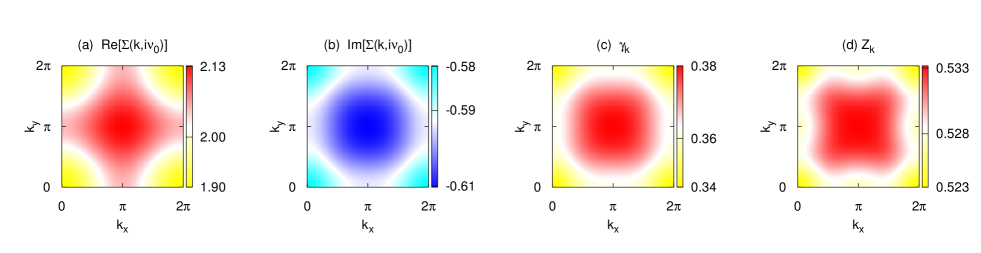
Figure 7: (Color online) (a) Real and (b) imaginary part of the AbinitioD$\Gamma$A self-energy $\Sigma(\mathbf{k},i\nu_{0})$ at the first Matsubara frequency $\nu_{0}$ (c) scattering rate $\gamma_{\mathbf{k}}$ and (d) quasiparticle weight $Z_{\mathbf{k}}$ in the $k_{z}=0$ plane for the $d_{xy}$ orbital.Note (3)

The results for the self-energy are displayed in the two top panels of Fig. 6 for three selected $\mathbf{k}$-points and are compared to the momentum-independent DMFT self-energy. We first discuss the self-energy via its low-frequency expansion: $\Sigma(\mathbf{k},i\nu)=\Re(\mathbf{k},i\nu\rightarrow 0)+i\Im\Sigma(\mathbf{k},i\nu\rightarrow 0)+(1-1/Z_{\mathbf{k}})i\nu+\mathcal{O}(\nu^{2})$. From the local DMFT self-energy we extractNote (3) a quasi-particle weight $Z^{\hbox{\tiny DMFT}}=0.49$ and a scattering rate $\gamma^{\hbox{\tiny DMFT}}\equiv-\Im\Sigma^{\hbox{\tiny DMFT}}(i\nu\rightarrow 0)=0.37\,$eV. The imaginary parts of the AbinitioD$\Gamma$A Matsubara self-energy (see Fig. 6 top panel) suggest a slight enhancement of the quasi-particle weight $Z_{\mathbf{k}}$ (smaller slope at low energy) for all momenta and orbital components. Interestingly, we find for the quasi-particle weight $Z_{\mathbf{k}}$ an extremely weak momentum-dependence. Indeed $Z_{\mathbf{k}}$ varies by less than 2% within the Brillouin zone. This is also illustrated in Fig. 7(d) which displays $Z_{\mathbf{k}}$ of the $d_{xy}$ Wannier orbital in the $k_{z}=0$ plane. The corresponding dependence of $\gamma_{\mathbf{k}}$ is displayed in panel (c) of Fig. 7. Also here, we see only a small momentum differentiation of at most 10%.

The momentum-dependence of the D$\Gamma$A self-energy in general further allows for an orbital differentiation of correlation effects in this locally degenerate system.NoteOffdiag For $Z_{\mathbf{k}}$ and $\gamma_{\mathbf{k}}$ that are both obtained from the imaginary part of the Matsubara self-energy, only a small difference between (at this $\mathbf{k}$) non-equivalent orbital components develops (see top panel in Fig. 6).

Much more sizable effects occur for both the momentum and the orbital dependence of the real-part of the self-energy at low energies. This can be inferred from the middle panel of Fig. 6 and Fig. 7 (a) that displays $\Re\Sigma(\mathbf{k},i\nu_{0})$ at the lowest Matsubara frequency, again for the $d_{xy}$ orbital in the $k_{z}=0$ plane. We witness a momentum-differentiation of 0.2eV or more—a quite notable effect beyond DMFT. We note that, contrary to $Z_{\mathbf{k}}$ and $\gamma_{\mathbf{k}}$, the momentum-dependence of $\Re\Sigma(\mathbf{k},i\nu_{0})$ in Fig. 7 (a) does not mirror the shape of the Fermi surface in Fig. 4 (right). This will in particular influence transport properties that probe states in close proximity to the Fermi surface.

At low energies, we also find a pronounced orbital-dependence in $\Re\Sigma(\mathbf{k},i\nu)$: At the $X$-point the real-part of the low-frequency self-energy is larger by about 0.1eV for the (at this $k$ point) degenerate $d_{xy}$, $d_{yz}$ orbitals than for the $d_{xz}$ component. At the $M$ point the $d_{xy}$ component is larger than the $d_{xz}$, $d_{yz}$ doublet.

Combining the influence of the orbital- and momentum dependent self-energy, we hence find systematically larger shifts $\Re\Sigma(\mathbf{k},i\nu=0)$ for excitations with higher initial (DFT) energy. Seen relatively, this means that unoccupied states are pushed upwards and occupied states downwards, resulting in a widening of the overall band-width. This was previously evidenced using perturbative techniques.Miyake et al. (2013); Tomczak (2015); Tomczak et al. (2014)

At high energies, the self-energy becomes again independent of orbital and momentum to recover the value of the Hartree term. Note (5)

We now use the maximum entropy method Jarrell and Gubernatis (1996); Sandvik (1998) to analytically continue the AbinitioD$\Gamma$A Green’s function to real frequency spectra. Let us note that, in our AbinitioD$\Gamma$A calculations we do not update the chemical potential. However, from the D$\Gamma$A Green’s function we find a particle number of 1.062, which is very close to the target occupation of 1.

In the lowest panel of Fig. 6 we compare our results to conventional DMFT for selected k-points. From the above discussion it is clear that the AbinitioD$\Gamma$A self-energy will cause quantitative differences in the many-body spectra, while the overall shape will be qualitatively similar to our and previous DMFT results. As evidenced above, the inclusion of non-local fluctuations decreases the degree of electronic correlations: Both a larger $Z$ and the shifts induced by $\Re\Sigma$ slightly increase the interacting band-width with respect to DMFT. Indeed we see in our spectra signatures of reduced correlations: Hubbard bands are less pronounced and quasi-particle peaks move away from the Fermi level, although in the current case these effects are small. This is congruent with previous dynamical cluster approximation (DCA) calculations that included short-ranged non-local fluctuations.Lee et al. (2012) Let us also note that recently it was indeed found experimentally,Backes et al. (2016) that the lower Hubbard band in SrVO₃ is intrinsically somewhat less pronounced than previously thought, with a substantial part of spectral weight actually originating from oxygen vacancies.

The very weak momentum dependence of the quasi-particle dynamics and electronic lifetimes does not come as a surprise. Indeed the local nature of $Z$ was previously established in a D$\Gamma$A study of the 3D Hubbard modelSchäfer et al. (2015), and, using perturbative techniques, in metallic oxidesTomczak et al. (2014) and the iron pnictides and chalcogenidesTomczak et al. (2012b); Tomczak (2015). On the other hand, these studies found a largely momentum-dependent static contribution $\Re\Sigma(\mathbf{k},\nu=0)$ to the self-energy. Going beyond model studies and perturbative methods, we here confirm that $\Re\Sigma(\mathbf{k},\nu=0)$ indeed contains non-negligible momentum-dependent correlations beyond DMFT even for only purely local interactions. Still, in the current study, momentum-dependent effects are small enough to only lead to quantitative changes. There are three main reasons for the preponderance of local self-energy effects: (1) SrVO₃ is not in close proximity to a spin-ordered phase or any other second order phase transitions. Therefore, non-local spin- or charge-fluctuations were not expected to be particularly strong. (2) SrVO₃ is a cubic, i.e. fairly isotropic system. Non-local correlation effects are generally more pronounced in anisotropic or lower dimensional systems. Therefore, we can speculate that non-local self-energies will become more prevalent in ultra-thin films of SrVO₃Yoshimatsu et al. (2010); Zhong et al. (2015). (3) The $GW$ approach in fact yields a much larger static $\mathbf{k}$-dependence $\Re\Sigma(\mathbf{k},\nu=0)$.Miyake et al. (2013); Tomczak et al. (2014) This is however an effect of the non-locality of the interaction which yields a largely momentum-dependent screened exchange contribution to the self-energy. Note (7) While non-local interactions are included in the AbinitioD$\Gamma$A formalism (see Sec. II), we here performed calculations with a local interaction only, and are thus missing this effect.

IV Conclusion and outlook

In conclusion we have derived, implemented, and applied a new first principles technique for correlated materials: the AbinitioD$\Gamma$A approach. The method is a diagrammatic extension of the successful DMFT approximation and treats electronic correlation effects on all time and length scales. Since it includes the self-energy diagrams of DMFT, the GW approach and non-local correlations beyond both, we believe AbinitioD$\Gamma$A to set a new standard in realistic many-body calculations. We first applied the new methodology to the transition metal oxide SrVO₃ in a one-shot setup and neglected the influence of frequency dependent and non-local interactions, $U(\omega)$ and $V^{q}$, respectively. Consequently the plasmonic physics recently reported in $GW$+DMFTTomczak et al. (2012a, 2014); Boehnke2016 is not included. Here we focused on non-local correlation effects beyond DFT+DMFT that arise from a purely local Hubbard-like interaction such as non-local spin fluctuations.

We find that while the quasi-particle weight $Z$ is essentially local, there is a notable momentum- and orbital-dependence in the real part of the self-energy. We hence conclude that non-local correlations can be important even in fairly isotropic systems in three dimensions, in the absence of any fluctuations associated with a nearby ordered phase, and can occur even for purely local (Hubbard & Hund) interactions. These findings herald the need for advancing state-of-the-art methodologies for the many-body problem. In this vein, AbinitioD$\Gamma$A presents a very promising route toward the quantitative simulation of materials. In future studies the approach can be applied to systems in which non-local fluctuations play a greater role, such as compounds in proximity to second order phase transitions or lower dimensional systems. For such materials non-local correlations beyond DMFT are a journey into the unknown.

Acknowledgments. We thank J. Kaufmann, G. Rohringer, T. Schäfer and A. Toschi for useful discussions, as well as A. Sandvik for making available his maximum entropy program. This work has been supported by European Research Council under the European Union’s Seventh Framework Program (FP/2007-2013)/ERC through grant agreement n. 306447; AG also thanks the Doctoral School W1243 Solids4Fun (Building Solids for Function) of the Austrian Science Fund (FWF). Calculations have been done on the Vienna Scientific Cluster (VSC).

Note added. In the course of finalizing this work, we became aware of the independent development of a related ab initio vertex approach by Nomura et al. Y. Nomura et al. based on another diagrammatic DMFT extension, the triply-irreducible local expansion akin to D$\Gamma$A.

References

- Hohenberg and Kohn (1964) P. Hohenberg and W. Kohn, Phys. Rev. 136, B864 (1964).
- Kohn and Sham (1965) W. Kohn and L. Sham, Phys. Rev. 140, (4A) A1133 (1965).
- Jones and Gunnarsson (1989) R. Jones and O. Gunnarsson, Rev. Mod. Phys. 61, 689 (1989).
- Martin et al. (2004) R. M. Martin, L. Reining, and D. M. Ceperley, Interacting Electrons: Theory and Computational Approaches (Cambridge University Press Cambridge, 2004).
- Martin (2016) R. M. Martin, Electronic Structure: Basic Theory and Practical Methods (Cambridge University Press Cambridge, 2016).
- Hedin (1965) L. Hedin, Phys. Rev. 139, A796 (1965).
- Metzner and Vollhardt (1989) W. Metzner and D. Vollhardt, Phys. Rev. Lett. 62, 324 (1989).
- Georges and Kotliar (1992) A. Georges and G. Kotliar, Phys. Rev. B 45, 6479 (1992).
- Georges et al. (1996a) A. Georges, G. Kotliar, W. Krauth, and M. J. Rozenberg, Rev. Mod. Phys. 68, 13 (1996a).
- Anisimov et al. (1997) V. I. Anisimov, A. I. Poteryaev, M. A. Korotin, A. O. Anokhin, and G. Kotliar, Journal of Physics: Condensed Matter 9, 7359 (1997).
- Lichtenstein and Katsnelson (1998) A. I. Lichtenstein and M. I. Katsnelson, Phys. Rev. B 57, 6884 (1998).
- Kotliar et al. (2006) G. Kotliar, S. Y. Savrasov, K. Haule, V. S. Oudovenko, O. Parcollet, and C. A. Marianetti, Rev. Mod. Phys. 78, 865 (2006).
- Held (2007) K. Held, Advances in Physics 56, 829 (2007).
- Biermann et al. (2003) S. Biermann, F. Aryasetiawan, and A. Georges, Phys. Rev. Lett. 90, 086402 (2003).
- Tomczak et al. (2012a) J. M. Tomczak, M. Casula, T. Miyake, F. Aryasetiawan, and S. Biermann, EPL (Europhysics Letters) 100, 67001 (2012a).
- Taranto et al. (2013) C. Taranto, M. Kaltak, N. Parragh, G. Sangiovanni, G. Kresse, A. Toschi, and K. Held, Phys. Rev. B 88, 165119 (2013).
- Sakuma et al. (2013) R. Sakuma, P. Werner, and F. Aryasetiawan, Phys. Rev. B 88, 235110 (2013).
- Tomczak et al. (2014) J. M. Tomczak, M. Casula, T. Miyake, and S. Biermann, Phys. Rev. B 90, 165138 (2014).
- Tomczak (2015) J. M. Tomczak, Journal of Physics: Conference Series 592, 012055 (2015), preprint arXiv:1411.5180.
- Choi et al. (2016) S. Choi, A. Kutepov, K. Haule, M. van Schilfgaarde, and G. Kotliar, Npj Quantum Materials 1, 16001 EP (2016).
- (21) L. Boehnke, F. Nilsson, F. Aryasetiawan, and P. Werner, Phys. Rev. B 94 201106 (2016).
- (22) An interesting alternative is also to combine screened exchange and DMFT, see Roekeghem2014_1 ; Roekeghem2014_2 .
- (23) A. van Roekeghem, T. Ayral, J. M. Tomczak, M. Casula, N. Xu, H. Ding, M. Ferrero, O. Parcollet, H. Jiang, and Silke Biermann Phys. Rev. Lett. 113, 266403 (2014).
- (24) A. van Roekeghem and Silke Biermann, EPL (Europhysics Letters) 108, 57003 (2014).
- Si and Smith (1996a) Si, Q, and J. L. Smith (1996a),Phys. Rev. Lett. 77, 3391.
- Chitra and Kotliar (2000) Chitra, R, and G. Kotliar (2000),Phys. Rev. Lett. 84, 3678–3681.
- Kusunose (2006) H. Kusunose, J. Phys. Soc. Jpn 75, 054713 (2006).
- Toschi et al. (2007) A. Toschi, A. A. Katanin, and K. Held, Phys. Rev. B 75, 045118 (2007).
- Katanin et al. (2009) A. A. Katanin, A. Toschi, and K. Held, Phys. Rev. B 80, 075104 (2009).
- Rubtsov et al. (2008) A. N. Rubtsov, M. I. Katsnelson, and A. I. Lichtenstein, Phys. Rev. B 77, 033101 (2008).
- Slezak et al. (2009) C. Slezak, J. M., T. Maier, and J. Deisz, J. Phys.: Condens. Matter 21, 435604 (2009).
- Rohringer et al. (2013) G. Rohringer, A. Toschi, H. Hafermann, K. Held, V. I. Anisimov, and A. A. Katanin, Phys. Rev. B 88, 115112 (2013).
- Taranto et al. (2014) C. Taranto, S. Andergassen, J. Bauer, K. Held, A. Katanin, W. Metzner, G. Rohringer, and A. Toschi, Phys. Rev. Lett. 112, 196402 (2014).
- Kitatani et al. (2015) M. Kitatani, N. Tsuji, and H. Aoki, Phys. Rev. B 92, 085104 (2015).
- Ayral and Parcollet (2015) T. Ayral and O. Parcollet, Phys Rev. B 92, 115109 (2015).
- Li (2015) G. Li, Phys. Rev. B 91, 165134 (2015).
- Valli et al. (2015) A. Valli, T. Schäfer, P. Thunström, G. Rohringer, S. Andergassen, G. Sangiovanni, K. Held, and A. Toschi, Phys. Rev. B 91, 115115 (2015).
- Li et al. (2016) G. Li, N. Wentzell, P. Pudleiner, P. Thunström, and K. Held, Phys. Rev. B 93, 195134 (2016).
- Rohringer et al. (2011) G. Rohringer, A. Toschi, A. Katanin, and K. Held, Phys. Rev. Lett. 107, 256402 (2011).
- Antipov et al. (2014) A. E. Antipov, E. Gull, and S. Kirchner, Phys. Rev. Lett. 112, 226401 (2014).
- Hirschmeier et al. (2015) D. Hirschmeier, H. Hafermann, E. Gull, A. I. Lichtenstein, and A. E. Antipov, Phys. Rev. B 92, 144409 (2015).
- Schäfer et al. (2016) T. Schäfer, A. Katanin, K. Held, and A. Toschi, preprint arXiv:1605.06355 (2016) .
- Schäfer et al. (2015) T. Schäfer, A. Toschi, and J. M. Tomczak, Phys. Rev. B 91, 121107 (2015).
- (44) See however Refs. Takada, 2001; Stefanucci et al., 2014; Kutepov, 2016 for including selected vertex corrections within the GW formalism.
- Toschi et al. (2011) A. Toschi, G. Rohringer, A. Katanin, and K. Held, Annalen der Physik 523, 698 (2011).
- Katanin (2016) A. A. Katanin, preprint arXiv:1604.01702 (2016) .
- Rubtsov et al. (2012) A. N. Rubtsov, M. I. Katsnelson, and A. I. Lichtenstein, Ann. Phys. 327, 1320 (2012).
- Andersen and Saha-Dasgupta (2000) O. K. Andersen and T. Saha-Dasgupta, Phys. Rev. B 62, R16219 (2000).
- Kuneš et al. (2010) J. Kuneš, R. Arita, P. Wissgott, A. Toschi, H. Ikeda, and K. Held, Computer Physics Communications 181, 1888 (2010).
- Mostofi et al. (2008) A. A. Mostofi, J. R. Yates, Y.-S. Lee, I. Souza, D. Vanderbilt, and N. Marzari, Comput. Phys. Commun. 178, 685 (2008).
- (51) P. H. Dederichs, S. Blügel, R. Zeller and H. Akai, Phys. Rev. Lett. 53 2512 (1984).
- (52) A. K. McMahan, R. M. Martin and S. Satpathy, Phys. Rev. B 38 6650 (1988).
- (53) O. Gunnarsson, O. K. Andersen, O. Jepsen and J. Zaanen, Phys. Rev. B 39 1708 (1989).
- Aryasetiawan et al. (2004) F. Aryasetiawan, M. Imada, A. Georges, G. Kotliar, S. Biermann, and A. I. Lichtenstein, Phys. Rev. B 70, 195104 (2004).
- Miyake and Aryasetiawan (2008) T. Miyake and F. Aryasetiawan, Phys. Rev. B 77, 085122 (2008).
- Tomczak et al. (2010) J.M. Tomczak, T. Miyake and F. Aryasetiawan, Phys. Rev. B 81, 115116 (2010).
- Gull et al. (2011a) E. Gull, A. J. Millis, A. I. Lichtenstein, A. N. Rubtsov, M. Troyer, and P. Werner, Rev. Mod. Phys. 83, 349 (2011a).
- (58) L. Boehnke, A. I. Lichtenstein, M. I. Katsnelson, F. Lechermann, arXiv:1407.4795.
- Gunacker et al. (2015) P. Gunacker, M. Wallerberger, E. Gull, A. Hausoel, G. Sangiovanni, and K. Held, Phys. Rev. B 92, 155102 (2015).
- (60) P. Gunacker, M. Wallerberger, T. Ribic, A. Hausoel, G. Sangiovanni, and K. Held Phys. Rev. B 94, 125153 (2016).
- Held et al. (2008) K. Held, A. Katanin, and A. Toschi, Progress of Theoretical Physics (Supplement) 176, 117 (2008).
- Held (2014) K. Held, Lecture Notes ”Autumn School on Correlated Electrons. DMFT at 25: Infinite Dimensions”, Reihe Modeling and Simulation, Vol. 4, Forschungszentrum Juelich GmbH (publisher) [arXiv:1411.5191] (2014).
- Ayral and Parcollet (2016) T. Ayral and O. Parcollet, Phys. Rev. B 94, 075159 (2016) .
- (64) S. Y. Savrasov and G. Kotliar, Phys. Rev. B 69, 245101 (2004).
- (65) J. Minár, L. Chioncel, A. Perlov, H. Ebert, M. I. Katsnelson, and A. I. Lichtenstein, Phys. Rev. B 72, 045125 (2005).
- (66) L. V. Pourovskii, B. Amadon, S. Biermann, and A. Georges Phys. Rev. B 76, 235101 (2007).
- (67) M. Aichhorn, L. Pourovskii, and A. Georges Phys. Rev. B 84, 054529 (2011).
- (68) S. Bhandary, E. Assmann, M. Aichhorn, and K. Held, Phys. Rev. B 94, 155131 (2016).
- (69) S. V. Faleev, M. van Schilfgaarde, and T. Kotani, Phys. Rev. Lett. 93, 126406 (2004).
- (70) A. N. Chantis, M. van Schilfgaarde, and T. Kotani, Phys. Rev. Lett. 96, 086405 (2006).
- (71) Beyond , which only includes the particle-hole channel, also the diagrams of the particle-hole transversal channel are included. Moreover, in only the first term of Fig. 2 (b) is included, not the crossed which describes spin fluctuations. At least for the local part of the less correlated orbitals this crossed term can be included with ease, as it is independent of . It corresponds to having a different vertex for spin and charge contributions (see below). Such a combined scheme where the local vertex is calculated for some correlated orbitals and is taken for the less correlated orbitals is best combined with a treatment to avoid double counting self-energies.
- (72) For a related strategy within the GW formalism, see Ref. Hirayama, .
- (73) M. Hirayama, T. Miyake, and M. Imada, Phys. Rev. B 87, 195144 (2013).
- Schaefer et al. (2016) T. Schäfer, S. Ciuchi, M. Wallerberger, P. Thunström, O. Gunnarsson, G. Sangiovanni, G. Rohringer, and A. Toschi, Phys. Rev. B 94, 235108 (2016) .
- Hafermann et al. (2012) H. Hafermann, K. R. Patton, and P. Werner, Phys. Rev. B 85, 205106 (2012).
- Sekiyama et al. (2004) A. Sekiyama, H. Fujiwara, S. Imada, S. Suga, H. Eisaki, S. I. Uchida, K. Takegahara, H. Harima, Y. Saitoh, I. A. Nekrasov, G. Keller, D. E. Kondakov, A. V. Kozhevnikov, T. Pruschke, K. Held, D. Vollhardt, and V. I. Anisimov, Phys. Rev. Lett. 93, 156402 (2004).
- Inoue et al. (1998) I. H. Inoue, O. Goto, H. Makino, N. E. Hussey, and M. Ishikawa, Phys. Rev. B 58, 4372 (1998).
- Nekrasov et al. (2006) I. A. Nekrasov, K. Held, G. Keller, D. E. Kondakov, T. Pruschke, M. Kollar, O. K. Andersen, V. I. Anisimov, and D. Vollhardt, Phys. Rev. B 73, 155112 (2006).
- Byczuk et al. (2007) K. Byczuk, M. Kollar, K. Held, Y.-F. Yang, I. A. Nekrasov, T. Pruschke, and D. Vollhardt, Nature Physics 3, 168 (2007).
- Aizaki et al. (2012) S. Aizaki, T. Yoshida, K. Yoshimatsu, M. Takizawa, M. Minohara, S. Ideta, A. Fujimori, K. Gupta, P. Mahadevan, K. Horiba, H. Kumigashira, and M. Oshima, Phys. Rev. Lett. 109, 056401 (2012).
- Held et al. (2013) K. Held, R. Peters, and A. Toschi, Phys. Rev. Lett. 110, 246402 (2013).
- Pavarini et al. (2004) E. Pavarini, S. Biermann, A. Poteryaev, A. I. Lichtenstein, A. Georges, and O. K. Andersen, Phys. Rev. Lett. 92, 176403 (2004).
- Lee et al. (2012) H. Lee, K. Foyevtsova, J. Ferber, M. Aichhorn, H. O. Jeschke, and R. Valentí, Phys. Rev. B 85, 165103 (2012).
- Casula et al. (2012) M. Casula, A. Rubtsov, and S. Biermann, Phys. Rev. B 85, 035115 (2012).
- Miyake et al. (2013) T. Miyake, C. Martins, R. Sakuma, and F. Aryasetiawan, Phys. Rev. B 87, 115110 (2013).
- Nakamura et al. (2016) K. Nakamura, Y. Nohara, Y. Yosimoto, and Y. Nomura, Phys. Rev. B 93, 085124 (2016).
- Moyer et al. (2013) J. A. Moyer, C. Eaton, and R. Engel-Herbert, Advanced Materials 25, 3578 (2013).
- Zhong et al. (2015) Z. Zhong, M. Wallerberger, J. M. Tomczak, C. Taranto, N. Parragh, A. Toschi, G. Sangiovanni, and K. Held, Phys. Rev. Lett. 114, 246401 (2015), preprint arXiv:1312.5989.
- Zhang et al. (2016) L. Zhang, Y. Zhou, L. Guo, W. Zhao, A. Barnes, H.-T. Zhang, C. Eaton, Y. Zheng, M. Brahlek, H. F. Haneef, N. J. Podraza, M. H. W. Chan, V. Gopalan, K. M. Rabe, and R. Engel-Herbert, Nat Mater 15, 204 (2016), article.
- Galler et al. (2015) A. Galler, C. Taranto, M. Wallerberger, M. Kaltak, G. Kresse, G. Sangiovanni, A. Toschi, and K. Held, Phys. Rev. B 92, 205132 (2015).
- Schwarz and Blaha (2003) K. Schwarz and P. Blaha, Comp. Mater. Sci. 28, 259 (2003).
- Perdew et al. (1996) J. P. Perdew, K. Burke, and M. Ernzerhof, Phys. Rev. Lett. 77, 3865 (1996).
- Parragh et al. (2012) N. Parragh, A. Toschi, K. Held, and G. Sangiovanni, Phys. Rev. B 86, 155158 (2012).
- Wallerberger (2016) M. Wallerberger, PhD Thesis (TU Wien, 2016).
- Werner et al. (2006) P. Werner, A. Comanac, L. de’ Medici, M. Troyer, and A. J. Millis, Phys. Rev. Lett. 97, 076405 (2006).
- Kuneš (2011) J. Kuneš, Phys. Rev. B 83, 085102 (2011).
- (97) N. Wentzell, G. Li, A. Tagliavini, C. Taranto, G. Rohringer, K. Held, A. Toschi, and S. Andergassen, arXiv:1610.06520.
- (98) Our constrained RPA estimate yields the following interactions for the maximally localized Wannier setup: local Hubbard interaction eV, nearest neighbor interaction eV, next-nearest neighbor interaction eV. Note that this constrained RPA value for taken at is smaller than the constrained DFT value employed in our calculation, which can be understood from the fact that ) increases with so that a larger static is necessary to arrive at a similar level of correlation.
- Note (3) We extract the expansion coefficients from the Matsubara data with a 3rd-order polynomial fit to at the first six Matsubara frequencies, and limit the discussion to orbital-diagonal components. The expansion coefficients determined this way should be taken with a grain of salt: Given the rather high temperature (eV-1) we are not yet clearly in the linear regime to determine with high accuracy, not to speak of the kink in Nekrasov et al. (2006); Byczuk et al. (2007) as an additional complication (because of the temperature, our crude estimate rather corresponds to the high energy after the kink). Spectra are computed with the full self-energy.
- (100) In particular, away from high-symmetry points, the lifting of degeneracy also allows for orbital-offdiagonal components in the self-energy. We however find these to be very small in the current system, which is why we limit the discussion to the diagonal components.
- Note (5) The Hartree term is -independent since the interactions we use are local.
- Jarrell and Gubernatis (1996) M. Jarrell and J. E. Gubernatis, Physics Reports 269, 133 (1996).
- Sandvik (1998) A. W. Sandvik, Phys. Rev. B 57, 10287 (1998).
- Backes et al. (2016) S. Backes, T. C. Rödel, F. Fortuna, E. Frantzeskakis, P. Le Fèvre, F. Bertran, M. Kobayashi, R. Yukawa, T. Mitsuhashi, M. Kitamura, K. Horiba, H. Kumigashira, R. Saint-Martin, A. Fouchet, B. Berini, Y. Dumont, A. J. Kim, F. Lechermann, H. O. Jeschke, M. J. Rozenberg, R. Valentí, and A. F. Santander-Syro, Phys. Rev. B 94, 241110(R) (2016) .
- Tomczak et al. (2012b) J. M. Tomczak, M. van Schilfgaarde, and G. Kotliar, Phys. Rev. Lett. 109, 237010 (2012b), preprint arXiv:1209.2213.
- Yoshimatsu et al. (2010) K. Yoshimatsu, T. Okabe, H. Kumigashira, S. Okamoto, S. Aizaki, A. Fujimori, and M. Oshima, Phys. Rev. Lett. 104, 147601 (2010).
- Note (7) Indeed, applying the approach to the one-band Hubbard model (in which exchange effects are absent by construction), results in a negligible momentum dependence of in three dimensions, see Ref \rev@citealpnumSchaefer2015.
- (108) Y. Nomura et al., unpublished.
- Takada (2001) Y. Takada, Phys. Rev. Lett. 87, 226402 (2001).
- Stefanucci et al. (2014) G. Stefanucci, Y. Pavlyukh, A.-M. Uimonen, and R. van Leeuwen, Phys. Rev. B 90, 115134 (2014).
- Kutepov (2016) A. L. Kutepov, Phys. Rev. B 94, 155101 (2016).