Distributed Convex Optimization with Many Non-Linear Constraints

Abstract

We address the problem of solving convex optimization problems with many non-linear constraints in a distributed setting. Our approach is based on an extension of the alternating direction method of multipliers (ADMM). Although it has been invented decades ago, ADMM so far can be applied only to unconstrained problems and problems with linear equality or inequality constraints. Our extension can directly handle arbitrary inequality constraints. It combines the ability of ADMM to solve convex optimization problems in a distributed setting with the ability of the Augmented Lagrangian method to solve constrained optimization problems, and as we show, it inherits the convergence guarantees of both ADMM and the Augmented Lagrangian method.

1 Introduction

The increasing availability of distributed hardware suggests addressing large scale optimization problems by distributed algorithms. Large scale optimization problems involve a large number of optimization variables, or a large number of input parameters, or a large number of constraints. Here we address the latter case of a large number of constraints.

In recent years, the alternating direction method of multipliers (ADMM) that was proposed by Glowinski and Marroco [9] and by Gabay and Mercier [7] already decades ago obtained considerable attention, also beyond the machine learning community, because it allows to solve convex optimization problems that involve a large number of parameters in a distributed setting [2]. For instance, the parameters in ordinary least squares regression are just the data points. The optimization problem behind a typical machine learning method usually aims for minimizing a loss-function that is the sum of the losses for each data point. Hence, the objective function $f$ of such problems is separable, i.e., it holds that $f(x)=\sum_{i}f_{i}(x_{i})$, where $f_{i}$ is determined by the $i$-th data point. In this case ADMM lends itself to a distributed implementation where the data points are distributed on different compute nodes.

Standard ADMM works for unconstrained optimization problems and for optimization problems with linear equality and/or inequality constraints. Surprisingly, so far no general convex inequality constraints have been considered directly in the context of ADMM. Optimization problems with a large number of constraints typically also arise as big data problems, but instead of contributing a term to the objective function, each data point now contributes a constraint to the problem. An illustrative example is the core vector machine [25, 26], where the smallest enclosing ball for a given set of data points has to be computed. The objective function here is the radius of the ball that needs to be minimized, and every data point contributes a non-linear constraint, namely the distance of the point from the center must be at most the radius. Another example problem are robust SVMs that we discuss in more detail later in the paper.

In principle, standard ADMM can also be used for solving constrained optimization problems. A distributed implementation of the straightforward extension of ADMM leads to non-trivial constrained optimization subproblems that have to be solved in every iteration. Solving constrained problems is typically transformed into a sequence of unconstrained problems. Hence, this approach features three nested loops, the outer loop for reaching consensus, one loop for the constraints, and an inner loop for solving unconstrained problems. Alternatively, one could use the standard Augmented Lagrangian method, originally known as the method of multipliers[12], that has been specifically designed for solving constrained optimization problems. Combining the Augmented Lagrangian method with ADMM allows to solve general constrained problems in a distributed fashion by running the Augmented Lagrangian method in an outer loop and ADMM in an inner loop. Again, we end up with three nested loops, the outer loop for the augmented Lagrangian method and the standard two nested inner loops for ADMM. Thus, one could assume that any distributed solver for constrained optimization problems needs at least three nested loops: one for reaching consensus, one for the constraints, and one for the unconstrained problems. The key contribution of our paper is showing that this is not the case. One of the nested loops can be avoided by merging the loops for reaching consensus and dealing with the constraints. Our approach, that only needs two nested loops, combines ADMM with the Augmented Lagrangian method differently than the direct approach of running the Augmented Lagrangian method in the outer and ADMM in the inner loop. But the latter combination still provides us with a good baseline to compare against.

Related work.

To the best of our knowledge, our extension of ADMM is the first distributed algorithm for solving general convex optimization problems with no restrictions on the type of constraints or assumptions on the structure of the problem. Surprisingly, even our baseline method of running the augmented Lagrangian method in an outer loop and ADMM in an inner loop has not been studied before. The only special case, that we are aware of, are quadratically constrained quadratic problems that have been addressed by Huang and Sidiropoulos [14] using consensus ADMM. However, their approach does not scale to many constraints, because every constraint gives rise to a new subproblem.

Mosk-Aoyama et al. [18] have designed and analyzed a distributed algorithm for solving convex optimization problems with separable objective function and linear equality constraints. Their algorithm blends a gossip-based information spreading, iterative gradient ascent method with the barrier method from interior-point algorithms. It is similar to ADMM and can also handle only linear constraints.

Zhu and Martínez [29] have introduced a distributed multi-agent algorithm for minimizing a convex function that is the sum of local functions subject to a global equality or inequality constraint. Their algorithm involves projections onto local constraint sets that are usually as hard to compute as solving the original problem with general constraints. For instance, it is well known via standard duality theory that the feasibility problem for linear programs is as hard as solving linear programs. This holds true for general convex optimization problems with vanishing duality gap.

In principle, the standard ADMM can also handle convex constraints by transforming them into indicator functions that are added to the objective function. However, this leads to subproblems that need to be solved in each iteration that entail computing a projection onto the feasible region. This entails the same issues as the method by Zhu and Martínes [29] since computing these projections can be as hard as solving the original problem. We will elaborate on this in more detail in Section 3.

The recent literature on ADMM is vast. Most papers on ADMM stay in the standard framework of optimizing a function or a sum of functions subject to linear constraints and make contributions to one or more of the following aspects: (1) Theoretical (and practical) convergence guarantees [6, 10, 11, 13, 19], (2) convergence guarantees for asynchronous ADMM [27], (3) splitting the problem into more than two subproblems [4, 15], (4) optimal penalty parameter selection [8], (5) solving the individual subproblems efficiently or inexactly while still guaranteeing convergence [3, 5, 16, 21], and (6) applications of ADMM.

2 Alternating direction method of multipliers

Here, we briefly review the alternating direction method of multipliers (ADMM) and discuss how it can be adapted to deal with distributed data. ADMM is an iterative algorithm that in its most general form can solve convex optimization problems of the form

$$\begin{array}[]{cl}\min_{x,z}&f_{1}(x)+f_{2}(z)\\ \operatorname{\textrm{s.t.}}&Ax+Bz-c=0,\end{array}$$ (1)

where $f_{1}:\mathbb{R}^{n_{1}}\to\mathbb{R}\cup\{\infty\}$ and $f_{2}:\mathbb{R}^{n_{2}}\to\mathbb{R}\cup\{\infty\}$ are convex functions, $A\in\mathbb{R}^{m\times n_{1}}$ and $B\in\mathbb{R}^{m\times n_{2}}$ are matrices, and $c\in\mathbb{R}^{m}$.

ADMM can obviously deal with linear equality constraints, but it can also handle linear inequality constraints. The latter are reduced to linear equality constraints by replacing constraints of the form $Ax\leq b$ by $Ax+s=b$, adding the slack variable $s$ to the set of optimization variables, and setting $f_{2}(s)=\mathbbm{1}_{\mathbb{R}_{+}^{m}}(s)$, where

$$\mathbbm{1}_{\mathbb{R}_{+}^{m}}(s)=\begin{cases}0,&\text{if }s\geq 0\\ \infty,&\text{otherwise},\end{cases}$$

is the indicator function of the set $\mathbb{R}_{+}^{m}=\{x\in\mathbb{R}^{m}|x\geq 0\}$. Note that $f_{1}$ and $f_{2}$ are allowed to take the value $\infty$.

Recently, ADMM regained a lot of attention, because it allows to solve problems with separable objective function in a distributed setting. Such problems are typically given as

$$\begin{array}[]{cl}\min_{x}&\sum_{i}f_{i}(x),\end{array}$$

where $f_{i}$ corresponds to the $i$-th data point (or more generally $i$-th data block) and $x$ is a weight vector that describes the data model. This problem can be transformed into an equivalent optimization problem, with individual weight vectors $x_{i}$ for each data point (data block) that are coupled through an equality constraint,

$$\begin{array}[]{cl}\min_{x_{i},z}&\sum_{i}f_{i}(x_{i})\\ \operatorname{\textrm{s.t.}}&x_{i}-z=0\quad\forall\,i,\end{array}$$

which is a special case of Problem 1 that can be solved by ADMM in a distributed setting by distributing the data.

Adding convex inequality constraints to Problem 1 does not destroy convexity of the problem, but so far ADMM cannot deal with such constraints. Note that the problem only remains convex, if all equality constraints are induced by affine functions. That is, we cannot add convex equality constraints in general without destroying convexity.

Our goal for the following sections is extending ADMM such that it can also deal with nonlinear, convex inequality constraints. For problems with many constraints we will show that these constraints can be distributed similarly as the data points in problems with separable objective function are distributed for the standard ADMM.

3 Problems with non-linear constraints

We consider convex optimization problems of the form

$$\begin{array}[]{cl}\min_{x,z}&f_{1}(x)+f_{2}(z)\\ \operatorname{\textrm{s.t.}}&g_{0}(x)\leq 0\\ &h_{1}(x)+h_{2}(z)=0,\end{array}$$ (2)

where $f_{1}$ and $f_{2}$ are as in Problem 1, $g_{0}:\mathbb{R}^{n_{1}}\to\mathbb{R}^{p}$ is convex in every component, and $h_{1}:\mathbb{R}^{n_{1}}\to\mathbb{R}^{m}$ and $h_{2}:\mathbb{R}^{n_{2}}\to\mathbb{R}^{m}$ are affine functions. In the following we assume that the problem is feasible, i.e., that a feasible solution exists, and that strong duality holds. A sufficient condition for strong duality is that the interior of the feasible region is non-empty. This condition is known as Slater’s condition for convex optimization problems [24].

As stated before, our goal is extending ADMM such that it can also solve Problem 2. The simple trick of adding non-negative slack variables only works, if the constraints $g_{0}(x)\leq 0$ are affine. Still, this trick gives some insight into the general problem. We have dealt with the non-negativity constraints on the slack variables by adding an indicator function to the objective function. The indicator function forces ADMM to project the solution in every iteration onto the set $\{s\in\mathbb{R}^{m}|s\geq 0\}$ which is just the non-negative orthant. Projecting onto the non-negative orthant is an easy problem and thus ADMM can efficiently deal with linear inequality constraints. As we have already mentioned in the introduction the idea of transforming the constraints into indicator functions and adding them to the objective function can be generalized to non-linear constraints. However, ADMM then needs to compute in every iteration a projection onto the more complicated feasible set $\{x\,|\,g_{0}(x)\leq 0\}$. Such a projection is the solution to the following constrained optimization problem

$$\begin{array}[]{cl}\min_{x}&\|x\|^{2}\\ \operatorname{\textrm{s.t.}}&g_{0}(x)\leq 0,\end{array}$$

whose solving, depending on the constraints, requires a QP, SOCP or even SDP solver. Thus we have only deferred the difficulties that have been induced by the non-linear constraints to the subproblem of computing the projections. Here, we will devise a method for dealing with arbitrary constraints directly without any hard-to-compute projections.

4 ADMM extension

For our extension of ADMM and its convergence analysis we need to work with an equivalent reformulation of Problem 2, where we replace $g_{0}(x)$ by

$$g(x)=\max\{0,\,g_{0}(x)\}^{2},$$

with componentwise maximum, and turn the convex inequality constraints into convex equality constraints. Thus, in the following we consider optimization problems of the form

$$\begin{array}[]{cl}\min_{x,z}&f_{1}(x)+f_{2}(z)\\ \operatorname{\textrm{s.t.}}&g(x)=0\\ &h_{1}(x)+h_{2}(z)=0,\end{array}$$ (3)

where $g(x)=\max\{0,\,g_{0}(x)\}^{2}$, which by construction is again convex in every component and differentiable if $g(x)$ is differentiable. Note, though, that the constraint $g(x)=0$ is no longer affine. However, we show in the following that Problem 3 can still be solved efficiently.

Analogously to ADMM our extension builds on the Augmented Lagrangian for Problem 3 which is the following function

$$L_{\rho}(x,z,\mu,\lambda) =f_{1}(x)+f_{2}(z)+\frac{\rho}{2}\left\|g(x)\right\|^{2}+\mu^{\top}g(x)$$

$$\quad+\frac{\rho}{2}\left\|h_{1}(x)+h_{2}(z)\right\|^{2}+\lambda^{\top}\left(h_{1}(x)+h_{2}(z)\right),$$

where $\mu\in\mathbb{R}^{p}$ and $\lambda\in\mathbb{R}^{m}$ are Lagrange multipliers, $\rho>0$ is some constant, and $\left\|\cdot\right\|$ denotes the Euclidean norm. The Lagrange multipliers are also referred to as dual variables.

Algorithm 1 is our extension of ADMM for solving instances of Problem 3. It runs in iterations. In the $(k+1)$-th iteration the primal variables $x^{k}$ and $z^{k}$ as well as the dual variables $\mu^{k}$ and $\lambda^{k}$ are updated.

Algorithm 1 ADMM for problems with non-linear constraints

1:  input: instance of Problem 3

2:  output: approximate solution $x\in\mathbb{R}^{n_{1}},z\in\mathbb{R}^{n_{2}},\mu\in\mathbb{R}^{p},\lambda\in\mathbb{R}^{m}$

3:  initialize $x^{0}=0$, $z^{0}=0$, $\mu^{0}=0$, $\lambda^{0}=0$, and $\rho$ to some constant $>0$

4:  repeat

5:     $x^{k+1}:=\quad\operatorname{argmin}_{x}\,L_{\rho}(x,z^{k},\mu^{k},\lambda^{k})$

6:     $z^{k+1}:=\quad\operatorname{argmin}_{z}\,L_{\rho}(x^{k+1},z,\mu^{k},\lambda^{k})$

7:     $\mu^{k+1}:=\quad\mu^{k}+\rho g(x^{k+1})$

8:     $\lambda^{k+1}:=\quad\lambda^{k}+\rho\left(h_{1}(x^{k+1})+h_{2}(z^{k+1})\right)$

9:  until convergence

10:  return  $x^{k},z^{k},\mu^{k},\lambda^{k}$

5 Convergence analysis

From duality theory we know that for all $x\in\mathbb{R}^{n_{1}}$ and $z\in\mathbb{R}^{n_{2}}$

$$L_{0}(x^{*},z^{*},\mu^{*},\lambda^{*})\leq L_{0}(x,z,\mu^{*},\lambda^{*}),$$ (4)

where $L_{0}$ is the Lagrangian of Problem 3 and $x^{*},z^{*},\mu^{*}$, and $\lambda^{*}$ are optimal primal and dual variables. Note, that $x^{*},z^{*},\mu^{*}$, and $\lambda^{*}$ are not necessarily unique. Here, they refer just to one optimal solution. Also note that the Lagrangian is identical to the Augmented Lagrangian with $\rho=0$. Given that strong duality holds, the optimal solution to the original Problem 3 is identical to the optimal solution of the Lagrangian dual.

We need a few more definitions. Let $f^{k}=f_{1}(x^{k})+f_{2}(z^{k})$ be the objective function value at the $k$-th iterate $(x^{k},z^{k})$ and let $f^{*}$ be the optimal function value. Let $r_{g}^{k}=g(x^{k})$ be the residual of the nonlinear equality constraints, i.e., the constraints originating from the convex inequality constraints, and let $r_{h}^{k}=h_{1}(x^{k})+h_{2}(z^{k})$ be the residual of the linear equality constraints in iteration $k$.

Our goal in this section is to prove the following theorem.

Theorem 1.

When Algorithm 1 is applied to an instance of Problem 3, then

$$\lim_{k\to\infty}r_{g}^{k}=0,\quad\lim_{k\to\infty}r_{h}^{k}=0,\quad\textrm{ and }\quad\lim_{k\to\infty}f^{k}=f^{*}.$$

The theorem states primal feasibility and convergence of the primal objective function value. Note, however, that convergence to primal optimal points $x^{*}$ and $z^{*}$ cannot be guaranteed. This is the case for the original ADMM as well. Additional assumptions on the problem, like, for instance, a unique optimum, are necessary to guarantee convergence to the primal optimal points. However, the points $x^{k},z^{k}$ will be primal optimal and feasible up to an arbitrarily small error for sufficiently large $k$.

The proof of Theorem 1 follows along the lines of the convergence proof for the original ADMM in [2] and is subdivided into four lemmas.

Lemma 1.

The dual variables $\mu^{k}$ are non-negative for all iterations, i.e., it holds that $\mu^{k}\geq 0$ for all $k\in\mathbb{N}$.

Proof.

The proof is by induction. In Line 3 of Algorithm 1 the dual variable is initialized as $\mu^{0}=0$. If $\mu^{k}\geq 0$, then it follows from the update rule in Line 7 of Algorithm 1 that

$$\mu^{k+1}=\mu^{k}+\rho g(x)\geq 0,$$

since $g(x)=\max\{0,\,g_{0}(x)\}^{2}\geq 0$ and by assumption also $\rho>0$. ∎

Lemma 2.

The difference between the optimal objective function value and its value at the $(k+1)$-th iterate can be bounded as

$$f^{*}-f^{k+1}\leq(\mu^{*})^{\top}r_{g}^{k+1}+(\lambda^{*})^{\top}r_{h}^{k+1}$$

Proof.

It follows from the definitions, vanishing constraints in an optimum, and Inequality 4 that

$$f^{*} =f_{1}(x^{*})+f_{2}(z^{*})$$

$$=L_{0}(x^{*},z^{*},\mu^{*},\lambda^{*})$$

$$\leq L_{0}(x^{k+1},z^{k+1},\mu^{*},\lambda^{*})$$

$$=f_{1}(x^{k+1})+f_{2}(z^{k+1})+(\mu^{*})^{\top}r_{g}^{k+1}+(\lambda^{*})^{\top}r_{h}^{k+1}$$

$$=f^{k+1}+(\mu^{*})^{\top}r_{g}^{k+1}+(\lambda^{*})^{\top}r_{h}^{k+1}.$$

∎

Lemma 3.

The difference between the value of the objective function at the $(k+1)$-th iterate and its optimal value can be bounded as follows

$$f^{k+1}-f^{*}\leq -(\mu^{k+1})^{\top}r_{g}^{k+1}-(\lambda^{k+1})^{\top}r_{h}^{k+1}$$

$$-\rho\left(h_{2}(z^{k+1})-h_{2}(z^{k})\right)^{\top}\left(-r_{h}^{k+1}+h_{2}(z^{k+1})-h_{2}(z^{*})\right).$$

Proof.

From Line 5 of Algorithm 1 we know that $x^{k+1}$ minimizes the function $L_{\rho}(x,z^{k},\mu^{k},\lambda^{k})$ with respect to $x$. Hence, we know that $0$ must be contained in the subdifferential of $L_{\rho}(x,z^{k},\mu^{k},\lambda^{k})$ with respect to $x$ at $x^{k+1}$, i.e.,

$$0\,\in \>\partial f_{1}(x^{k+1})+\rho\cdot\partial g(x^{k+1})\cdot g(x^{k+1})+\partial g(x^{k+1})\cdot\mu^{k}$$

$$\>+\rho\cdot\partial h_{1}(x^{k+1})\cdot\left(h_{1}(x^{k+1})+h_{2}(z^{k})\right)+\partial h_{1}(x^{k+1})\cdot\lambda^{k},$$

where $\partial f_{1}(x^{k+1})\in\mathbb{R}^{n_{1}}$ is the subdifferential of $f_{1}$ at $x^{k+1}$, $\partial g(x^{k+1})\in\mathbb{R}^{n_{1}\times p}$ is the subdifferential of $g$ at $x^{k+1}$, and $\partial h_{1}(x^{k+1})\in\mathbb{R}^{n_{1}\times m}$ is the subdifferential of $h_{1}$ at $x^{k+1}$.

The update rule for the dual variables $\mu$ in Line 7 of Algorithm 1 gives

$$\mu^{k}=\mu^{k+1}-\rho g(x^{k+1})$$

and similarly, the update rule for the dual variables $\lambda$ in Line 8 gives

$$\lambda^{k}=\lambda^{k+1}-\rho\left(h_{1}(x^{k+1})+h_{2}(z^{k+1})\right).$$

Plugging these update rules into the subdifferential optimality condition from above gives

$$0\,\in \>\partial f_{1}(x^{k+1})+\rho\cdot\partial g(x^{k+1})\cdot g(x^{k+1})+\partial g(x^{k+1})\cdot\left(\mu^{k+1}-\rho g(x^{k+1})\right)$$

$$+\rho\cdot\partial h_{1}(x^{k+1})\cdot\left(h_{1}(x^{k+1})+h_{2}(z^{k})\right)+\partial h_{1}(x^{k+1})\cdot\left(\lambda^{k+1}-\rho h_{1}(x^{k+1})-\rho h_{2}(z^{k+1})\right),$$

and thus

$$0\in\partial f_{1}(x^{k+1})+\partial g(x^{k+1})\cdot\mu^{k+1}+\partial h_{1}(x^{k+1})\cdot\left(\lambda^{k+1}-\rho\left(h_{2}(z^{k+1})-h_{2}(z^{k})\right)\right).$$

If $0$ is contained in the subdifferential of a convex function at point $x$, then $x$ is a minimizer of this function. That is, $x^{k+1}$ minimizes the convex function

$$x\mapsto f_{1}(x)+(g(x))^{\top}\mu^{k+1}+(h_{1}(x))^{\top}\left(\lambda^{k+1}-\rho\left(h_{2}(z^{k+1})-h_{2}(z^{k})\right)\right).$$ (5)

This function is convex, because $f_{1}$ and $g$ are convex functions, $h_{1}$ is an affine function, and any non-negative combination of convex functions is again a convex function. Note that we have $\mu^{k+1}\geq 0$ by Lemma 1.

Similarly, Line 6 of Algorithm 1 implies that $0$ is contained in the subdifferential of $L_{\rho}(x^{k+1},z,\mu^{k},\lambda^{k})$ with respect to $z$ at $z^{k+1}$, i.e.,

$$0\in\partial f_{2}(z^{k+1})+\rho\cdot\partial h_{2}(z^{k+1})\cdot\left(h_{1}(x^{k+1})+h_{2}(z^{k+1})\right)+\partial h_{2}(z^{k+1})\cdot\lambda^{k}.$$

Again, substituting $\lambda^{k}=\lambda^{k+1}-\rho\left(h_{1}(x^{k+1})+h_{2}(z^{k+1})\right)$ we get

$$0\in\partial f_{2}(z^{k+1})+\partial h_{2}(z^{k+1})\cdot\lambda^{k+1}.$$

Hence, $z^{k+1}$ minimizes the convex function

$$z\mapsto f_{2}(z)+(\lambda^{k+1})^{\top}h_{2}(z).$$ (6)

The function is convex since $f_{2}$ is convex and $h_{2}$ is affine.

Since $x^{k+1}$ is a minimizer of Function 5 we have

$$f_{1}(x^{k+1})+(g(x^{k+1}))^{\top}\mu^{k+1}+(h_{1}(x^{k+1}))^{\top}\left(\lambda^{k+1}-\rho\left(h_{2}(z^{k+1})-h_{2}(z^{k})\right)\right)$$

$$\quad\leq\>f_{1}(x^{*})+(g(x^{*}))^{\top}\mu^{k+1}+(h_{1}(x^{*}))^{\top}\left(\lambda^{k+1}-\rho\left(h_{2}(z^{k+1})-h_{2}(z^{k})\right)\right).$$

Analogously, since $z^{k+1}$ minimizes Function 6 we have

$$f_{2}(z^{k+1})+(\lambda^{k+1})^{\top}h_{2}(z^{k+1})\leq f_{2}(z^{*})+(\lambda^{k+1})^{\top}h_{2}(z^{*}).$$

Finally, from summing up both inequalities and rearranging we get

$$f^{k+1}-f^{*}\,=\,f_{1}(x^{k+1})+f_{2}(z^{k+1})-f_{1}(x^{*})-f_{2}(z^{*})$$

$$\leq(g(x^{*}))^{\top}\mu^{k+1}+(h_{1}(x^{*}))^{\top}\left(\lambda^{k+1}-\rho\left(h_{2}(z^{k+1})-h_{2}(z^{k})\right)\right)$$

$$\quad-(g(x^{k+1}))^{\top}\mu^{k+1}-(h_{1}(x^{k+1}))^{\top}\left(\lambda^{k+1}-\rho\left(h_{2}(z^{k+1})-h_{2}(z^{k})\right)\right)$$

$$\quad+(\lambda^{k+1})^{\top}h_{2}(z^{*})-(\lambda^{k+1})^{\top}h_{2}(z^{k+1})$$

$$=-(g(x^{k+1}))^{\top}\mu^{k+1}+(\lambda^{k+1})^{\top}\left(h_{1}(x^{*})+h_{2}(z^{*})\right)-(\lambda^{k+1})^{\top}\left(h_{1}(x^{k+1})+h_{2}(z^{k+1})\right)$$

$$\quad-\rho\left(h_{2}(z^{k+1})-h_{2}(z^{k})\right)^{\top}\left(h_{1}(x^{*})-h_{1}(x^{k+1})\right)$$

$$=-(\mu^{k+1})^{\top}r_{g}^{k+1}-(\lambda^{k+1})^{\top}r_{h}^{k+1}$$

$$\quad-\rho\left(h_{2}(z^{k+1})-h_{2}(z^{k})\right)^{\top}\left(h_{1}(x^{*})-h_{1}(x^{k+1})\right)$$

$$=-(\mu^{k+1})^{\top}r_{g}^{k+1}-(\lambda^{k+1})^{\top}r_{h}^{k+1}$$

$$\quad-\rho\left(h_{2}(z^{k+1})-h_{2}(z^{k})\right)^{\top}\left(h_{1}(x^{*})+h_{2}(z^{*})-h_{2}(z^{*})-h_{1}(x^{k+1})-h_{2}(z^{k+1})+h_{2}(z^{k+1})\right)$$

$$=-(\mu^{k+1})^{\top}r_{g}^{k+1}-(\lambda^{k+1})^{\top}r_{h}^{k+1}$$

$$\quad-\rho\left(h_{2}(z^{k+1})-h_{2}(z^{k})\right)^{\top}\left(-h_{2}(z^{*})-r_{h}^{k+1}+h_{2}(z^{k+1})\right),$$

where we have used that $g(x^{*})=0$, $h_{1}(x^{*})+h_{2}(z^{*})=0$, $r^{k+1}_{g}=g(x^{k+1})$ is the residual of the convex constraints, and $r^{k+1}_{h}=h_{1}(x^{k+1})+h_{2}(z^{k+1})$ is the residual of the affine constraints in iteration $k+1$. ∎

To continue, we need one more definition.

Definition 1.

Let

$$V^{k}=\>\,\frac{1}{\rho}\|\mu^{k}-\mu^{*}\|^{2}+\frac{1}{\rho}\|\lambda^{k}-\lambda^{*}\|^{2}\\ +\rho\|h_{2}(z^{k})-h_{2}(z^{*})\|^{2}.$$

For this newly defined quantity we show in the following lemma that it is non-increasing over the iterations. This property will be crucial for the proof of Theorem 1.

Lemma 4.

For every iteration $k\in\mathbb{N}$ it holds that

$$\rho\|r_{g}^{k+1}\|^{2}+\rho\|r_{h}^{k+1}\|^{2}+\rho\|h_{2}(z^{k+1})-h_{2}(z^{k})\|^{2}\leq V^{k}-V^{k+1}.$$

Proof.

Summing up the inequality in Lemma 2 and the inequality in Lemma 3 gives

$$0\,\leq \>(\mu^{*})^{\top}r^{k+1}_{g}-(\mu^{k+1})^{\top}r^{k+1}_{g}+(\lambda^{*})^{\top}r_{h}^{k+1}-(\lambda^{k+1})^{\top}r_{h}^{k+1}$$

$$\>-\rho\left(h_{2}(z^{k+1})-h_{2}(z^{k})\right)^{\top}\left(-r_{h}^{k+1}+h_{2}(z^{k+1})-h_{2}(z^{*})\right),$$

or equivalently, by rearranging and multiplying by $2$,

$$0\,\geq \>2(\mu^{k+1}-\mu^{*})^{\top}r_{g}^{k+1}+2(\lambda^{k+1}-\lambda^{*})^{\top}r_{h}^{k+1}$$

$$\>+2\rho\left(h_{2}(z^{k+1})-h_{2}(z^{k})\right)^{\top}\left(-r_{h}^{k+1}+h_{2}(z^{k+1})-h_{2}(z^{*})\right).$$ (7)

Next we are rewriting the three terms in this inequality individually.

Using the update rule $\mu^{k+1}=\mu^{k}+\rho g(x^{k+1})=\mu^{k}+\rho r_{g}^{k+1}$ for the Lagrange multipliers $\mu$ in Line 7 of Algorithm 1 several times we can rewrite the first term as follows

$$2(\mu^{k+1}-\mu^{*})^{\top}r_{g}^{k+1}$$

$$\quad=\>2(\mu^{k}+\rho r_{g}^{k+1}-\mu^{*})^{\top}r_{g}^{k+1}$$

$$\quad=\>2(\mu^{k}-\mu^{*})^{\top}r_{g}^{k+1}+\rho\|r_{g}^{k+1}\|^{2}+\rho\|r_{g}^{k+1}\|^{2}$$

$$\quad=\>2\frac{(\mu^{k}-\mu^{*})^{\top}(\mu^{k+1}-\mu^{k})}{\rho}+\frac{\|\mu^{k+1}-\mu^{k}\|^{2}}{\rho}+\rho\|r_{g}^{k+1}\|^{2}$$

$$\quad=\>2\frac{(\mu^{k}-\mu^{*})^{\top}\left(\mu^{k+1}-\mu^{*}-(\mu^{k}-\mu^{*})\right)}{\rho}$$

$$\qquad+\frac{\|\mu^{k+1}-\mu^{*}-(\mu^{k}-\mu^{*})\|^{2}}{\rho}+\rho\|r_{g}^{k+1}\|^{2}$$

$$\quad=\>\frac{2(\mu^{k}-\mu^{*})^{\top}\left(\mu^{k+1}-\mu^{*}\right)-2\|\mu^{k}-\mu^{*}\|^{2}}{\rho}$$

$$\qquad\>+\frac{\|\mu^{k+1}-\mu^{*}\|^{2}+\|\mu^{k}-\mu^{*}\|^{2}-2(\mu^{k+1}-\mu^{*})^{\top}(\mu^{k}-\mu^{*})}{\rho}+\rho\|r_{g}^{k+1}\|^{2}$$

$$\quad=\>\frac{\|\mu^{k+1}-\mu^{*}\|^{2}-\|\mu^{k}-\mu^{*}\|^{2}}{\rho}+\rho\|r_{g}^{k+1}\|^{2}.$$

The analogous argument holds for the second term, when using the update rule $\lambda^{k+1}=\lambda^{k}+\rho r_{h}^{k+1}$ in Line 8 of Algorithm 1, i.e., we have

$$2(\lambda^{k+1}-\lambda^{*})^{\top}r_{h}^{k+1}\,=\,\frac{\|\lambda^{k+1}-\lambda^{*}\|^{2}-\|\lambda^{k}-\lambda^{*}\|^{2}}{\rho}+\rho\|r_{h}^{k+1}\|^{2}.$$

Adding $\rho\left\|r_{h}^{k+1}\right\|^{2}$ to the third term of Inequality 5 gives

$$\rho\left\|r_{h}^{k+1}\right\|^{2}+2\rho\left(h_{2}(z^{k+1})-h_{2}(z^{k})\right)^{\top}\left(-r_{h}^{k+1}+h_{2}(z^{k+1})-h_{2}(z^{*})\right)$$

$$=\>\rho\|r_{h}^{k+1}\|^{2}-2\rho\left(h_{2}(z^{k+1})-h_{2}(z^{k})\right)^{\top}r_{h}^{k+1}+2\rho\left(h_{2}(z^{k+1})-h_{2}(z^{k})\right)^{\top}\left(h_{2}(z^{k+1})-h_{2}(z^{*})\right)$$

$$=\>\rho\|r_{h}^{k+1}\|^{2}-2\rho\left(h_{2}(z^{k+1})-h_{2}(z^{k})\right)^{\top}r_{h}^{k+1}$$

$$\quad\>+2\rho\left(h_{2}(z^{k+1})-h_{2}(z^{k})\right)^{\top}\left(\left(h_{2}(z^{k+1})-h_{2}(z^{k})\right)+\left(h_{2}(z^{k})-h_{2}(z^{*})\right)\right)$$

$$=\>\rho\|r_{h}^{k+1}\|^{2}-2\rho\left(h_{2}(z^{k+1})-h_{2}(z^{k})\right)^{\top}r_{h}^{k+1}$$

$$\quad\>+2\rho\|h_{2}(z^{k+1})-h_{2}(z^{k})\|^{2}+2\rho\left(h_{2}(z^{k+1})-h_{2}(z^{k})\right)^{\top}\left(h_{2}(z^{k})-h_{2}(z^{*})\right)$$

$$=\>\rho\|r_{h}^{k+1}-\left(h_{2}(z^{k+1})-h_{2}(z^{k})\right)\|^{2}+\rho\|h_{2}(z^{k+1})-h_{2}(z^{k})\|^{2}$$

$$\quad\>+2\rho\left(h_{2}(z^{k+1})-h_{2}(z^{k})\right)^{\top}\left(h_{2}(z^{k})-h_{2}(z^{*})\right)$$

$$=\>\rho\|r_{h}^{k+1}-\left(h_{2}(z^{k+1})-h_{2}(z^{k})\right)\|^{2}+\rho\|\left(h_{2}(z^{k+1})-h_{2}(z^{*})\right)-\left(h_{2}(z^{k})-h_{2}(z^{*})\right)\|^{2}$$

$$\quad\>+2\rho\left(\left(h_{2}(z^{k+1})-h_{2}(z^{*})\right)-\left(h_{2}(z^{k})-h_{2}(z^{*})\right)\right)^{\top}\left(h_{2}(z^{k})-h_{2}(z^{*})\right)$$

$$=\>\rho\|r_{h}^{k+1}-\left(h_{2}(z^{k+1})-h_{2}(z^{k})\right)\|^{2}+\rho\|h_{2}(z^{k+1})-h_{2}(z^{*})\|^{2}+\rho\|h_{2}(z^{k})-h_{2}(z^{*})\|^{2}$$

$$\quad\>-2\rho\left(h_{2}(z^{k+1})-h_{2}(z^{*})\right)^{\top}\left(h_{2}(z^{k})-h_{2}(z^{*})\right)$$

$$\quad\>+2\rho\left(h_{2}(z^{k+1})-h_{2}(z^{*})\right)^{\top}\left(h_{2}(z^{k})-h_{2}(z^{*})\right)-2\rho\left(h_{2}(z^{k})-h_{2}(z^{*})\right)^{\top}\left(h_{2}(z^{k})-h_{2}(z^{*})\right)$$

$$=\>\rho\|r_{h}^{k+1}-\left(h_{2}(z^{k+1})-h_{2}(z^{k})\right)\|^{2}+\rho\|h_{2}(z^{k+1})-h_{2}(z^{*})\|^{2}-\rho\|h_{2}(z^{k})-h_{2}(z^{*})\|^{2}.$$

Hence, Inequality 5 is equivalent to

$$0\,\geq \>\frac{1}{\rho}\left(\|(\mu^{k+1}-\mu^{*}\|^{2}-\|\mu^{k}-\mu^{*}\|^{2}\right)+\rho\|r_{g}^{k+1}\|^{2}$$

$$\>+\frac{1}{\rho}\left(\|(\lambda^{k+1}-\lambda^{*}\|^{2}-\|\lambda^{k}-\lambda^{*}\|^{2}\right)$$

$$\>+\rho\|r_{h}^{k+1}-\left(h_{2}(z^{k+1})-h_{2}(z^{k})\right)\|^{2}+\rho\|h_{2}(z^{k+1})-h_{2}(z^{*})\|^{2}-\rho\|h_{2}(z^{k})-h_{2}(z^{*})\|^{2}.$$

By rearranging the terms in this inequality and using the following term expansion

$$\|r_{h}^{k+1}-(h_{2}(z^{k+1})-h_{2}(z^{k}))\|^{2}=\|r_{h}^{k+1}\|^{2}+\|h_{2}(z^{k+1})-h_{2}(z^{k})\|^{2}-2(r_{h}^{k+1})^{\top}\left(h_{2}(z^{k+1})-h_{2}(z^{k})\right),$$

we get

$$\rho\|r_{g}^{k+1}\|^{2}+\rho\|r_{h}^{k+1}\|^{2}+\rho\|h_{2}(z^{k+1})-h_{2}(z^{k})\|^{2}-2\rho(r_{h}^{k+1})^{\top}\left(h_{2}(z^{k+1})-h_{2}(z^{k})\right)$$

$$\quad=\>\rho\|r_{g}^{k+1}\|^{2}+\rho\|r_{h}^{k+1}-\left(h_{2}(z^{k+1})-h_{2}(z^{k})\right)\|^{2}$$

$$\quad\leq\>\frac{1}{\rho}\|\mu^{k}-\mu^{*}\|^{2}+\frac{1}{\rho}\|\lambda^{k}-\lambda^{*}\|^{2}+\rho\|h_{2}(z^{k})-h_{2}(z^{*})\|^{2}$$

$$\qquad\>-\left(\frac{1}{\rho}\|\mu^{k+1}-\mu^{*}\|^{2}+\frac{1}{\rho}\|\lambda^{k+1}-\lambda^{*}\|^{2}+\rho\|h_{2}(z^{k+1})-h_{2}(z^{*})\|^{2}\right)$$

$$\quad=\>V^{k}-V^{k+1},$$

where we have used Definition 1 of $V^{k}$ in the last equality. Hence, to finish the proof of Lemma 4 it only remains to show that

$$2\rho(r_{h}^{k+1})^{\top}\left(h_{2}(z^{k+1})-h_{2}(z^{k})\right)\leq 0.$$

From the proof of Lemma 3 we know that $z^{k+1}$ minimizes the function $f_{2}(z)+(\lambda^{k+1})^{\top}h_{2}(z)$ and similarly that $z^{k}$ minimizes the function $f_{2}(z)+(\lambda^{k})^{\top}h_{2}(z)$. Hence, we have the following two inequalities

$$f_{2}(z^{k+1})+(\lambda^{k+1})^{\top}h_{2}(z^{k+1})\leq f_{2}(z^{k})+(\lambda^{k+1})^{\top}h_{2}(z^{k})$$

and

$$f_{2}(z^{k})+(\lambda^{k})^{\top}h_{2}(z^{k})\leq f_{2}(z^{k+1})+(\lambda^{k})^{\top}h_{2}(z^{k+1}).$$

Summing up these two inequalities yields

$$(\lambda^{k+1})^{\top}h_{2}(z^{k+1})+(\lambda^{k})^{\top}h_{2}(z^{k})\leq(\lambda^{k+1})^{\top}h_{2}(z^{k})+(\lambda^{k})^{\top}h_{2}(z^{k+1}),$$

or equivalently

$$0\, \geq\>(\lambda^{k+1})^{\top}\left(h_{2}(z^{k+1})-h_{2}(z^{k})\right)+(\lambda^{k})^{\top}\left(h_{2}(z^{k})-h_{2}(z^{k+1})\right)$$

$$=\>\left(\lambda^{k+1}-\lambda^{k}\right)^{\top}\left(h_{2}(z^{k+1})-h_{2}(z^{k})\right)\>=\>\rho(r_{h}^{k+1})^{\top}\left(h_{2}(z^{k+1})-h_{2}(z^{k})\right),$$

where we have used the update rule for $\lambda$, see again Line 8 of Algorithm 1. This completes the proof of Lemma 4. ∎

Now we are prepared to prove our main theorem.

Proof of Theorem 1.

Using Lemma 4 and that $V^{k}\geq 0$ for every iteration $k$, see Definition 1, we can conclude that

$$\rho\left(\sum_{k=0}^{\infty}\big{(}\|r_{g}^{k+1}\|^{2}+\|r_{h}^{k+1}\|^{2}+\|h_{2}(z^{k+1})-h_{2}(z)\|^{2}\big{)}\right)\leq\sum_{k=0}^{\infty}\big{(}V^{k}-V^{k+1}\big{)}\leq V^{0}.$$

The series on the right hand side is absolutely convergent, because $V^{0}<\infty$, which follows from the fact that $h_{2}$ is an affine function. The absolute convergence implies

$$\lim_{k\to\infty}r_{g}^{k}=0,\quad\lim_{k\to\infty}r_{h}^{k}=0,$$

and

$$\lim_{k\to\infty}\|h_{2}(z^{k+1})-h_{2}(z^{k})\|=0,$$

i.e., the points $x^{k}$ and $z^{k}$ will be primal feasible up to an arbitrarily small error for sufficiently large $k$. Finally, it follows from Lemmas 2 and 3 that $\lim_{k\to\infty}f^{k}=f^{*}$, i.e., the points $x^{k}$ and $z^{k}$ are also primal optimal up to an arbitrarily small error for sufficiently large $k$. ∎

6 Convex optimization problems with many constraints

Finally, we are ready to discuss the main problem that we set out to address in this paper, namely solving general convex optimization problems with many constraints in a distributed setting by distributing the constraints. That is, we want to address optimization problems of the form

$$\begin{array}[]{cl}\min_{x}&f(x)\\ \operatorname{\textrm{s.t.}}&g_{i}(x)\leq 0\quad i=1\ldots p\\ &h_{i}(x)=0\quad i=1\ldots m,\end{array}$$ (8)

where $f:\mathbb{R}^{n}\to\mathbb{R}$ and $g_{i}:\mathbb{R}^{n}\to\mathbb{R}^{p_{i}}$ are convex functions, and $h_{i}:\mathbb{R}^{n}\to\mathbb{R}^{m_{i}}$ are affine functions. In total, we have $p_{1}+p_{2}+\ldots+p_{p}$ inequality constraints that are grouped together into $p$ batches and $m_{1}+m_{2}+\ldots+m_{m}$ equality constraints that are subdivided into $m$ groups. For distributing the constraints we can assume without loss of generality that $m=p$. That is, we have $m$ batches that each contain $p_{i}$ inequality and $m_{i}$ equality constraints.

Again it is easier to work with an equivalent reformulation of Problem 8, where each batch of equality and inequality constraints shares the same variables $x_{i}$, namely problems of the form

$$\begin{array}[]{cll}\min_{x_{i},z}&\sum_{i=1}^{m}f(x_{i})\\ \operatorname{\textrm{s.t.}}&\max\{0,\,g_{i}(x_{i})\}^{2}=0&i=1\ldots m\\ &h_{i}(x_{i})=0&i=1\ldots m\\ &x_{i}=z,\end{array}$$ (9)

where all the variables $x_{i}$ are coupled through the affine constraints $x_{i}=z$. To keep our exposition simple, the objective function has been scaled by $m$ in the reformulation.

For specializing our extension of ADMM to instances of Problem 9 we need the Augmented Lagrangian of this problem, which reads as

$$L_{\rho}(x_{i},z,\mu_{i,g},\mu_{i,h},\lambda)= \sum_{i=1}^{m}f(x_{i})+\frac{\rho}{2}\sum_{i=1}^{m}\|\max\{0,\,g_{i}(x_{i})\}^{2}\|^{2}$$

$$+\sum_{i}^{m}(\mu_{i,g})^{\top}\max\{0,\,g_{i}(x_{i})\}^{2}$$

$$+\frac{\rho}{2}\sum_{i=1}^{m}\|h_{i}(x_{i})\|^{2}+\sum_{i}^{m}(\mu_{i,h})^{\top}h_{i}(x_{i})$$

$$+\frac{\rho}{2}\sum_{i=1}^{m}\|x_{i}-z\|^{2}+\sum_{i}^{m}(\lambda_{i})^{\top}(x_{i}-z),$$

where $\mu_{i,g},\mu_{i,h}$, and $\lambda_{i}$ are the Lagrange multipliers (dual variables).

Note that the Lagrange function is separable. Hence, the update of the $x$ variables in Line 5 of Algorithm 1 decomposes into the following $m$ independent updates

$$x_{i}^{k+1}=\operatorname{argmin}_{x_{i}}\>\, f(x_{i})+\frac{\rho}{2}\|\max\{0,\,g_{i}(x_{i})\}^{2}\|^{2}$$

$$+(\mu_{i,g}^{k})^{\top}\max\{0,\,g_{i}(x_{i})\}^{2}$$

$$+\frac{\rho}{2}\|h_{i}(x_{i})\|^{2}+(\mu_{i,h}^{k})^{\top}h_{i}(x_{i})$$

$$+\frac{\rho}{2}\|x_{i}-z^{k}\|^{2}+(\lambda_{i}^{k})^{\top}(x_{i}-z^{k}),$$

that can be solved in parallel once the constraints $g_{i}(x_{i})$ and $h_{i}(x_{i})$ have been distributed on $m$ different, distributed compute nodes. Note that each update is an unconstrained, convex optimization problem, because the functions that need to be minimized are sums of convex functions. The only two summands where this might not be obvious, are

$$\frac{\rho}{2}\|\max\{0,\,g_{i}(x_{i})\}^{2}\|^{2}$$

and

$$(\mu_{i,g}^{k})^{\top}\max\{0,\,g_{i}(x_{i})\}^{2}.$$

For the first term note that the squared norm of a non-negative, convex function is always convex again. The second term is convex, because according to Lemma 1 the $\mu_{i,g}^{k}$ are always non-negative.

The update of the $z$ variable in Line 6 of Algorithm 1 amounts to solving the following unconstrained optimization problems

$$z^{k+1} =\operatorname{argmin}_{z}\sum_{i=1}^{m}\frac{\rho}{2}\|x_{i}^{k+1}-z\|^{2}+\sum_{i=1}^{m}(\lambda_{i}^{k})^{\top}(x_{i}^{k+1}-z)$$

$$=\frac{\rho\sum_{i=1}^{m}x_{i}^{k+1}+\sum_{i=1}^{m}\lambda_{i}^{k}}{\rho\cdot m},$$

and the updates of the dual variables $\mu_{i}$ and $\lambda_{i}$ are as follows

$$\mu_{i,g}^{k+1}=\>\, \mu_{i,g}^{k}+\rho\,\max\{0,\,g_{i}(x_{i}^{k+1})\}^{2},$$

$$\mu_{i,h}^{k+1}=\>\, \mu_{i}^{k}+\rho\,h_{i}(x_{i}^{k+1}),$$

$$\lambda_{i}^{k+1}=\>\, \lambda_{i}^{k}+\rho\left(x_{i}^{k+1}-z^{k+1}\right).$$

That is, in each iteration there are $m$ independent, unconstrained minimization problems that can be solved in parallel on different compute nodes. The solutions of the independent subproblems are then combined on a central node through the update of the $z$ variables and the Lagrange multipliers. Actually, since the Lagrange multipliers $\mu_{i,g}$ and $\mu_{i,h}$ are also local, i.e., involve only the variables $x_{i}^{k+1}$ for any given index $i$, they can also be updated in parallel on the same compute nodes where the $x_{i}^{k}$ updates take place. Only the variables $z$ and the Lagrange multipliers $\lambda_{i}$ need to be updated centrally.

Looking at the update rules it becomes apparent that Algorithm 1 when applied to instances of Problem 9 is basically a combination of the standard Augmented Lagrangian method [12, 20] for solving convex, constrained optimization problems and ADMM. It combines the ability to solve constrained optimization problems (Augmented Lagrangian) with the ability to solve convex optimization problems distributedly (ADMM).

Let us briefly come back to the comparison with the alternative approach of dealing with convex constraints $g_{0}(x)\leq 0$ by adding appropriate indicator functions to the objective function and using standard ADMM. As we have discussed before, every compute node has to ensure feasibility and thus needs to project onto the feasible set $\{x\,|\,g_{0}(x)\leq 0\}$ in every iteration. These projections are quadratic, non-linearly constrained optimization problems. In contrast to that, our extension of ADMM only needs to solve unconstrained optimization problems in every iteration.

7 Experiments

We have implemented our extension of ADMM in Python using the NumPy and SciPy libraries, and tested this implementation on the robust SVM problem [23] that has a second order cone constraint for every data point. In our experiments we distributed these constraints onto different compute nodes, where we had to solve an unconstrained optimization problem in every iteration.

Since there is no other approach available that could deal with a large number of arbitrary constraints in a distributed manner we compare our approach to the baseline approach of running an Augmented Lagrangian method in an outer loop and standard ADMM in an inner loop. Note that this approach has three nested loops. The outer loop turns the constrained problem into a sequence of unconstrained problems (Augmented Lagrangians), the next loop distributes the problem using distributed ADMM, and the final inner loop solves the unconstrained subproblems using the L-BFGS-B algorithm [17, 28] in our implementation.

7.1 Robust SVMs

The robust SVM problem has been designed to deal with binary classification problems whose input are not just labeled data points $(x^{(1)},y^{(1)}),\ldots,(x^{(n)},y^{(n)})$, where the $x^{(i)}$ are feature vectors and the $y^{(i)}$ are binary labels, but a distribution over the feature vectors. That is, the labels are assumed to be known precisely and the uncertainty is only in the features. The idea behind the robust SVM is replacing the constraints (for feature vectors without uncertainty) of the standard linear soft-margin SVM by their probabilistic counterparts

$$\textsf{Pr}\big{[}y^{(i)}w^{\top}x^{(i)}\geq 1-\xi_{i}\big{]}\geq 1-\delta_{i}$$

that require the now random variable $x^{(i)}$ with probability at least $1-\delta_{i}\geq 0$ to be on the correct side of the hyperplane whose normal vector is $w$. Shivaswamy et al. show that the probabilistic constraints can be written as second order cone constraints

$$y^{(i)}w^{\top}\bar{x}^{(i)}\geq 1-\xi_{i}+\sqrt{\delta_{i}/(1-\delta_{i})}\,\big{\|}\Sigma_{i}^{1/2}w\big{\|},$$

under the assumption that the mean of the random variable $x^{(i)}$ is the empirical mean $\bar{x}^{(i)}$ and the covariance matrix of $x^{(i)}$ is $\Sigma_{i}$. The robust SVM problem is then the following SOCP (second order cone program)

$$\min_{w,\xi}\>\frac{1}{2}\|w\|^{2}+c\sum_{i=1}^{n}\xi_{i}$$

$$\operatorname{\textrm{s.t.}}\>\,y^{(i)}w^{\top}\bar{x}^{(i)}\geq 1-\xi_{i}+\sqrt{\delta_{i}/(1-\delta_{i})}\big{\|}\Sigma_{i}^{1/2}w\big{\|}$$

$$\qquad\,\xi_{i}\geq 0,\quad\>i=1\ldots n.$$

This problem can be reformulated into the form of Problem 9 and is thus amenable to a distributed implementation of our extension of ADMM.

7.2 Experimental setup

We generated random data sets similarly to [1], where an interior point solver has been described for solving the robust SVM problem. The set of feature vectors was sampled from a uniform distribution on $[-1,1]^{n}$. The covariance matrices $\Sigma_{i}$ were randomly chosen from the cone of positive semidefinite matrices with entries in the interval $[-1,1]$ and $\delta_{i}$ has been set to $\frac{1}{2}$. Each data point contributes exactly one constraint to the problem and is assigned to only one of the compute nodes.

In the following, the primal optimization variables are $w$ and $\xi$, the consensus variables for the primal optimization variables $w$ are still denoted as $z$, and also the dual variables are still denoted as $\lambda$ for the consensus constraints and $\mu$ for the convex constraints, respectively.

7.3 Convergence results

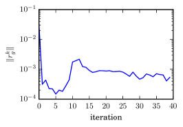
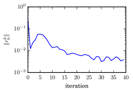
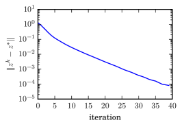
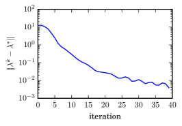
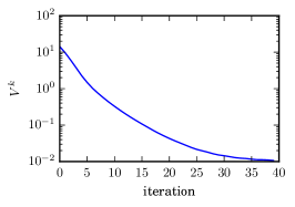
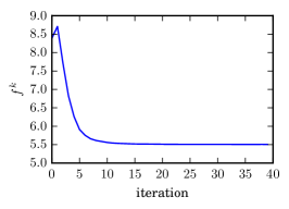
Figure 1: Various statistics for the performance of the distributed ADMM extension on an instance of the robust SVM problem. The convergence proof only states that the value $V^{k}$ must be monotonically decreasing. This can be observed also experimentally in the figure on the bottom right. Neither the primal function value nor the residuals need to be monotonically decreasing, and as can be seen in the figures on the top, they actually do not decrease monotonically.

Figure 1 shows the primal objective function value $f^{k}$, the norm of the residuals $r_{g}^{k}$ and $r_{h}^{k}$, the distances $\|z^{k}-z^{*}\|$, $\|\lambda^{k}-\lambda^{*}\|$, and the value $V^{k}$ of one run of our algorithm for two compute nodes. Note, that only $V^{k}$ must be strictly monotonically decreasing according to our convergence analysis. The proof does not make any statement about the monotonicity of the other values, and as can be seen in Figure 1, such statements would actually not be true. All values decrease in the long run, but are not necessarily monotonically decreasing.

As can be seen in Figure 1 (top-left), the function value $f^{k}$ is actually increasing for the first few iterations, while the residuals $r_{g}^{k}$ for the inequality constraints become very small, see Figure 1 (top-middle). That is, within the first iterations each compute node finds a solution to its share of the data that is almost feasible but has a higher function value than the true optimal solution. This basically means that the errors $\xi_{i}$ for the data points are over-estimated. After a few more iterations the primal function value drops and the inequality residuals increase meaning that the error terms $\xi_{i}$ as well as the individual estimators $w_{i}$ converge to their optimal values.

In the long run, the local estimators at the different compute nodes converge to the same solution. This is witnessed in Figure 1 (top-right), where one can see that the residuals $r_{h}^{k}$ for the consensus constraints converge to zero, i.e., consensus among the compute nodes is reached in the long run.

Finally, it can be seen that the consensus estimator $z^{k}$ converges to its unique optimal point $z^{*}$. Note that in general we cannot guarantee such a convergence since the optimal point does not need to be unique. But of course, in the special case that the optimal point is unique we always have convergence to this point.

7.4 Scalability results

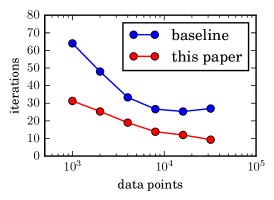
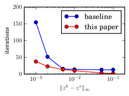
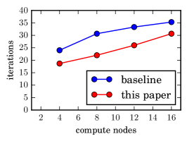
Figure 2: Running times of the algorithm on the robust SVM problem. The figure on the left shows that the number of iterations increases mildly with the number of compute nodes. The middle picture shows that the number of iterations is decreasing with increasing number of data points. The figure on the right shows the dependency of the distance of the consensus estimator $z^{k}$ in iteration $k$ to the optimal estimator $z^{*}$. It can be seen that our extension of ADMM outperforms the baseline approach with three nested loops.

Figure 2 shows the scalability of our extension of ADMM in terms of the number of compute nodes, data points, and approximation quality, respectively. All running times were measured in terms of iterations and averaged over runs for ten randomly generated data sets. The figures show the number of iterations for the approach presented in this paper and for the baseline, i.e., a three nested loops approach.

(1) For measuring the scalability in terms of employed compute nodes, we generated 10,000 data points with 10,000 features. As stopping criterion we used

$$\|z^{k}-z^{*}\|_{\infty}\leq 5\cdot 10^{-3},$$

i.e., the predictor $z^{k}$ had to be close to the optimum. Here we use the infinity norm to be independent from the number of dimensions. The data set was split into four, eight, twelve, and 16 equal sized batches that were distributed among the compute nodes. Note that every batch had much fewer data points than features, and thus the optimal solutions to the respective problems at the compute nodes were quite different from each other. Nevertheless, our algorithm converged very well to the globally optimal solution. Only the convergence speed was affected by the diversity of the local solutions at the different compute nodes. Since we kept the total number of data points in our experiments fixed, the diversity was increasing with the number of compute nodes that were assigned fewer data points each. Hence it was expected that the convergence speed decreases, i.e., the number of iterations increases, with a growing number of compute nodes. The expected behavior can be seen in Figure 2 (left). However, the increase is rather mild. The number of iterations less than doubles when the number of compute nodes increases from four to 16.

(2) For measuring the scalability in terms of the number of data points we increased the number of data points but kept the number of features fixed at 200. The stopping criterion for our algorithm was again

$$\|z^{k}-z^{*}\|_{\infty}\leq 5\cdot 10^{-3}.$$

We used eight compute nodes to compute the solutions. Again, the points were distributed equally among the compute nodes. This time one would expect a decreasing running time with an increasing number of data points, because the number of data points per machine is increasing and thus also the diversity of the local solutions at the different compute nodes is decreasing. That is, with an increasing number of data points it should take fewer iterations to reach an approximate consensus about the global solution among the compute nodes. The results of the experiment that are shown in Figure 2 (middle) confirm this expectation. The number of iterations indeed decreases with a growing number of data points. It has been noted before by Shalev-Shwartz and Srebro [22] that an increasing number of data points can require less work for providing a good predictor. We observe a similar phenomenon here.

(3) For measuring the scalability in terms of the approximation quality, we generated 8000 data points in 200 dimensions. Again, eight compute nodes were used for the experiments whose results are shown in Figure 2 (right). As expected the number of iterations (running time) increases with increasing approximation quality that was again measured in terms of the infinity norm. In this paper we are not providing a theoretical convergence rate analysis, which we leave for future work, but the experimental results shown here already provide some intuition on the dependency of the number of iterations in terms of the approximation quality: It seems that our extension of ADMM can solve problems to a medium accuracy within a reasonable number of iterations, but higher accuracy requires a significant increase in the number of iterations. Such a behavior is well known for standard ADMM without constraints [2]. In the context of our example application, robust SVMs, medium accuracy usually is sufficient as often higher accuracy solutions do not provide better predictors, a phenomenon that is also known as regularization by early stopping.

8 Conclusions

We have introduced and analyzed an algorithm for solving general convex optimization problems with many non-linear constraints in a distributed setting. The algorithm is based on an extension of the alternating direction method of multipliers (ADMM). Experiments on the robust SVM problem corroborate our theoretical convergence analysis and demonstrate the scalability of the approach in terms of the number of compute nodes as well as the number of data points.

Despite the vast literature on ADMM, to the best of our knowledge, an ADMM-like scheme for distributing general convex constraints has not been studied before. Standard ADMM is typically used for solving unconstrained optimization problems with separable objective function in a distributed fashion, but in principle standard ADMM can also be used for solving constrained optimization problems. This leads, in the distributed implementation of ADMM, to local, constrained optimization problems that have to be solved in every iteration. These local constrained optimization problems are easy to solve in special cases, for instance for linear constraints, but can become hard to solve in the general case of convex, non-linear constraints. In general three nested loops are necessary in this approach, an outer loop for reaching consensus, one loop for the constraints, and an inner loop for solving unconstrained problems. Alternatively, one can use the Augmented Lagrangian method for constrained optimization in the outer loop and standard ADMM in the inner loop. This approach also entails three nested loops, an outer loop for the constraints, one loop for reaching consensus, and an inner loop for solving unconstrained problems. That is, the tasks of the two outer loops, reaching consensus and dealing with the constraints, are interchanged in the two approaches. Here, we use the second approach, i.e., the Augmented Lagrangian with ADMM in the inner loop, as our baseline since it avoids the need for solving constrained problems in the inner loop. But our main contribution is showing that the two loops for reaching consensus and for handling constraints can be merged. This results in an extension of ADMM for dealing with problems with many, non-linear constraints in a distributed fashion that only needs two nested loops. To the best of our knowledge, we provide the first convergence proof for such a lazy algorithmic scheme. Experimental results provide evidence that our two-loop algorithm is indeed more efficient than the baseline approach with three nested loops.

Acknowledgments

This work was supported by Deutsche Forschungsgemeinschaft (DFG) under grant GI-711/5-1 and grant LA2971/1-1.

References

• [1] Martin Andersen, Joachim Dahl, Zhang Liu, and Lieven Vandenberghe. Interior-Point Methods for Large-Scale Cone Programming, pages 55–84. MIT Press, 2012.
• [2] Stephen P. Boyd, Neal Parikh, Eric Chu, Borja Peleato, and Jonathan Eckstein. Distributed optimization and statistical learning via the alternating direction method of multipliers. Foundations and Trends in Machine Learning, 3(1):1–122, 2011.
• [3] Tsung-Hui Chang, Mingyi Hong, and Xiangfeng Wang. Multi-agent distributed optimization via inexact consensus admm. IEEE Transactions on Signal Processing, 63(2):482–497, 2015.
• [4] Caihua Chen, Bingsheng He, Yinyu Ye, and Xiaoming Yuan. The direct extension of admm for multi-block convex minimization problems is not necessarily convergent. Mathematical Programming, 155(1-2):57–79, 2016.
• [5] Liang Chen, Defeng Sun, and Kim-Chuan Toh. An efficient inexact symmetric gauss–seidel based majorized admm for high-dimensional convex composite conic programming. Mathematical Programming, 161(1-2):237–270, 2017.
• [6] Wei Deng and Wotao Yin. On the global and linear convergence of the generalized alternating direction method of multipliers. Journal of Scientific Computing, 66(3):889–916, 2016.
• [7] Daniel Gabay and Bertrand Mercier. A dual algorithm for the solution of nonlinear variational problems via finite element approximation. Computers & Mathematics with Applications, 2(1):17 – 40, 1976.
• [8] Euhanna Ghadimi, André Teixeira, Iman Shames, and Mikael Johansson. Optimal parameter selection for the alternating direction method of multipliers (admm): Quadratic problems. IEEE Trans. Automat. Contr., 60(3):644–658, 2015.
• [9] R. Glowinski and A. Marroco. Sur l’approximation, par éléments finis d’ordre un, et la résolution, par pénalisation-dualité d’une classe de problèmes de dirichlet non linéaires. ESAIM: Mathematical Modelling and Numerical Analysis - Modélisation Mathématique et Analyse Numérique, 9(R2):41–76, 1975.
• [10] Bingsheng He and Xiaoming Yuan. On the O(1/n) convergence rate of the douglas–rachford alternating direction method. SIAM Journal on Numerical Analysis, 50(2):700–709, 2012.
• [11] Bingsheng He and Xiaoming Yuan. On non-ergodic convergence rate of douglas–rachford alternating direction method of multipliers. Numerische Mathematik, 130(3):567–577, 2015.
• [12] Magnus R. Hestenes. Multiplier and gradient methods. Journal of Optimization Theory and Applications, 4(5):303–320, 1969.
• [13] Mingyi Hong and Zhi-Quan Luo. On the linear convergence of the alternating direction method of multipliers. Mathematical Programming, pages 1–35, 2012.
• [14] Kejun Huang and Nicholas D Sidiropoulos. Consensus-admm for general quadratically constrained quadratic programming. IEEE Transactions on Signal Processing, 64(20):5297–5310, 2016.
• [15] Tianyi Lin, Shiqian Ma, and Shuzhong Zhang. On the global linear convergence of the admm with multiblock variables. SIAM Journal on Optimization, 25(3):1478–1497, 2015.
• [16] Zhouchen Lin, Risheng Liu, and Zhixun Su. Linearized alternating direction method with adaptive penalty for low-rank representation. In Advances in Neural Information Processing Systems (NIPS), pages 612–620, 2011.
• [17] José Luis Morales and Jorge Nocedal. Remark on ”algorithm 778: L-BFGS-B: fortran subroutines for large-scale bound constrained optimization”. ACM Trans. Math. Softw., 38(1):7:1–7:4, 2011.
• [18] Damon Mosk-Aoyama, Tim Roughgarden, and Devavrat Shah. Fully distributed algorithms for convex optimization problems. SIAM Journal on Optimization, 20(6):3260–3279, 2010.
• [19] Robert Nishihara, Laurent Lessard, Benjamin Recht, Andrew Packard, and Michael I Jordan. A general analysis of the convergence of admm. In International Conference on Machine Learning (ICML), pages 343–352, 2015.
• [20] M. J. D. Powell. Algorithms for nonlinear constraints that use lagrangian functions. Mathematical Programming, 14(1):224–248, 1969.
• [21] Katya Scheinberg, Shiqian Ma, and Donald Goldfarb. Sparse inverse covariance selection via alternating linearization methods. In Advances in Neural Information Processing Systems (NIPS), pages 2101–2109, 2010.
• [22] Shai Shalev-Shwartz and Nathan Srebro. SVM optimization: inverse dependence on training set size. In International Conference on Machine Learning (ICML), pages 928–935, 2008.
• [23] Pannagadatta K. Shivaswamy, Chiranjib Bhattacharyya, and Alexander J. Smola. Second order cone programming approaches for handling missing and uncertain data. Journal of Machine Learning Research, 7:1283–1314, 2006.
• [24] Morton Slater. Lagrange multipliers revisited. Cowles Foundation Discussion Papers 80, Cowles Foundation for Research in Economics, Yale University, 1950.
• [25] Ivor W. Tsang, András Kocsor, and James T. Kwok. Simpler core vector machines with enclosing balls. In International Conference on Machine Learning (ICML), pages 911–918, 2007.
• [26] E. Alper Yildirim. Two algorithms for the minimum enclosing ball problem. SIAM Journal on Optimization, 19(3):1368–1391, 2008.
• [27] Ruiliang Zhang and James T Kwok. Asynchronous distributed admm for consensus optimization. In International Conference on Machine Learning (ICML), pages 1701–1709, 2014.
• [28] Ciyou Zhu, Richard H. Byrd, Peihuang Lu, and Jorge Nocedal. Algorithm 778: L-BFGS-B: fortran subroutines for large-scale bound-constrained optimization. ACM Trans. Math. Softw., 23(4):550–560, 1997.
• [29] Minghui Zhu and Sonia Martínez. On distributed convex optimization under inequality and equality constraints. IEEE Trans. Automat. Contr., 57(1):151–164, 2012.