Low-Rank Dynamic Mode Decomposition:

Abstract

This work studies the linear approximation of high-dimensional dynamical systems using low-rank dynamic mode decomposition (DMD). Searching this approximation in a data-driven approach is formalized as attempting to solve a low-rank constrained optimization problem. This problem is non-convex and state-of-the-art algorithms are all sub-optimal. This paper shows that there exists a closed-form solution, which is computed in polynomial time, and characterizes the $\ell_{2}$-norm of the optimal approximation error. The paper also proposes low-complexity algorithms building reduced models from this optimal solution, based on singular value decomposition or eigen value decomposition. The algorithms are evaluated by numerical simulations using synthetic and physical data benchmarks.

1 Introduction

1.1 Context

The numerical discretization of a partial differential equation parametrized by its initial condition often leads to a very high dimensional system of the form:

$$\left\{\begin{aligned} &x_{t}(\theta)=f_{t}(x_{t-1}(\theta))\\ &x_{1}(\theta)={\theta}\end{aligned}\right.,\quad t=2,\ldots,T,\vspace{-0.cm}$$ (1)

where $x_{t}(\theta)\in\mathds{R}^{n}$ is the state variable, $f_{t}:\mathds{R}^{n}\to\mathds{R}^{n}$, and $\theta\in\mathds{R}^{n}$ denotes an initial condition. In some context, e.g., for uncertainty quantification purposes, one is interested by computing a set of trajectories corresponding to different initial conditions $\theta\in\Theta\subset\mathds{R}^{n}$. This may constitute an intractable task due to the high dimensionality of the space embedding the trajectories. For instance, in the case where $f_{t}$ is linear, the complexity required to compute a trajectory of model (1) scales in $\mathcal{O}(Tn^{2})$, which is prohibitive for large values of $n$ or $T$.

To deal with these large values, reduced models approximate the trajectories of the system for a range of regimes determined by a set of initial conditions 2015arXiv150206797C . A common assumption is that the trajectories of interest are well approximated in a low-dimensional subspace of $\mathds{R}^{n}$. In this spirit, many tractable approximations of model (1) have been proposed, in particular the well-known Petrov-Galerkin projection quarteroni2015reduced . However, these methods require the knowledge of the equations ruling the high-dimensional system.

Alternatively, there exist data-driven approaches. In particular, linear inverse modeling penland1993prediction , principal oscillating patterns Hasselmann88 , or more recently, dynamic mode decomposition (DMD) Chen12 ; 2016Dawson ; hemati2017biasing ; Jovanovic12 ; kutz2016dynamic ; Schmid10 ; Tu2014391 propose to approximate the unknown function $f_{t}$ by a linear and low-rank operator. This linear framework has been extended to quadratic approximations of $f_{t}$ in CuiMarzoukWillcox2014 . Although linear approximations are in appearance restrictive, they have recently sparked a new surge of interest because they are at the core of the so-called extended DMD or kernel-based DMD budivsic2012applied ; li2017extended ; williams2015data ; williams2014kernel ; 2017arXiv170806850Y . The latter decompositions characterize accurately non-linear behaviours under certain conditions klus2015numerical .

Reduced models based on low-rank linear approximations substitute function $f_{t}$ by a matrix $\hat{A}_{k}\in\mathds{R}^{n\times n}$ with $r={\textrm{rank}(\hat{A}_{k})}\leq n$ as

$$\left\{\begin{aligned} &\tilde{x}_{t}(\theta)=\hat{A}_{k}\tilde{x}_{t-1}(\theta),\quad t=2,\ldots,T,\\ &\tilde{x}_{1}(\theta)={\theta},\end{aligned}\right.\vspace{-0.cm}$$ (2)

where $\{\tilde{x}_{t}(\theta)\}_{t=1}^{T}$ denotes an approximation of the trajectory $\{x_{t}(\theta)\}_{t=1}^{T}$ of system (1). The complexity for the evaluation of a trajectory approximation with (2) will be refered to as on-line complexity. A low on-line complexity is obtained by exploiting the low rank of matrix $\hat{A}_{k}$. A scaling in $\mathcal{O}(Tr^{2}+rn)$ is reached if the reduced model is parametrized by matrices $R,\,L\in\mathds{C}^{n\times r}$ and $S\in\mathds{C}^{r\times r}$ such that trajectories of (2) correspond to the recursion

$$\left\{\begin{aligned} &\tilde{x}_{t}(\theta)=Rz_{t},\quad t=2,\ldots,T,\\ &z_{t}=Sz_{t-1},\,\,\,\quad t=3,\ldots,T,\\ &z_{2}=L^{\intercal}\theta.\end{aligned}\right.$$ (3)

The equivalence of systems (2) and (3) is obtained for $T\geq 2$ by setting $\hat{A}_{k}^{T-1}=RS^{T-2}L^{\intercal}$. In particular, consider a factorization of the form

$$\hat{A}_{k}=PQ^{\intercal}\quad\textrm{with}\quad P,Q\in\mathds{R}^{n\times r}.$$ (4)

This factorization is always possible by computing the singular value decomposition (SVD) ${\hat{A}_{k}}=U_{\hat{A}_{k}}\Sigma_{\hat{A}_{k}}V_{\hat{A}_{k}}^{\intercal}$ and identifying $P=U_{\hat{A}_{k}}$ and $Q^{\intercal}=\Sigma_{\hat{A}_{k}}V_{\hat{A}_{k}}^{\intercal}$. Factorization (4) implies that trajectories of (2) are obtained with system (3) setting $R=P$, $L=Q$ and $S=Q^{\intercal}P$. Another factorization of interest relies on the eigenvalue decomposition (EVD)

$$\hat{A}_{k}=D\Lambda D^{-1},\quad\textrm{with}\quad D,\Lambda\in\mathds{C}^{n\times n},$$ (5)

where $\Lambda$ is a Jordan-block matrix golub2013matrix of rank $r.$ Using the “economy size” EVD yields a system of the form of (3). Indeed, it is obtained by making the identification $L=(\xi_{1}\cdots\xi_{r})$ and $R=(\zeta_{1}\cdots\zeta_{r})$, where $\xi_{i}\in\mathds{C}^{n}$ and $\zeta_{i}\in\mathds{C}^{n}$ are the $i$-th left and right eigenvectors of $\hat{A}_{k}$ (equivalently the $i$-th column of $(D^{-1})^{\intercal}$ and $D$), and identifying $S$ to the first $r\times r$ block of $\Lambda$ multiplied by $L^{\intercal}$.

The on-line complexity to compute this recursion is still $\mathcal{O}(Tr^{2}+rn)$. But assuming that $\hat{A}_{k}$ is diagonalizable, we have $S=\textrm{diag}(\lambda_{1},\cdots,\lambda_{r})$ and system (3) becomes

$$\left\{\begin{aligned} \tilde{x}_{t}(\theta)&=\sum_{i=1}^{r}\zeta_{i}\nu_{i,t},\\ \nu_{i,t}&=\lambda_{i}^{t-1}\xi_{i}^{\intercal}\theta,\quad\textrm{for}\quad i=1,\ldots,\textrm{rank}(\hat{A}_{k})\end{aligned}\right.,\quad t=2,\ldots,T,\vspace{-0.cm}$$ (6)

where $\lambda_{i}\in\mathds{C}$ is the $i$-th (non-zero) eigenvalue of $\hat{A}_{k}$. This reduced-model possesses a very desirable on-line complexity of $\mathcal{O}(rn)$, i.e., linear in the ambient dimension $n$, linear in the reduced-model intrinsic dimension $r$ and independent of the trajectory length $T$.

The key of reduced modeling is to find a “good” tradeoff between the on-line complexity and the accuracy of the approximation. As shown previously, the low on-line computational effort is obtained by a proper factorization of the low-rank matrix $\hat{A}_{k}$. Thus, in an off-line stage, it remains to i) search $\hat{A}_{k}$ within the family of low-rank matrices which yields the “best” approximation (2), ii) compute the SVD or EVD based factorization of $\hat{A}_{k}$. We will refer to the computational cost associated to these two steps as off-line complexity.

A standard choice is to select $\hat{A}_{k}$ inducing the best trajectory approximation in the $\ell_{2}$-norm sense, for initial conditions in the set $\Theta\subset\mathds{R}^{n}$: matrix $\hat{A}_{k}$ in (2) targets the solution of the following minimization problem for some given $k\leq n$:

$$\operatorname*{arg\,min}_{A:\textrm{rank}(A)\leq k}\int_{\theta\in\Theta}\sum_{t=2}^{T}\|x_{t}(\theta)-A^{t-1}\theta\|^{2}_{2},$$ (7)

where $\|\cdot\|_{2}$ denotes the $\ell_{2}$-norm. Since we focus on data-driven approaches, we assume that we do not know the exact form of $f_{t}$ in (1) and we only have access to a set of representative trajectories $\{x_{t}(\theta_{i})\}_{t=1}^{T}$, $i=1,...,N$ so-called snapshots, obtained by running the high-dimensional system for $N$ different initial conditions $\{\theta_{i}\}_{i=1}^{N}$ in the set $\Theta$. Using these snapshots, we consider a discretized version of (7), which corresponds to the constrained optimization problem studied in Chen12 ; Jovanovic12 ; wynn2013optimal : matrix $\hat{A}_{k}$ now targets the solution

$$A_{k}^{\star}\in \operatorname*{arg\,min}_{A:\textrm{rank}(A)\leq k}\sum_{i=1}^{N}\sum_{t=2}^{T}\|x_{t}(\theta_{i})-Ax_{t-1}(\theta_{i})\|^{2}_{2},$$ (8)

where we have substituted $A^{t-1}\theta_{i}$ in (7) by $Ax_{t-1}(\theta_{i})$ and where we have approximated the integral by an empirical average over the snapshots.

Problem (8) is non-convex due to the presence of the rank constraint “$\textrm{rank}(A)\leq k$”. As consequence, it has been considered as intractable in several contributions of the litterature and numerous procedures have been proposed to approximate its solution (see next section). In this paper, we show that problem (8) is in fact tractable and admits a closed-form solution which can be evaluated in polynomial-time.

1.2 Problem Statement and Contributions

This work deals with the off-line construction of reduced models of the form of (3). It focuses on the following questions:

1. Can we compute a solution of problem (8) in polynomial time?

2. How to compute efficiently a factorization of this solution, and in particular its EVD?

Let us make some correspondences with the terminology used in the DMD literature Chen12 ; 2016Dawson ; hemati2017biasing ; Jovanovic12 ; kutz2016dynamic ; Schmid10 ; Tu2014391 in order to reformulate these two questions in the jargon used in this community. The “low-rank DMD” of system (1) refers to the EVD of the solution $A_{k}^{\star}$ of problem (8), or equivalently to the parameters of reduced model (6) in the case where $\hat{A}_{k}=A_{k}^{\star}$ is diagonalizable. Using this terminology, the two above questions can be summarized summarized as follows: can we compute exactly and with a polynomial complexity the low-rank DMD of system (1)? In this paper, we show that the answer to this question is positive and provide some numerical procedures to attain this goal.

Solver for problem (8).  In the last decade, there has been a surge of interest for low-rank solutions of linear matrix equations, see e.g.,  fazel2002matrix ; jain2010guaranteed ; lee2009guaranteed ; lee2010admira ; mishra2013low ; recht2010guaranteed . This class of problems includes (8) as an important particular case. Problems in this class are always non-convex due to the rank constraint and computing their solutions in polynomial time is often out of reach. Nevertheless, certain instances of these problems with very special structures admit closed-form solutions eckart1936approximation ; mesbahi1997rank ; parrilo2000cone . In this work, we show that (8) belongs to this class of problems and provide a closed-form solution which can be computed in polynomial time. Prior to this work, many authors have proposed tractable procedures to compute approximations of the solution to problem (8)  Chen12 ; Jovanovic12 ; li2017extended ; Tu2014391 ; wynn2013optimal ; 2017arXiv170806850Y or to related problems hemati2017biasing . We review these contributions in Section 3.1 and discuss their complexity.

Factorization of the solution. The second problem concerns the computation of the factorization of the form (4) or (5) of the solution $A_{k}^{\star}\in\mathds{R}^{n\times n}$. A brute-force computation of a factorization of a matrix in $\mathds{R}^{n\times n}$, in particular an EVD, is prohibitive for large values of $n$. In this work, we propose low-complexity algorithms computing such factoization of $A_{k}^{\star}$. This follows the line and extends previous works Jovanovic12 ; Tu2014391 ; williams2014kernel , as detailed in Section 3.2.

In summary, the contribution of this paper is twofold. First, we provide a closed-form solution to (8). We also design an algorithm computing a factorized form of this solution with a linear complexity in the ambient dimension. Second, we provide an algorithm computing the EVD of this optimal solution, which does not imply an increase in complexity.

The paper is organized as follows. In Section 3, we provide a review of techniques approximating and factorizing the solution of problem (8). In Section 4, we present the proposed approach. Finally, in Section 5, we study the performance obtained with the proposed algorithms in synthetic and physical setups and compare with state-of-the-art.

2 Notations

All along the paper, we make extensive use of the economy-size SVD of a matrix $M\in\mathds{R}^{p\times q}$ with $p\geq q$: $M=U_{M}\Sigma_{M}V_{M}^{\intercal}$ with $U_{M}\in\mathds{R}^{p\times q}$, $V_{M}\in\mathds{R}^{q\times q}$ and $\Sigma_{M}\in\mathds{R}^{q\times q}$ so that $U_{M}^{\intercal}U_{M}=V_{M}^{\intercal}V_{M}=I_{q}$ and $\Sigma_{M}$ is diagonal, where the upper script $\cdot^{\intercal}$ refers to the transpose and $I_{q}$ denotes the $q$-dimensional identity matrix. The columns of matrices $U_{M}$ and $V_{M}$ are denoted $U_{M}=(u_{M}^{1}\cdots u_{M}^{q})$ and $V_{M}=(v_{M}^{1}\cdots v_{M}^{q})$ while $\Sigma_{M}=\textrm{diag}(\sigma_{M,1},\cdots,\sigma_{M,q})$ with $\sigma_{M,i}\geq\sigma_{M,i+1}$ for $i=1,\ldots,q-1$. The Moore-Penrose pseudo-inverse of matrix $M$ is then defined as $M^{\dagger}=V_{M}\Sigma^{\dagger}_{M}U_{M}^{\intercal}$, where $\Sigma^{\dagger}_{M}=\textrm{diag}(\sigma_{M,1}^{\dagger},\cdots,\sigma_{M,q}^{\dagger})$ with

$$\sigma_{M,i}^{\dagger}=\left\{\begin{aligned} &\sigma_{M,i}^{-1}\quad\textrm{if}\quad\sigma_{M,i}>0\\ &0\quad\quad\,\,\,\textrm{otherwise}\end{aligned}\right..\vspace{-0.cm}\\$$

The orthogonal projector onto the span of the columns (resp. of the rows) of matrix $M$ is denoted by $\mathbb{P}_{M}=MM^{\dagger}=U_{M}\Sigma_{M}\Sigma_{M}^{\dagger}U_{M}^{\intercal}$ (resp. $\mathbb{P}_{M^{\intercal}}=M^{\dagger}M=V_{M}\Sigma_{M}^{\dagger}\Sigma_{M}V_{M}^{\intercal}$) golub2013matrix .

We also introduce additional notations to derive a matrix formulation of the low-rank estimation problem (8). We gather consecutive elements of the $i$-th snapshot trajectory between time $t_{1}$ and $t_{2}$ in matrix $X_{t_{1}:t_{2}}^{(i)}~{}=~{}(x_{t_{1}}(\theta_{i})\cdots x_{t_{2}}(\theta_{i}))$ and form large matrices $\mathbf{X},\mathbf{Y}\in\mathds{R}^{n\times m}$ with $m=N(T-1)$ as

$$\mathbf{X}=(X^{(1)}_{1:T-1}\cdots X^{(N)}_{1:T-1})\quad\textrm{and}\quad\mathbf{Y}=(X^{(1)}_{2:T}\cdots X^{(N)}_{2:T}).$$

In order to be consistent with the SVD definition and to keep the presentation as simple as possible, this work assumes that $m\leq n$. However, all the result presented in this work can be extended without any difficulty to the case where $m>n$ by using an alternative definition of the SVD.

3 State-Of-The-Art Approximations

We begin by presenting state-of-the-art methods solving approximatively the low-rank minimization problem (8). In a second part, we make an overview of state-of-the-art algorithms computing factorizations of these approximated solutions of the form of (4) or (5).

3.1 Tractable Approximations to Problem (8)

Using the notations introduced in Section 2, problem (8) can be rewritten as

$$A_{k}^{\star}\in \operatorname*{arg\,min}_{A:\mathrm{rank}(A)\leq k}\|{\mathbf{Y}}-A{\mathbf{X}}\|^{2}_{F},$$ (9)

where $\|\cdot\|_{F}$ refers to the Frobenius norm. A detailed review of the following state-of-the-art approximations of $A_{k}^{\star}$ is provided in our technical note HeasHerzet17 .

Truncation of the unconstrained solution. A first approximation consists in removing the low-rank constraint in problem (9). As pointed out by Tu et al. in Tu2014391 , the problem then boils down to a least-squares problem

$$\operatorname*{arg\,min}_{A}\|{\mathbf{Y}}-A{\mathbf{X}}\|^{2}_{F},$$ (10)

admitting the closed-form solution ${\mathbf{Y}}{\mathbf{X}}^{\dagger}$. Matrix ${\mathbf{Y}}{\mathbf{X}}^{\dagger}$ also solves the constrained problem (9) in the case where $k\geq m$ and in particular for $k=m$, i.e.,

$$A^{\star}_{m}={\mathbf{Y}}{\mathbf{X}}^{\dagger}.$$ (11)

This solution relies on the SVD of $\mathbf{X}$: $A^{\star}_{m}={\mathbf{Y}}V_{{\mathbf{X}}}\Sigma_{{\mathbf{X}}}^{\dagger}U_{{\mathbf{X}}}^{\intercal},$ which is computed with a complexity of $\mathcal{O}(m^{2}(m+n))$ golub2013matrix . An approximation of the solution of (9) satisfying the low-rank constraint $\textrm{rank}(A)\leq k$ with $k<m$ is then obtained by a truncation of the SVD or the EVD of $A^{\star}_{m}$ using $k$ terms.

Approximation by low-rank projected DMD. The “projected DMD” proposed by Schmid Schmid10 is an approximation of $A^{\star}_{m}$, which assumes that the columns of $A^{\star}_{m}{\mathbf{X}}$ are in the span of ${\mathbf{X}}$. This assumption is used by Jovanovic et al. Jovanovic12 to approximate $A^{\star}_{k}$ for $k<m$. Their approach yields the so-called “low-rank projected DMD” approximation of (9) which takes the following form

$$A_{k}^{\star}\approx U_{{\mathbf{X}}}\tilde{Y}_{k}\Sigma_{{\mathbf{X}}}^{\dagger}U_{{\mathbf{X}}}^{\intercal},$$ (12)

where $\tilde{Y}_{k}$ denotes the SVD representation of matrix $\tilde{Y}=U_{{\mathbf{X}}}^{\intercal}{\mathbf{Y}}V_{{\mathbf{X}}}$ truncated to $k$ terms. Similar low-dimensional parametrizations of the optimal solution $A_{k}^{\star}$ are used to compute the so-called “optimized DMD” in Chen12 or “optimal mode decomposition” in wynn2013optimal . The computation of low-rank projected DMD relies on the SVD of ${\mathbf{X}}\in\mathds{R}^{n\times m}$ and $\tilde{Y}\in\mathds{R}^{m\times m}$ and thus involves a complexity of $\mathcal{O}(m^{2}(m+n))$ golub2013matrix .

Approximation by sparse DMD. Jovanovic et al. also propose in Jovanovic12 a two-stage approach which consists in searching a $k$ terms approximation of the EVD of an unconstrained projected DMD, i.e., the EVD of $U_{{\mathbf{X}}}\tilde{Y}\Sigma_{{\mathbf{X}}}^{\dagger}U_{{\mathbf{X}}}^{\intercal}$. The optimal truncated EVD is efficiently computed solving a relaxed convex optimization problem taking advantage of the EVD of $\tilde{Y}\Sigma_{{\mathbf{X}}}^{\dagger}\in\mathds{R}^{m\times m}$. The overall complexity of this procedure scales as $\mathcal{O}(m^{2}(m+n))$.

Approximation by total-least-square DMD. This approximation is proposed by Hemati et al. hemati2017biasing . Using the projector $\mathbb{P}_{\mathbf{K}^{\intercal},k}={V}_{\mathbf{K},k}({V}_{\mathbf{K},k})^{\intercal}$ where the columns of ${V}_{\mathbf{K},k}\in\mathbb{R}^{m\times k}$ are the right singular vectors associated to the $k$ largest singular values of matrix $\mathbf{K}=\begin{bmatrix}{\mathbf{X}}^{\intercal}&{\mathbf{Y}}^{\intercal}\end{bmatrix}^{\intercal}\in\mathds{R}^{2n\times m}$, the total-least-square DMD (TLS DMD) approximation takes the form of

$$A_{k}^{\star}\approx{\mathbf{Y}}\mathbb{P}_{\mathbf{K}^{\intercal},k}{\mathbf{X}}^{\dagger}.$$ (13)

This method relies on the SVD of $\mathbf{K}\in\mathds{R}^{2n\times m}$ and $\mathbf{X}\in\mathds{R}^{n\times m}$ and has thus a complexity of $\mathcal{O}(m^{2}(m+n))$.

Approximation by convex relaxation. Some works propose to approximate (9) by a regularized version of the unconstrained problem (10), using Tikhonov penalization li2017extended or penalization enforcing structured sparsity 2017arXiv170806850Y . However, these choices of regularizers do not guarantee in general that the solution is low-rank. In contrast, the solution of (9) may under certain theoretical conditions lee2010admira ; jain2010guaranteed be recovered by the following quadratic program

$$A_{k}^{\star} \approx\operatorname*{arg\,min}_{A\in\mathds{R}^{n\times n}}\|{\mathbf{Y}}-A{\mathbf{X}}\|^{2}_{F}+\alpha_{k}\|A\|_{*},$$

$$=\operatorname*{arg\,min}_{A\in\mathds{R}^{n\times n}}\min_{B\in\mathds{R}^{n\times n}}\|{\mathbf{Y}}-A{\mathbf{X}}\|^{2}_{F}+\alpha_{k}\|B\|_{*}\quad\textrm{s.t.}\quad A=B$$ (14)

where $\|\cdot\|_{*}$ refers to the nuclear norm (or trace norm) of the matrix, i.e., the sum of its singular values. In optimization problem (3.1), $\alpha_{k}\in\mathds{R}_{+}$ represents an appropriate regularization parameter determining the rank $k$ of the solution. Program (3.1) is a convex optimization problem mishra2013low which can be efficiently solved using modern optimization techniques, such as the alternate directions of multipliers method (ADMM) bertsekas1995nonlinear . The algorithms solving (3.1) typically involve per iteration a complexity of $\mathcal{O}(m(m^{2}+n^{2}))$.

3.2 Factorizations of Approximations of $A_{k}^{\star}$

In this section, we provide an overview of some state-of-the-art methods to compute factorizations of the form of (4) or (5) for the approximations of $A_{k}^{\star}$ presented above.

We first note that a brute-force computation of the SVD or EVD of a matrix in $\mathds{R}^{n\times n}$ leads in general to a prohibitive computational cost since it requires a complexity of $\mathcal{O}(n^{3})$. Hopefully, the factorizations (4) or (5) are computable with a complexity of $\mathcal{O}(m^{2}(m+n))$, in most cases mentioned above.

In particular, in the case of low-rank projected DMD, a straightforward factorization of the form of (4) is $P=U_{\mathbf{X}}$ and $Q^{\intercal}=\tilde{Y}_{k}\Sigma_{{\mathbf{X}}}^{\dagger}U_{{\mathbf{X}}}^{\intercal}$. In the case of sparse DMD, the latter factorization holds by substituting $\tilde{Y}_{k}$ by the “sparse” approximation of $\tilde{Y}$. Another straightforward factorization of the form of (4) is intrinsic to the ADMM procedure, which uses an SVD to compute the regularized solution.

Concerning EVD factorization, in the case of the truncated approach, Tu et al. propose an algorithm scaling in $\mathcal{O}(m^{2}(m+n))$ Tu2014391 . In the context of low-rank projected DMD or sparse DMD, Jovanovic et al. propose a procedure of analogous complexity, which approximates the first $m$ eigenvectors, and then estimate the related eigenvalues by solving a convex optimization problem Jovanovic12 . In the case of TLS DMD, the diagonalization of a certain matrix in $\mathds{R}^{m\times m}$ suffices to obtain the sought EVD factorization.

In summary, on the one hand, we saw in Section 3.1 that all existing algorithms compute in general sub-optimal solutions of problem (9). On the other hand, the literature does not provide a “turnkey” algorithm for factorizing the optimal solution $A^{\star}_{k}$ in the form of (4) or (5), with a reduced complexity of $\mathcal{O}(m^{2}(m+n))$. In the next section, we show how to compute an optimal solution $A^{\star}_{k}$ and compute efficiently its factorization.

4 The Proposed Approach

In this section, we provide a closed-form solution to problem (9). Algorithms are then proposed to compute and factorize this solution in the form of (4) or (5).

4.1 Closed-Form Solution to (9)

Let the columns of matrix ${U}_{\mathbf{Z},k}=\begin{pmatrix}u^{1}_{\mathbf{Z}}&\cdots&u^{k}_{\mathbf{Z}}\end{pmatrix}\in\mathds{R}^{n\times k}$ be the left singular vectors $\{u_{\mathbf{Z}}^{i}\}_{i=1}^{k}$ associated to the $k$ largest singular values of matrix

$$\mathbf{Z}={\mathbf{Y}}\mathbb{P}_{{\mathbf{X}}^{\intercal}}\in\mathds{R}^{n\times m},$$ (15)

where we recall that $\mathbb{P}_{{\mathbf{X}}^{\intercal}}={V}_{\mathbf{X}}{V}_{\mathbf{X}}^{\intercal}$ and consider the projector

$$\mathbb{P}_{\mathbf{Z},k}={U}_{\mathbf{Z},k}{{U}_{\mathbf{Z},k}}^{\intercal}.$$ (16)

Matrix (16) appears in the closed-form solution of (9), as shown in the following theorem. We detail the proof in Appendix A.

Theorem 4.1

Problem (9) admits the following solution

$$A_{k}^{\star}=\mathbb{P}_{\mathbf{Z},k}{\mathbf{Y}}{\mathbf{X}}^{\dagger}.$$ (17)

Moreover, the optimal approximation error can be expressed as

$$\|{\mathbf{Y}}-A_{k}^{\star}{\mathbf{X}}\|^{2}_{F}=\sum_{i=k+1}^{m}\sigma_{\mathbf{Z},i}^{2}+\|{\mathbf{Y}}(I_{m}-\mathbb{P}_{{\mathbf{X}}^{\intercal}})\|_{F}^{2}.$$ (18)

In words, Theorem 4.1 shows that problem (9) is simply solved by computing the orthogonal projection of the solution of the unconstrained problem (10), onto the subspace spanned by the first $k$ left singular vectors of $\mathbf{Z}.$ The $\ell_{2}$-norm of the error is simply expressed in terms of the singular values of $\mathbf{Z}$, and the square norm of the projection of the rows of ${\mathbf{Y}}$ onto the orthogonal of the image of ${\mathbf{X}}^{\intercal}$. If ${\mathbf{X}}$ is full row-rank, we then obtain the simplifications $\mathbb{P}_{{\mathbf{X}}^{\intercal}}=I_{m}$ and $\mathbf{Z}={\mathbf{Y}}$. In this case, the second term in the right-hand side of (18) vanishes and the approximation error reduces to $\|{\mathbf{Y}}-A_{k}^{\star}{\mathbf{X}}\|^{2}_{F}=\sum_{i=k+1}^{m}\sigma_{{\mathbf{Y}},i}^{2}$. The latter error is independent of matrix ${\mathbf{X}}$ and is simply the sum of the square of the $m-k$ smallest singular values of ${\mathbf{Y}}$. This error also corresponds to the optimal error for the approximation ${\mathbf{Y}}$ by a matrix of rank at most $k$ in the Frobenius norm eckart1936approximation .

It is worth mentioning that we propose in HeasHerzet18Maps a generalization of Theorem 4.1 to separable infinite-dimensional Hilbert spaces. This generalization characterizes the solution of low-rank approximations in reproducing kernel Hilbert spaces (where $n=\infty$) at the core of kernel-based DMD HeasIcassp2020 ; williams2014kernel , and characterizes the solution of the DMD counterpart (where $m=\infty$) to the continuous POD problem presented in (quarteroni2015reduced, , Theorem 6.2).

4.2 Algorithm Evaluating $A_{k}^{\star}$

inputs: $(\mathbf{X},\mathbf{Y}).$

1) Compute the SVD of ${\mathbf{X}}=V_{{\mathbf{X}}}\Sigma^{\dagger}_{{\mathbf{X}}}U_{{\mathbf{X}}}^{\intercal}$

2) Compute $\mathbf{Z}={\mathbf{Y}}V_{{\mathbf{X}}}\Sigma_{{\mathbf{X}}}\Sigma_{{\mathbf{X}}}^{\dagger}V_{{\mathbf{X}}}^{\intercal}$.

3) Compute the SVD of $\mathbf{Z}$ to obtain the projector $\mathbb{P}_{\mathbf{Z},k}$.

4) Compute $A_{k}^{\star}=\mathbb{P}_{\mathbf{Z},k}{\mathbf{Y}}V_{{\mathbf{X}}}\Sigma^{\dagger}_{{\mathbf{X}}}U_{{\mathbf{X}}}^{\intercal}$.

output: $A_{k}^{\star}$.

Algorithm 1 Computation of $A_{k}^{\star}$, a solution of (9)

The design of an algorithm computing the solution (17) is straightforward: evaluating $A_{k}^{\star}$ consists in making a product of easily-computable matrices. The proposed procedure is summarized in Algorithm 1.

Steps 1) to 3) of Algorithm 1 implies the computation of the SVD of matrices ${\mathbf{X}},\mathbf{Z}\in\mathds{R}^{n\times m}$, and matrix multiplications involving $m^{2}$ vector products in $\mathds{R}^{n}$ or $\mathds{R}^{m}$. The complexity of these first three steps is therefore $\mathcal{O}(m^{2}(m+n))$. Computing explicitly each entry of $A_{k}^{\star}\in\mathds{R}^{n\times n}$ in step 4) of Algorithm 1 then requires a complexity of $\mathcal{O}(n^{2}k)$, which is prohibitive for large $n$. However, as detailed in the next section, this last step is not necessary to factorize the optimal solution $A^{\star}_{k}$ in the form of (4) or (5).

4.3 Algorithms Factorizing $A_{k}^{\star}$

Given the closed-form solution (17), we present in what follows how to compute from ${\mathbf{X}}$ and ${\mathbf{Y}}$ a factorization of the optimal solution $A^{\star}_{k}$ in the form of (4) or (5). We will need matrix

$${W}=({{U}_{\mathbf{Z},k}}^{\intercal}{\mathbf{Y}}{\mathbf{X}}^{\dagger})^{\intercal}\in\mathds{R}^{n\times k}.$$ (19)

Factorization of the form of (4). By performing the first three steps of Algorithm 1 and then making the identifications $P={U}_{\mathbf{Z},k}$ and $Q={W}$, we obtain a factorization of $A_{k}^{\star}$ of the form of (4). As mentioned in the introduction, trajectories of (2) can then be computed with system (3) setting $R={U}_{\mathbf{Z},k}$, $L=W$ and $S=W^{\intercal}{U}_{\mathbf{Z},k}$. The method relies on the first three steps of Algorithm 1 and on the computation of matrix ${W}$. The three steps in Algorithm 1 imply a complexity of $\mathcal{O}(m^{2}(m+n))$ while the computation of ${W}$ requires a complexity of $\mathcal{O}(nk^{2})$. Since $k\leq m$, the off-line complexity to build the factorization (4) from ${\mathbf{X}}$ and ${\mathbf{Y}}$ scales as $\mathcal{O}(m^{2}(m+n))$, which is the same order of complexity as the procedures described in Section 3.

inputs: $(\mathbf{X},\mathbf{Y}).$

1) Compute step 1 to 3 of Algorithm 1 and use (19) to obtain ${W}$.

2) Let $r=\textrm{rank}(A^{\star}_{k})$ and solve for $i=1,\ldots,r$ the eigen-equations

$$({W}^{\intercal}{U}_{\mathbf{Z},k})w^{r}_{i}=\lambda_{i}w^{r}_{i}\quad\textrm{and}\quad({{U}_{\mathbf{Z},k}}^{\intercal}{W})w^{\ell}_{i}=\lambda_{i}w^{\ell}_{i},$$

where $w^{r}_{i},w^{\ell}_{i}\in\mathds{C}^{k}$ and $\lambda_{i}\in\mathds{C}$ such that $|\lambda_{i+1}|\geq|\lambda_{i}|$.

3) Compute for $i=1,\ldots,r$ the right and left eigenvectors

$$\zeta_{i}={U}_{\mathbf{Z},k}w^{r}_{i}\quad\textrm{and}\quad{\xi_{i}}={W}w^{\ell}_{i}.$$ (20)

4) Rescale the ${\xi_{i}}$’s so that ${\xi_{i}}^{T}\zeta_{i}=1$.

outputs: $L=(\xi_{1}\cdots\xi_{r})$, $R=(\zeta_{1}\cdots\zeta_{r})$, $S=\textrm{diag}(\lambda_{1},\cdots,\lambda_{r}).$

Algorithm 2 EVD of $A^{\star}_{k}$ or low-rank DMD

Factorization of the form of (5). According to the previous factorization of the form of (4), $A^{\star}_{k}$ is the product of matrix ${U}_{\mathbf{Z},k}$ in $\mathds{R}^{n\times k}$ with matrix ${W}^{\intercal}$ in $\mathds{R}^{k\times n}$. Therefore, using standard matrix analysis, we expect the eigenvectors of $A^{\star}_{k}$ to belong to a $k$-dimensional subspace golub2013matrix . As shown in the next proposition, the non-zero eigenvalues of $A^{\star}_{k}$ are obtained by EVD of certain matrices in $\mathds{R}^{k\times k}$. The proof of this proposition is given in Appendix C.

Proposition 1

Assume $A^{\star}_{k}$ is diagonalizable. The elements of $\{\zeta_{i},\xi_{i},\lambda_{i}\}_{i=1}^{\mathrm{rank}(A^{\star}_{k})}$ generated by Algorithm 2 are the right eigenvectors, the left eigenvectors and the eigenvalues of the economy size EVD of $A^{\star}_{k}$.

In words, Proposition 1 shows that Algorithm 2 computes the EVD of $A^{\star}_{k}$ by diagonalizing two matrices in $\mathds{R}^{k\times k}$. The complexity to build this EVD from snapshots $\mathbf{X}$ and $\mathbf{Y}$ is $\mathcal{O}(m^{2}(m+n))$. More precisely, as mentioned previously, performing the first three steps of Algorithm 1 (i.e., step 1) of Algorithm 2) requires a number of operations scaling as $\mathcal{O}(m^{2}(m+n))$; the complexity of step 2) is $\mathcal{O}(k^{3})$ since it performs the EVDs of $k\times k$ matrices; step 3) involves $r\times n$ vector products in $\mathds{R}^{m}$ while step 4) involves $r$ vector products in $\mathds{R}^{n}$, with $r\leq k\leq m$. Overall, the complexity of Algorithm 2 is dominated by step 1) and the EVD of $A^{\star}_{k}$ can be evaluated with a computational cost of the order of $\mathcal{O}(m^{2}(m+n))$.

5 Numerical Evaluation

In what follows, we evaluate five different trajectory approximations $\tilde{x}_{t}(\theta)$ obtained by reduced model of the form of (6), obtained by EVD factorizations of different low-rank matrix approximations $\hat{A}_{k}$. The assessed low-rank matrix factorizations are listed below.

• Optimal approximation: the EVD of the optimal solution $A_{k}^{\star}$, provided by Algorithm 2.

• Approximation by truncated DMD Tu2014391 : the $k$-th order truncation of the EVD of the unconstrained problem solution $A^{\star}_{m}$ given in (11).

• Approximation by low-rank projected DMD Jovanovic12 : the EVD of the $k$-th order approximation (12).

• Approximation by TLS DMD hemati2017biasing : the EVD of (13).

• Approximation by convex relaxation: the EVD of the solution (3.1), the latter is computed by an ADMM procedure, where the regularization parameter $\alpha_{k}$ is adjusted to obtain a rank equal to $k$.

Rather than evaluating the error norm of the approximation, i.e., the cost of the target problem (7), we are interested in the ability of the different algorithms to minimize the cost of the proxy (9) for this problem. Therefore, the performance is measured in terms of the normalized reconstruction error norm ${\|{\mathbf{Y}}-\hat{A}_{k}{\mathbf{X}}\|_{F}}{\|{\mathbf{Y}}\|_{F}^{-1}}$ as a function of $k$. Besides, in the analysis perspective adopted most often in the DMD literature hemati2017biasing ; Jovanovic12 ; Schmid10 ; Tu2014391 , we are interested in evaluating the ability of the algorithms to compute accurately the EVD of $A^{\star}_{k}$. In particular, we quantify for a given $k$ the deviation of the set of the $k$ largest estimated eigenvalues $\lambda(\hat{A}_{k})\in\mathbb{C}^{k}$, from the non-zero optimal ones $\lambda(A^{\star}_{k})$ in terms of the normalized error norm ${\|\lambda(\hat{A}_{k})-\lambda(A^{\star}_{k})\|_{2}}{\|\lambda(A^{\star}_{k})\|_{2}^{-1}}$.

We begin by evaluating the performance of the low-rank approximations on a different toy models in Section 5.1. We then assess their performance for the reduction of a Rayleigh-Bénard convective system chandrasekhar2013hydrodynamic in Section 5.2. We finally evaluate the influence of noise on the estimation accuracy in Section 5.3.

5.1 Synthetic Experiments with Toy Models

Figure 1: Reconstruction error norm as a function of $k$ for setting $i)$, $ii)$ and $iii)$ (for $rank(\mathbf{X})=m$ and $rank(\mathbf{X})=m-6$) using our optimal approximation or state-of-the-art approximations. See details in Section 5.1.

Figure 2: Eigenvalue error norm as a function of $k$ for setting $i)$, $ii)$ and $iii)$ (for $\mathrm{rank}(\mathbf{X})=m$ and $\mathrm{rank}(\mathbf{X})=m-6$) using our optimal approximation or state-of-the-art approximations. See details in Section 5.1.

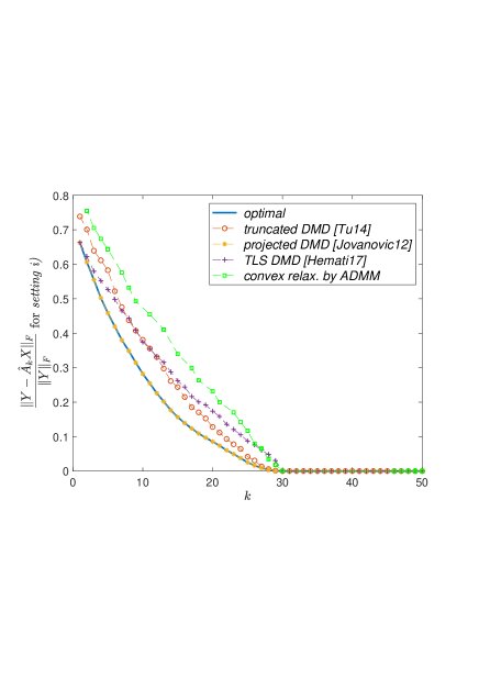
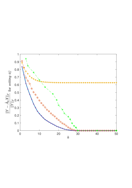
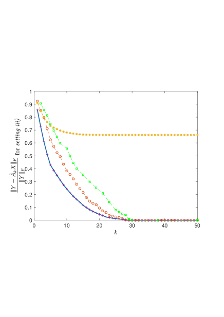
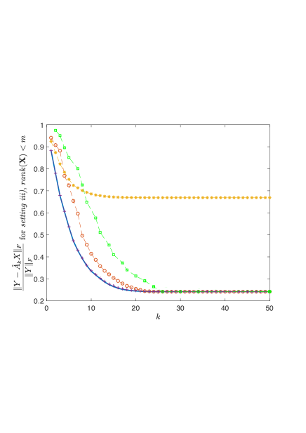
We set $n=50$, $N=30$ and set the trajectory length in (1) to $T=2$. Entries of matrices ${\mathbf{X}}$, i.e., the initial condition $\theta$, are such that ${\mathbf{X}}=\sum_{i=1}^{\textrm{rank}({\mathbf{X}})}\varphi_{i}\varphi_{i}^{\intercal}$ with $\textrm{rank}({\mathbf{X}})\leq m$ and where the $\varphi_{i}$’s are $n$-dimensional independent samples of the standard normal distribution. Matrix ${\mathbf{Y}}$ is then generated using model (1) and three different choices for $f_{t}$:

• setting i):   $f_{t}(x_{t-1})=Gx_{t-1}$, where $G$ is chosen such that $G{\mathbf{X}}\in\textrm{span}({\mathbf{X}})$,

• setting ii):   $f_{t}(x_{t-1})=Fx_{t-1}$,

• setting iii):   $f_{t}(x_{t-1})=F(x_{t-1}+x_{t-1}^{3})$.

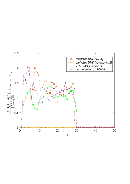
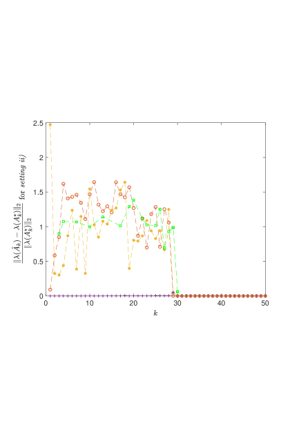
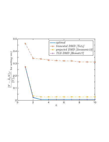
Matrix $F$ introduced above is a random matrices of rank $m$ defined as $F=\sum_{i=1}^{m}\varphi_{i}\varphi_{i}^{\intercal}$, where the $\varphi_{i}$’s represents a set of $n$-dimensional independent samples of the standard normal distribution. We define implicitly matrix $G$ of rank $m$ by drawing the parameters of the so-called companion matrix Schmid10 with independent samples of the standard normal distribution. The notation $x_{t-1}^{3}$ denotes that each entry of vector $x_{t-1}$ has been raised to the power $3$. The first setting is a linear system satisfying the sub-space assumption $G{\mathbf{X}}\in\textrm{span}({\mathbf{X}})$, on which low-rank projected DMD relies. The two next settings do not make this assumption and simulate respectively linear and cubic dynamics. The performance of the five methods in terms of reconstruction and eigenvalue errors are displayed in Figure 1 and 2.

In accordance with our theoretical results, the proposed algorithm yields the smallest error norms in all the scenarios. Moreover, in accordance with Theorem 4.1, as long as we have a full-rank matrix ${\mathbf{X}}$, the optimal solution reaches a zero reconstruction error for $k\geq m$ with $m=N(T-1)=30$ (we have considered $N=30$ snapshots and $T=2$ successive states). The deterioration of the reconstruction error norm for the approximation by truncated DMD shows that a two-stage approach is sub-optimal. However, this deterioration is moderate in these toy experiments. Moreover, the experiments show that the approximation by low-rank projected DMD achieves the optimal performance as long as the sub-space assumption holds, i.e., for setting i). If this assumption is not satisfied, i.e., in setting ii) and iii), we observe a poor performance of this projected approach for $k>10$. On the contrary to low-rank projected DMD, TLS DMD performs poorly in the case where $G{\mathbf{X}}\in\textrm{span}({\mathbf{X}})$, i.e., for setting i), while it yields a quasi-optimal error norm in the other settings. Furthermore, we observe that the approximation provided by a convex relaxation approach differs significantly from $A^{\star}_{k}$ in all the considered settings, as indicated by the error norm for $k<m$. This suggests that the theoretical conditions necessary to recover $A^{\star}_{k}$ by convex relaxation do not hold here. Finally, as expected in the case where $\mathrm{rank}(\mathbf{X})=m$, the linear operator used to generate the snapshots is accurately recovered by our optimal approximation and truncated DMD, TLS DMD and ADMM for $k\geq m$. In the case where $\mathrm{rank}(\mathbf{X})=m-6$, we observe (in good agreement with Theorem 4.1) that the optimal approximation error is lower bounded by $\|{\mathbf{Y}}(I_{m}-\mathbb{P}_{{\mathbf{X}}^{\intercal}})\|_{F}^{2}$ for $k\geq m$.

The eigenvalue error plots show that low-rank projected DMD and TLS DMD are optimal respectively in setting i) and setting ii)- iii), as long as ${\mathbf{X}}$ is full rank. However, in other circumstances these methods are sub-optimal for $k<m$. Interestingly, we observe that eigenvalues are well estimated by all the methods in all settings when $k\geq m$, although low-rank projected DMD exhibits a high reconstruction error in settings ii)- iii). These toy experiments show that even if eigenvalues are well estimated, related eigenvectors can be flawed.

5.2 Physical Experiments

Rayleigh-Bénard model chandrasekhar2013hydrodynamic constitutes a benchmark for convective system in geophysics. Convection is driven by two coupled partial differential equations ruling the evolution of temperature and vorticity. After discretization of these equations on the cell $[0,1]\times[0,1/2]$, we obtain a discrete system of the form of (1) with $x_{t}\in\mathds{R}^{n}$, $n=1024$. The regime of the convective system is parametrized by two quantities: the Rayleigh number $\operatorname{Ra}\in\mathds{R}_{+}$ and the Prandtl number $\operatorname{Pr}\in\mathds{R}_{+}$. The initial condition $\theta=h(\vartheta)$ is parametrized by a vector $\vartheta\in\mathds{R}^{4}$, through the non-linear function $h:\mathds{R}^{4}\to\mathds{R}^{1024}$, see details in HeasHerzet17 . Entries of the vector $\vartheta$ are sampled uniformly on (a bounded sub-domain of) $\mathbb{R}^{4}$, yielding the samples $\{\vartheta_{i}\}_{i}$. Then the first eigenvectors of the proper orthogonal decomposition of the set $\{h(\vartheta_{i})\}_{i}$ are used to form an hyper-cube of dimension $d=10$. Finally, the set of initial conditions $\{\theta_{i}\}_{i}$ are obtained by uniform sampling on this hyper-cube. For a particular parametrization of the initial condition, $\operatorname{Ra}$ and $\operatorname{Pr}$, the non-linear Rayleigh-Bénard system can simplify into a linear Taylor vortex evolution Taylor37 . A precise description of the Rayleigh-Bénard model, its parametrization and discretization is provided in HeasHerzet17 . Three datasets of $m=50$ snapshots of the discretized system trajectories are computed by numerical simulation:

• setting $iv)$:   $N=50$ trajectories of the linear Taylor vortex with $T=2$,

• setting $v)$:    $N=5$ trajectories of the linear Taylor vortex with $T=11$,

• setting $vi)$:    $N=5$ trajectories of the non-linear Rayleigh-Bénard system with $T=11$.

Figure 3: Reconstruction error norm as a function of $k$ for settings $iv)$, $v)$ and $vi)$ using our optimal approximation or state-of-the-art approximations. See details in Section 5.2.

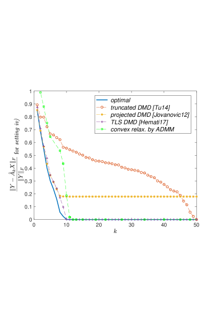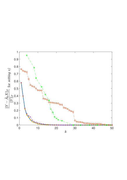
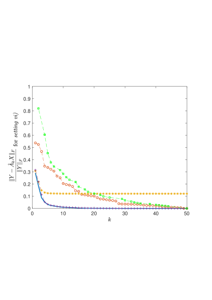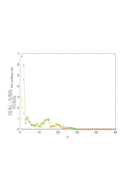
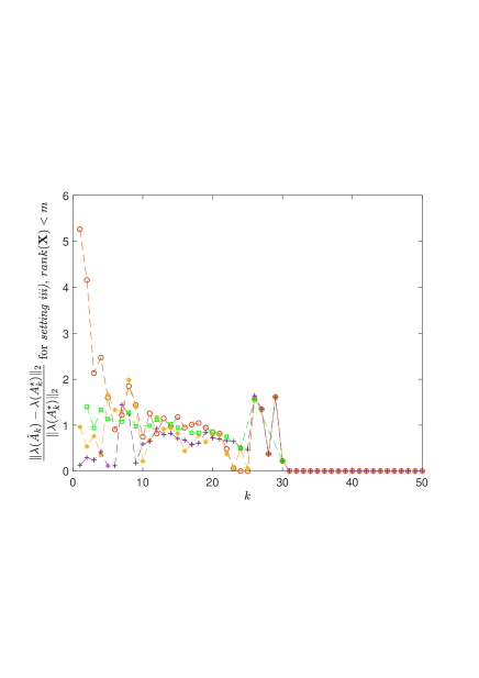
The performance of the different algorithms in terms of reconstruction error is plotted as a function of $k$ in Figure 3 in the case of these three settings. We first comment on results obtained in setting $iv)$. The error obtained by the optimal approximation in this linear setting with $T=2$ appears to vanish for $k\geq d$, i.e., a dimensionality greater than the initial condition dimensionality. This is consistent with Theorem 4.1. Indeed, we know by the definition (15) that $\textrm{rank}(\mathbf{Z})\leq\textrm{rank}({\mathbf{Y}})$; then, dealing with a linear model implies that $\textrm{rank}({\mathbf{Y}})\leq\textrm{rank}({\mathbf{X}})$; as $T=2$ we have $\textrm{rank}({\mathbf{X}})=d$ and therefore $\textrm{rank}(\mathbf{Z})\leq d$ which yields $\sum_{i=d+1}^{m}\sigma_{\mathbf{Z},i}^{2}=0$; in addition we observe that the term $\|{\mathbf{Y}}(I_{m}-\mathbb{P}_{{\mathbf{X}}^{\intercal}})\|_{F}^{2}\approx 2.e-8$ can be neglected in our experiments. It follows from the theorem that the optimal error vanishes for $k\geq d$. The approximation by truncated DMD is associated to an important error which vanishes only for $k=m$, i.e., for a dimensionality equal to the number of snapshots. Concerning the approximation by low-rank projected DMD, it produces a fairly good solution up to $k\leq 8$. However, the approximation becomes clearly sub-optimal for greater dimensions and produces an non-negligible error, even for large values of $k$. TLS DMD yields for $k<10$ an approximation slightly less accurate than the one we propose, while the performances of the two methods are indistinguishable for $k\geq 10$. The approach by convex relaxation produces fairly good results, however with a performance significantly lower than other state-of-the-art methods.

In setting $v)$, we have longer sequences ($T>2$) so that we have $\textrm{rank}({\mathbf{X}})\geq d$. Although the dynamic is linear, no conclusion can be drawn anymore from Theorem 4.1, except that the optimal approximation vanishes for $k\geq m$. However, our optimal approximation yields an error which nearly vanishes for $k\geq d$. This shows that, for this linear model, trajectories concentrate near the subspace spanned by the initial condition. This explains the quasi-optimality of the approximation by low-rank projected DMD, which relies on a strong assumption of linear dependence of snapshots. An approximation by truncated DMD is again clearly sub-optimal and behaves analogously to setting $iv)$. The performance of TLS DMD is in this setting nearly optimal, while convex relaxation is disappointing up to some extent.

In the more realistic geophysical setting $vi)$, we see that the optimal performance achieved by our approximation is far from being reached by approximations by truncated of low-rank projected DMD. Nevertheless, the approximation obtained by TLS DMD is again nearly optimal. As in the linear settings, we observe that the optimal error is small for $k\geq d$. On the other hand, we clearly notice that the assumption used in the approximation by low-rank projected DMD does not hold for this non-linear models and produces an important error, even for large values of $k$. We observe the poor performance of an approximation by truncated DMD or using convex relaxation.

5.3 Robustness to Noise

Figure 4: Error norm as a function of $k$ for setting $vii)$ and $viii)$ using our optimal approximation or state-of-the-art approximations. See details in Section 5.3.

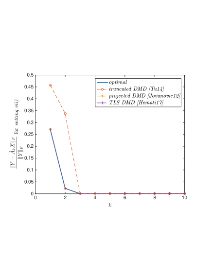Truth
Optimal
Truncated DMD
low-rank Projected DMD
TLS DMD
$\zeta_{1}$		$\zeta_{2}$		$\zeta_{3}$

Figure 5: Amplitudes related to temperature (left columns) and vorticity (right columns) of the right eigenvectors of matrix $F$ of rank $3$ defined in (21): ground truth and estimation obtained in the noisy setting viii) with our optimal approximation, with an approximation by truncated DMD, with an approximation by projected DMD or with an approximation by total-least square DMD. See details in Section 5.3.

In the following, we intend to evaluate the ability of the different methods to extract the eigenvectors in (6) in the presence of noise. To this aim, we build a new dataset of $N=5$ long trajectories with $T=11$ (so that we get $m=50$ snapshots) satisfying (6) with $r=3$. The eigenvectors and eigenvalues in the set $\{(\xi_{i},\zeta_{i},\lambda_{i})\}_{i=1}^{3}$ are computed using Algorithm 2 in the context of setting $vi)$. In other words, matrices ${\mathbf{X}}$ and ${\mathbf{Y}}$ are generated using (1) and the model $f_{t}(x_{t-1})=Fx_{t-1}$ where

$$F=\begin{pmatrix}\zeta_{1}&\zeta_{2}&\zeta_{3}\end{pmatrix}\textrm{diag}(\lambda_{1},\lambda_{2},\lambda_{3})\begin{pmatrix}\xi_{1}&\xi_{2}&\xi_{3}\end{pmatrix}^{\intercal}.$$ (21)

We then consider the two following snapshots configurations:

• setting $vii)$:    the original matrices ${\mathbf{X}}$ and ${\mathbf{Y}}$,

• setting $viii)$:    a noisy version of matrices ${\mathbf{X}}$ and ${\mathbf{Y}}$, where we have corrupted the snapshots with a zero-mean Gaussian noise so that the peak signal-to-noise ratio is $20$ dB.

Results are displayed in Figures 4 and 5. As expected the optimal approximation error vanishes in the noiseless setting in the case where $k\geq r$. We observe only a slight increase of the error in the presence of noise. This shows the robustness of the proposed method. Besides, we remark that the error norm obtained with TLS DMD or with the proposed optimal approach are indistinguishable in both, the noiseless and noisy settings. The approximation by low-rank projected DMD in the noiseless case reproduces almost exactly the optimal behaviour, while its performance slightly deteriorates for $k\geq 2$ in the noisy case. The quasi-optimal performance of this method in the noiseless setting shows that the assumption of linear dependence of snapshots is nearly valid. This assumption no longer holds when snapshots are corrupted by noise. The approximation by truncated DMD is clearly sub-optimal in the noiseless setting. More importantly, the performance of this method becomes dramatic in the presence of noise: the error difference with the optimal one is of the order of more than a decade.

The deterioration is clearly visible in Figure 5. This figure displays the different approximations of eigenvector $\zeta_{3}$ re-arranged in the form of a spatial map. In the presence of noise, the spatial structure of $\zeta_{3}$ is completely rubbed out using an approximation by truncated DMD. Eigenvector $\zeta_{3}$ is fairly recovered using our optimal approximation and roughly estimated using an approximation by low-rank projected DMD. Surprisingly, although TLS DMD yields a quasi-optimal approximation error norm, the structure of eigenvector $\zeta_{3}$ is completely rubbed out, in a very similar manner to low-rank projected DMD.

6 Conclusion

This work shows that we can compute in polynomial time an optimal solution of the non-convex problem related to low-rank linear approximation. As shown in Theorem 4.1, a closed-form solution is in fact the orthogonal projection of the unconstrained problem solution onto a specific low-dimensional subspace. The theorem also provides a closed-form characterization of the optimal approximation error. Based on these results, we show in Proposition 1 that the EVD of this optimal solution can be obtained directly from the snapshots with a complexity of $\mathcal{O}(m^{2}(m+n))$. This off-line complexity is the same as for state-of-the-art sub-optimal methods. Finally, we illustrate through numerical simulations in synthetic and physical setups, the gain brought by using this optimal approximation.

Appendix A Proof of Theorem 4.1

We begin by showing the first part of the theorem, namely that $A_{k}^{\star}={U}_{\mathbf{Z},k}{{U}_{\mathbf{Z},k}}^{\intercal}{\mathbf{Y}}{\mathbf{X}}^{\dagger}$ is a solution of (9). We first prove in this paragraph the existence of a minimizer of (9). Let us show that we can restrict our attention to a minimization problem over the set

$$\mathcal{A}=\{\tilde{A}\in\mathds{R}^{n\times n}:\textrm{rank}(\tilde{A})\leq k,\textrm{Im}(\tilde{A}^{\intercal})\subseteq\textrm{Im}({\mathbf{X}})\}.$$

Indeed, any matrix $A\in\{\tilde{A}\in\mathds{R}^{n\times n}:\textrm{rank}(\tilde{A})\leq k\}$ can be decomposed in two components: $A=A^{\parallel}+A^{\perp}$ where $A^{\parallel}$ belongs to the set $\mathcal{A}$, such that columns of $A^{\parallel}$ are orthogonal to those of $A^{\perp}$, i.e., $A^{\perp}(A^{\parallel})^{\intercal}=0$. From this construction, we have that rows of $A^{\perp}$ are orthogonal to rows of ${\mathbf{X}}$. Using this decomposition, we thus have that $\|{\mathbf{Y}}-A{\mathbf{X}}\|_{F}^{2}=\|{\mathbf{Y}}-A^{\parallel}{\mathbf{X}}\|_{F}^{2}$. Moreover, because of this orthogonal property, we have that $\textrm{rank}(A)=\textrm{rank}(A^{\parallel})+\textrm{rank}(A^{\perp})$ so that $\textrm{rank}(A^{\parallel})\leq\textrm{rank}(A)$. In consequence, if $A$ is a minimizer of (9), then $A^{\parallel}$ is also a minimizer since it leads to same value of the cost function and since it is admissible: $\textrm{rank}(A^{\parallel})\leq\textrm{rank}(A)\leq k$. Therefore, it is sufficient to find a minimizer over the set $\mathcal{A}$.

Now, according to the Weierstrass’ theorem (bertsekas1995nonlinear, , Proposition A.8), the existence is guaranteed if the admissible set $\mathcal{A}$ is closed and the objective function $\|{\mathbf{Y}}-A{\mathbf{X}}\|_{F}^{2}$ is coercive. Let us prove these two properties. We first show that $\mathcal{A}$ is closed. According to (hackbusch2012tensor, , Lemma 2.4), the set of low-rank matrices is closed. Moreover, it is well-known that a linear subspace of a normed finite-dimensional vector space is closed (auliac2005mathematiques, , Chapter 7.2), so that the set of matrices $\mathcal{A}=\{\tilde{A}\in\mathds{R}^{n\times n}:\textrm{Im}(\tilde{A}^{\intercal})\subseteq\textrm{Im}({\mathbf{X}})\}$ is closed. Since $\mathcal{A}$ is the intersection of two closed sets, we deduce that $\mathcal{A}$ is closed. Next, we show coercivity. Let us consider the SVD of any $A\in\mathcal{A}$: $A=U_{A}\Sigma_{A}V_{A}^{\intercal}$, where $\Sigma_{A}=\textrm{diag}(\sigma_{A,1}\cdots\sigma_{A,k})$. From the definition of the Frobenius norm, we have for any $A\in\mathcal{A}$, $\|A\|_{F}=(\sum_{i=1}^{k}\sigma_{A,i}^{2})^{1/2}$. We have that $\|A\|_{F}\to\infty$ if a non-empty subset of singular values, say $\{\sigma_{A,j}\}_{j\in\mathcal{J}}$, tend to infinity. Therefore, we have

$$\lim_{\|A\|_{F}\to\infty:A\in\mathcal{A}}\|{\mathbf{Y}}-A{\mathbf{X}}\|_{F}^{2} =\lim_{\|A\|_{F}\to\infty:A\in\mathcal{A}}\|{\mathbf{Y}}\|^{2}_{F}-2\,\textrm{trace}(Y^{\intercal}A{\mathbf{X}})+\|A{\mathbf{X}}\|_{F}^{2},$$

$$=\lim_{\|A\|_{F}\to\infty:A\in\mathcal{A}}\|A{\mathbf{X}}\|_{F}^{2}=\lim_{\|A\|_{F}\to\infty:A\in\mathcal{A}}\|\Sigma_{A}V_{A}^{\intercal}{\mathbf{X}}\|_{F}^{2},$$

$$=\lim_{\sigma_{A,j}\to\infty:A\in\mathcal{A},j\in\mathcal{J}}\sum_{j=1}^{n}\sigma_{A,j}^{2}\|{\mathbf{X}}^{\intercal}v_{A}^{j}\|_{2}^{2}=\infty.$$

The second equality is obtained because the dominant term when $\|A\|_{F}\to\infty$ is the quadratic one $\|A{\mathbf{X}}\|_{F}^{2}$. The third equality follows from the invariance of the Frobenius norm to unitary transforms while the last equality is obtained noticing that $\|{\mathbf{X}}^{\intercal}v_{A}^{j}\|_{2}\neq 0$ because $v_{A}^{j}\in\textrm{Im}({\mathbf{X}})$ since $A\in\mathcal{A}$. This shows that the objective function is coercive over the closed set $\mathcal{A}$. Thus, using the Weierstrass’ theorem, this shows the existence of a minimizer of (9) in $\mathcal{A}$ and thus in $\{\tilde{A}\in\mathds{R}^{n\times n}:\textrm{rank}(\tilde{A})\leq k\}$. We will no longer restrict our attention to the domain $\mathcal{A}$ in the following and come back to the original problem (9) implying the set of low-rank matrices.

Next, problem (9) can be rewritten as the unconstrained minimization

$$A_{k}^{\star}\in \operatorname*{arg\,min}_{A=PQ^{\intercal}:P,Q\in\mathds{R}^{n\times k}}\|{\mathbf{Y}}-A{\mathbf{X}}\|^{2}_{F}.$$ (22)

In the following we will use the first-order optimality condition of problem (22) to characterize its minimizers. A closed-form expression for a minimizer will then be obtained be introducing an additional orthonormal property. The first-order optimality condition and the additional orthonormal property are presented in the following lemma, which is proven in Appendix B.

Lemma 1

Problem (22) admits a solution such that

$$P^{\intercal}P=I_{k}$$ (23)

$${\mathbf{X}}{\mathbf{Y}}^{\intercal}P={\mathbf{X}}{\mathbf{X}}^{\intercal}Q.$$ (24)

To find a closed-form expression of a minimizer of (22), we need to rewrite condition (24). We prove that this condition is equivalent to

$$\mathbb{P}_{{\mathbf{X}}^{\intercal}}{\mathbf{Y}}^{\intercal}P={\mathbf{X}}^{\intercal}Q.$$ (25)

Indeed, we show by contradiction that (24) implies that, for any solution of the form $PQ^{\intercal}$, there exists $Z\in\mathds{R}^{m\times k}$ such that

$$\mathbb{P}_{{\mathbf{X}}^{\intercal}}{\mathbf{Y}}^{\intercal}P+Z={\mathbf{X}}^{\intercal}Q,$$ (26)

with columns of $Z$ in $\ker({\mathbf{X}})$. Indeed, if $\mathbb{P}_{{\mathbf{X}}^{\intercal}}{\mathbf{Y}}^{\intercal}P+Z\neq{\mathbf{X}}^{\intercal}Q$, then by multiplying both sides on the left by ${\mathbf{X}}$ we obtain $\mathbb{P}_{{\mathbf{X}}}{\mathbf{X}}{\mathbf{Y}}^{\intercal}P+{\mathbf{X}}Z=\mathbb{P}_{{\mathbf{X}}}{\mathbf{X}}{\mathbf{Y}}^{\intercal}P\neq{\mathbf{X}}{\mathbf{X}}^{\intercal}Q$. Since $\mathbb{P}_{{\mathbf{X}}}$ is the orthogonal projector onto the subspace spanned by the columns of ${\mathbf{X}}$, the latter relation implies that ${\mathbf{X}}{\mathbf{Y}}^{\intercal}P\neq{\mathbf{X}}{\mathbf{X}}^{\intercal}Q$ which contradicts (24). This proves that (24) implies (26).

Now, since columns of the two terms in the left-hand side of (26) are orthogonal and since columns of the matrix in the right-hand side are in the image of ${\mathbf{X}}^{\intercal}$, we deduce that the only admissible choice is $Z$ with columns belonging both to $\ker({\mathbf{X}})$ and $\textrm{Im}({\mathbf{X}}^{\intercal})$, i.e., $Z$ is a matrix full of zeros. Therefore, we obtain the necessary condition (25).

We have shown on the one hand that (24) implies (25). On the other hand, by multiplying on the left both sides of (25) by ${\mathbf{X}}$, we obtain (24) (${\mathbf{X}}\mathbb{P}_{{\mathbf{X}}^{\intercal}}={\mathbf{X}}$ because ${\mathbf{X}}{\mathbf{X}}^{\dagger}$ is the orthogonal projector onto the space spanned by the columns of ${\mathbf{X}}$). Therefore the necessary conditions (24) and (25) are equivalent.

We are now ready to characterize a minimizer of (9). According to Lemma 1, we have

$$\min_{A\in\mathds{R}^{n\times n}:\textrm{rank}(A)\leq k} \|{\mathbf{Y}}-A{\mathbf{X}}\|_{F}^{2}$$

$$= \min_{(\tilde{P},\tilde{Q})\in\mathds{R}^{n\times k}\times\mathds{R}^{n\times k}}\|{\mathbf{Y}}-\tilde{P}\tilde{Q}^{\intercal}{\mathbf{X}}\|_{F}^{2}\quad s.t.\quad\left\{\begin{aligned} &\tilde{P}^{\intercal}\tilde{P}=I_{k}\\ &{\mathbf{X}}{\mathbf{Y}}^{\intercal}\tilde{P}={\mathbf{X}}{\mathbf{X}}^{\intercal}\tilde{Q}\\ \end{aligned}\right.,$$ (27)

$$= \min_{(\tilde{P},\tilde{Q})\in\mathds{R}^{n\times k}\times\mathds{R}^{n\times k}}\|{\mathbf{Y}}-\tilde{P}\tilde{Q}^{\intercal}{\mathbf{X}}\|_{F}^{2}\quad s.t.\quad\left\{\begin{aligned} &\tilde{P}^{\intercal}\tilde{P}=I_{k}\\ &\mathbb{P}_{{\mathbf{X}}^{\intercal}}{\mathbf{Y}}^{\intercal}\tilde{P}={\mathbf{X}}^{\intercal}\tilde{Q}\\ \end{aligned}\right.,$$

$$= \min_{\tilde{P}\in\mathds{R}^{n\times k}}\|{\mathbf{Y}}-\tilde{P}\tilde{P}^{\intercal}{\mathbf{Y}}\mathbb{P}_{{\mathbf{X}}^{\intercal}}\|_{F}^{2}\quad s.t.\quad\tilde{P}^{\intercal}\tilde{P}=I_{k},$$ (28)

$$= \min_{\tilde{P}\in\mathds{R}^{n\times k}}\|({\mathbf{Y}}-\tilde{P}\tilde{P}^{\intercal}{\mathbf{Y}})\mathbb{P}_{{\mathbf{X}}^{\intercal}}+{\mathbf{Y}}(I_{m}-\mathbb{P}_{{\mathbf{X}}^{\intercal}})\|_{F}^{2}\quad s.t.\quad\tilde{P}^{\intercal}\tilde{P}=I_{k},$$

$$= \min_{\tilde{P}\in\mathds{R}^{n\times k}}\|\mathbf{Z}-\tilde{P}\tilde{P}^{\intercal}\mathbf{Z}\|_{F}^{2}+\|{\mathbf{Y}}(I_{m}-\mathbb{P}_{{\mathbf{X}}^{\intercal}})\|_{F}^{2}\quad s.t.\quad\tilde{P}^{\intercal}\tilde{P}=I_{k}.$$ (29)

The second equality is obtained from the equivalence between (24) and (25). The third equality is obtained by introducing the second constraint in the cost function and noticing that projection operators are always symmetric, i.e., $(\mathbb{P}_{{\mathbf{X}}^{\intercal}})^{\intercal}=\mathbb{P}_{{\mathbf{X}}^{\intercal}},$ while the last equality follows from the definition of $\mathbf{Z}$ given in (15) and the orthogonality of the columns of the two terms. Problem (29) is a proper orthogonal decomposition problem with the snapshot matrix $\mathbf{Z}$. The solution of this proper orthogonal decomposition problem is the matrix ${U}_{\mathbf{Z},k}$ (with orthonormal columns) defined in Section 4.1, see e.g.,  (quarteroni2015reduced, , Proposition 6.1). We thus obtain from (28) that

$$\min_{A\in\mathds{R}^{n\times n}:\textrm{rank}(A)\leq k}\|{\mathbf{Y}}-A{\mathbf{X}}\|_{F}^{2}=\|{\mathbf{Y}}-{U}_{\mathbf{Z},k}{{U}_{\mathbf{Z},k}}^{\intercal}{\mathbf{Y}}\mathbb{P}_{{\mathbf{X}}^{\intercal}}\|_{F}^{2}=\|{\mathbf{Y}}-\mathbb{P}_{\mathbf{Z},k}{\mathbf{Y}}\mathbb{P}_{{\mathbf{X}}^{\intercal}}\|_{F}^{2}.$$ (30)

Furthermore, we verify that $A_{k}^{\star}={U}_{\mathbf{Z},k}{W}^{\intercal}$ with ${W}=({\mathbf{X}}^{\intercal})^{\dagger}{\mathbf{Y}}^{\intercal}{U}_{\mathbf{Z},k}$ is a minimizer of (22). Indeed, since ${\mathbf{X}}{\mathbf{X}}^{\intercal}{W}={\mathbf{X}}{\mathbf{X}}^{\intercal}({\mathbf{X}}^{\intercal})^{\dagger}{\mathbf{Y}}^{\intercal}{U}_{\mathbf{Z},k}={\mathbf{X}}{\mathbf{Y}}^{\intercal}{U}_{\mathbf{Z},k}$, we check that $({U}_{\mathbf{Z},k},{W})$ is admissible for problem (27). We also check using (25) that $\|{\mathbf{Y}}-{U}_{\mathbf{Z},k}{W}^{\intercal}{\mathbf{X}}\|_{F}^{2}=\|{\mathbf{Y}}-\mathbb{P}_{\mathbf{Z},k}{\mathbf{Y}}\mathbb{P}_{{\mathbf{X}}^{\intercal}}\|_{F}^{2},$ i.e., that $({U}_{\mathbf{Z},k},{W})$ reaches the minimum given in (30). In consequence, we have shown that problem (22), and equivalently problem (9), admit the minimizer $A_{k}^{\star}={U}_{\mathbf{Z},k}{W}^{\intercal}=\mathbb{P}_{\mathbf{Z},k}{\mathbf{Y}}{\mathbf{X}}^{\dagger}$.

It remains to prove the second part of the theorem, namely the characterization of the approximation error. The sought result follows from standard proper orthogonal decomposition analysis. Indeed, according to (quarteroni2015reduced, , Proposition 6.1) the first term of the cost function in (29) evaluated at $A_{k}^{\star}$ is $\|\mathbf{Z}-\mathbb{P}_{\mathbf{Z},k}\mathbf{Z}\|_{F}^{2}=\sum_{i=k+1}^{m}\sigma_{\mathbf{Z},i}^{2}.$

Appendix B Proof of Lemma 1

We begin by proving that any minimizer of (22) can be rewritten as $PQ^{\intercal}$ where $P^{\intercal}P=I_{k}$. Indeed, the existence of the SVD of $\tilde{A}$ for any minimizer $\tilde{A}\in\mathds{R}^{n\times n}$ guarantees that

$$\|{\mathbf{Y}}-\tilde{A}{\mathbf{X}}\|^{2}_{F}=\|{\mathbf{Y}}-U_{\tilde{A}}\Sigma_{\tilde{A}}V^{\intercal}_{\tilde{A}}{\mathbf{X}}\|^{2}_{F},$$

where $U_{\tilde{A}}\in\mathds{R}^{n\times k}$ possesses orthonormal columns. Making the identification $P=U_{\tilde{A}}$ and $Q=V_{\tilde{A}}\Sigma_{\tilde{A}}$ we verify that $\|{\mathbf{Y}}-\tilde{A}{\mathbf{X}}\|^{2}_{F}=\|{\mathbf{Y}}-PQ^{\intercal}{\mathbf{X}}\|^{2}_{F}$ and that $P$ possesses orthonormal columns. Next, any solution $PQ^{\intercal}$ of (22) should satisfy the first-order optimality condition with respect to the $j$-th column denoted $q_{j}$ of matrix $Q$, that is

$$2[-{\mathbf{X}}{\mathbf{Y}}^{\intercal}p_{j}+\sum_{i=1}^{k}(p_{i}^{\intercal}p_{j}){\mathbf{X}}{\mathbf{X}}^{\intercal}q_{i}]=0,$$

where the $j$-th column of matrix $P$ is denoted $p_{j}$. In particular, a solution with $P$ possessing orthonormal columns should satisfy ${\mathbf{X}}{\mathbf{Y}}^{\intercal}p_{j}={\mathbf{X}}{\mathbf{X}}^{\intercal}q_{j},$ or in matrix form ${\mathbf{X}}{\mathbf{Y}}^{\intercal}P={\mathbf{X}}{\mathbf{X}}^{\intercal}Q.\quad\square$

Appendix C Proof of Proposition 1

We have $A_{k}^{\star}=\mathbb{P}_{\mathbf{Z},k}{\mathbf{Y}}{\mathbf{X}}^{\dagger}={U}_{\mathbf{Z},k}{W}^{\intercal}$ which implies that

$${W}^{\intercal}{U}_{\mathbf{Z},k}={{U}_{\mathbf{Z},k}}^{\intercal}{\mathbf{Y}}{\mathbf{X}}^{\dagger}{U}_{\mathbf{Z},k}={{U}_{\mathbf{Z},k}}^{\intercal}\mathbb{P}_{\mathbf{Z},k}{\mathbf{Y}}{\mathbf{X}}^{\dagger}{U}_{\mathbf{Z},k}={{U}_{\mathbf{Z},k}}^{\intercal}{U}_{\mathbf{Z},k}{W}^{\intercal}{U}_{\mathbf{Z},k}.$$

Using the definition of $\zeta_{i}$’s and $\xi_{i}$’s in (20), since the $w^{r}_{i}$’s and $w^{\ell}_{i}$’s are the right and left eigenvectors of ${W}^{\intercal}{U}_{\mathbf{Z},k}$, we verify that

$$A^{\star}_{k}\zeta_{i}={U}_{\mathbf{Z},k}{W}^{\intercal}{U}_{\mathbf{Z},k}w^{r}_{i}={U}_{\mathbf{Z},k}\lambda_{i}w^{r}_{i}=\lambda_{i}\zeta_{i},$$

and that

$$(A^{\star}_{k})^{\intercal}\xi_{i}=\hat{Q}{{U}_{\mathbf{Z},k}}^{\intercal}{W}w^{\ell}_{i}={W}\lambda_{i}w^{\ell}_{i}=\lambda_{i}\xi_{i}.$$

Finally, $\xi_{i}^{\intercal}\zeta_{i}=1$ is a sufficient condition so that $\xi_{i}^{\intercal}A_{k}^{\star}\zeta_{i}=\lambda_{i}.\quad\square$