Enhancing thermoelectric performance using nonlinear transport effects

Abstract

We study nonlinear transport effects on the maximum efficiency and power for both inelastic and elastic thermoelectric generators. The former refers to phonon-assisted hopping in double quantum-dots, while the latter is represented by elastic tunneling through a single quantum-dot. We find that nonlinear thermoelectric transport can lead to enhanced efficiency and power for both types of devices. A comprehensive survey of various quantum-dot energy, temperature, and parasitic heat conduction reveals that the nonlinear transport induced improvements of the maximum efficiency and power are overall much more significant for inelastic devices than the elastic devices, even for temperature biases as small as $T_{h}=1.2T_{c}$ ($T_{h}$ and $T_{c}$ are the temperatures of the hot and cold reservoirs, respectively). The underlying mechanism is revealed as due to the fact that, unlike the Fermi distribution, the Bose distribution is not bounded when the temperature bias increases. A large flux density of absorbed phonons leads to great enhancement of the electrical current, the output power, and the energy efficiency, dominating over the concurrent increase of the parasitic heat current. Our study reveals that nonlinear transport effects can be a useful tool for improving thermoelectric performance.

I Introduction

Thermoelectric energy conversion is important both for fundamental research on, e.g., the physics of mesoscopic electron systemsjoe and for applicationsbook . Advancements in material sciences and nanotechnology have been pushing the frontiers of thermoelectric researches. Nanostructured bulk thermoelectric materialshicks ; nano1 ; nano2 have yielded a (device) figure of merit as high as $ZT\simeq 1.34$kanatzidis ; ncomm , reaching to $\simeq$28% of the Carnot efficiency. In the past few years, studies on inelastic thermoelectricity opened a unprecedented avenue for potential high-performance thermoelectricsjoe1 ; sanchez1 ; jiang1 ; o0 ; DS ; sanchez2 ; magnon ; jiang2 ; pn ; o1 ; sanchez3 ; jordan ; o2 ; 3tjap ; jiang4 ; nonlinear ; jiang5 ; o3 ; felix ; o4 ; exp1 ; exp2 ; exp3 ; lijie ; rev . For an inelastic thermoelectric generator, the input heat is supplied in the form of phonons or other bosons that assist the inelastic transportjiang1 ; rev . As a consequence, the figure of merit can be written aspn ; rev

$$ZT=\frac{\langle\omega\rangle^{2}}{\langle\omega^{2}\rangle-\langle\omega\rangle^{2}+\Delta},$$ (1)

where $\omega$ is the energy of the bosons (throughout this paper we set $\hbar\equiv 1$). Here the average is weighted by the contribution of each inelastic transport channel to the electrical conductancepn ; rev . The term $\Delta$ describes the reduction of the figure of merit due to the parasitic heat conductionpn ; rev . Note that elastic transport processes (i.e., $\omega=0$) do not contribute to the inelastic thermoelectricityjiang1 , although they lead to the conventional thermoelectricity.

Inelastic thermoelectricity has several advantages over the conventional thermoelectricity that is based on elastic transport. First, for inelastic thermoelectrics, a large figure of merit can be achieved by a small bandwidth of the bosons that assist the inelastic transportpn , instead of a small bandwidth of electrons as in Mahan and Sofo’s proposal for the conventional thermoelectricityms . The small bandwidth of the bosons that are involved in the inelastic transport processes does not suppress the electrical conductance (unlike in Mahan and Sofo’s proposalzhou ). Significant inelastic transport can be realized in ionic semiconductors where the electron-phonon scattering is very strongkoch ; gan2 . Second, in conventional thermoelectricity, heat and charge are transported in the same direction which makes it rather difficult to improve the figure of merit by reducing the parasitic phonon thermal conductivity while maintaining high electrical conductivityzhou ; book ; nano1 ; nano2 ; kanatzidis . If heat and charge are transported separately, it will be much easier to manipulate the parasitic phonon thermal conductivity and electrical conductivity concurrently in the aim of high-performance thermoelectricspn ; 3tjap . It has been shown that inelastic thermoelectric devices based on $p$-$n$ junctions with very small band gap (e.g., HgCdTe $p$-$n$ junctions with band gap $\simeq 50$ meV)pn or quantum-dots (QDs) arrays3tjap can have rather high figure of merit even when the phonon parasitic heat conductivity is taken into consideration. It was also shown that in these devices, the inelastic thermoelectricity has larger figure of merit and power factor than the conventional thermoelectricity3tjap .

In this work, we show that nonlinear transport effects can further enhance inelastic thermoelectric efficiency and power when the voltage and/or temperature bias is large. Specifically, when the temperature of the phonon bath is increased, the nonlinear thermoelectric transport leads to significant improvement of both the heat-to-work energy efficiency and the output electric power. All these effects are found to be associated with inelastic thermoelectric transport. In contrast, for elastic thermoelectric transport the nonlinear effects lead to marginal improvement or reduction of the maximum efficiency. The effects of parasitic heat conduction in both the inelastic and elastic thermoelectric devices are investigated carefully. We find that the key difference between the elastic (or the “conventional”) and the inelastic thermoelectricity is that at large temperature biases the inelastic thermoelectric currents increase dramatically due to the exponentially large Bose distribution factor. In contrast, the elastic transport currents are limited by the Pauli exclusion principles. In physical terms, inelastic transport currents are proportional to the flux of bosons absorbed by electrons and enhanced by the Bose distribution, whereas the elastic transport currents around the chemical potential are limited by the Fermi distributions. Considering the similarity between the inelastic thermoelectricspn ; rev and solar cellsshockley ; solar ; booksc , our theory may also be regarded as a possible answer to the question why solar cells have much higher record efficiency than thermoelectrics (even with the Carnot efficiency $\eta_{C}$ taking into account, i.e., considering the ratio $\eta/\eta_{C}$)book ; shockley ; solar ; booksc .

Although nonlinear effects in thermoelectric transport have been discussed in previous studies for both elasticn1 ; n2 ; n3 and inelastic transportn1-3t ; n2-3t , it is our focus here to study the effects of the nonlinear transport on the maximum energy efficiency and the maximum output power.

II Double Quantum-Dots Three-Terminal Thermoelectric Transport

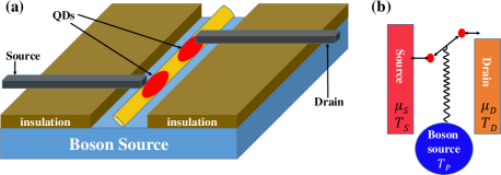
Figure 1: (Color online) (a) Schematic of a double QDs three-terminal thermoelectric device. Two QDs are embedded in a nanowire which is placed on a substrate. The substrate acts as a boson source that emits bosons (e.g., phonons) to assist inelastic hopping between the two QDs. The source electrode (isolated from the substrate by thermally insulating layers) is in contact with one QD, while the drain electrode is in contact with the other QD. The QD connected to the drain has a higher energy than the QD connected to the source. (b) Illustration of the three-terminal inelastic transport. An electron left the source into the first QD (with energy $E_{1}$) hops to the second QD (with a different energy $E_{2}$) as assisted by a boson (e.g., a phonon) from the boson source (with temperature $T_{P}$). The electron then tunnels into the drain electrode from the second QD. Such a process gives inelastic charge transfer from the source to the drain assisted by the boson from the boson source. Both the process and its time-reversal contribute to the inelastic thermoelectricity in the system. The electrochemical potential and temperature of the source (drain) are $\mu_{S}$ and $T_{S}$ ($\mu_{D}$ and $T_{D}$), respectively.

We study the energy efficiency and power for a double-QDs three-terminal thermoelectric device in the nonlinear transport regime. The device is schematically depicted in Fig. 1(a) and explained in the caption. Two QDs, with energy $E_{1}$ and $E_{2}$, are embedded in a nanowire. For simplicity, we consider the situations where there is only one spin-degenerate energy level in each QD relevant for thermoelectric transport. This assumption can be justified for small QDs where the energy level separation in each QD is much larger than $k_{B}T$ganqd . The difference between $E_{1}$ and $E_{2}$ can be tuned by the local potentials of the two QDs. We consider high-temperature transport where the effect of Coulomb interaction is negligible. The electron spin degeneracy doubles the electronic charge and heat currents. The phonon assisted hopping transport is illustrated in Fig. 1(b) and explained in the caption. Besides, electron can also tunnel elastically between the source and the drain via the two QDs. The sequential tunneling processes are suppressed when the energy difference $|E_{2}-E_{1}|$ is significant. A similar system was studied in Ref. nonlinear where thermoelectric rectification and transistor effects were obtained. The double-QDs device is described by the following Hamiltonian

$$H=H_{QD}+H_{ep}+H_{p}+H_{tun}+H_{lead},$$ (2)

where the QDs are described by

$$H_{QD}=E_{1}d_{1}^{\dagger}d_{1}+E_{2}d_{2}^{\dagger}d_{2}+t(d_{1}^{\dagger}d_{2}+d_{2}^{\dagger}d_{1}),$$ (3)

the inter-QD electron-phonon interaction is given by

$$H_{ep}=\sum_{\vec{q}}M_{\vec{q}}d_{1}^{\dagger}d_{2}(a_{\vec{q}}+a_{-\vec{q}}^{\dagger})+{\rm H.c.},$$ (4)

with the phonon Hamiltonian

$$H_{p}=\sum_{\vec{q}}\omega_{\vec{q}}(a_{\vec{q}}^{\dagger}a_{\vec{q}}+\frac{1}{2}).$$ (5)

The tunneling between the QDs and the electrodes are described by

$$H_{tun}=\sum_{\vec{k}}(V_{S,\vec{k}}c_{S,\vec{k}}d_{1}^{\dagger}+V_{D,\vec{k}}c_{D,\vec{k}}d_{2}^{\dagger})+{\rm H.c.},$$ (6)

where the two leads (the source and the drain) have the Hamiltonian,

$$H_{lead}=\sum_{j=S,D}\sum_{\vec{k}}\varepsilon_{j,\vec{k}}c_{j,\vec{k}}^{\dagger}c_{j,\vec{k}}.$$ (7)

Here $d_{i}^{\dagger}$ ($i=1,2$) creates an electron in the $i^{th}$ QD, $c_{S,\vec{k}}^{\dagger}$ and $c_{D,\vec{k}}^{\dagger}$ create electrons in the source and the drain with wavevector $\vec{k}$, respectively. $a_{\vec{q}}^{\dagger}$ creates a phonon with wavevector $\vec{q}$ in the nanowire. For simplicity, the spin index of electrons and the branch index of phonons are omitted in the above equations. $t$ is the tunnel coupling between the two QDs. $M_{\vec{q}}$ is the electron-phonon coupling matrix element. The phonons here should be phonons in the nanowire. We assume that the thermal contact between the nanowire and the substrate is good so that their temperatures are approximately the same (denoted as $T_{P}$). The frequency of the phonon is $\omega_{\vec{q}}$. The tunnel coupling between the first (second) QD and the source (drain) is described by $V_{S,\vec{k}}$ ($V_{D,\vec{k}}$). Both the coupling and the spectrum in the leads $\varepsilon_{j,{\vec{k}}}$ ($j=S,D$) determine the tunneling rate between the electrodes and the QDs. We shall describe the tunneling between the source (drain) and the first (second) QD phenomenologically as an energy-independent constant, $\gamma_{1}$ ($\gamma_{2}$). For simplicity, we consider the situations with $\gamma_{1}=\gamma_{2}=\gamma_{e}$. The tunneling between the first (second) QD and the drain (source) can be obtained by the perturbation theory as [for $t^{2}\ll(E_{2}-E_{1})^{2}$]

$$\gamma_{1}^{\prime}=\gamma_{2}^{\prime}\equiv\gamma_{e}^{\prime}=\frac{t^{2}\gamma_{e}}{(E_{2}-E_{1})^{2}},$$ (8a)

The rate of electron transfer from the first QD to the second QD due to the electron-phonon scattering is given by

$$\Gamma_{12}=\gamma_{ep}[f_{1}(1-f_{2})N_{P}^{+}-f_{2}(1-f_{1})N_{P}^{-}]$$ (9)

where $\gamma_{ep}=2\pi\sum_{\vec{q}}|M_{\vec{q}}|^{2}\delta(|E_{1}-E_{2}|-\omega_{\vec{q}})$ is the electron-phonon scattering rate calculated from the Fermi golden rule. $f_{i}$ ($i=1,2$) are the probabilities of finding an electron on the $i$-th QD. $N_{P}^{\pm}={\rm Abs}(n_{B}[\pm(E_{2}-E_{1})/(k_{B}T_{P})])$ where $n_{B}(x)=1/(e^{x}-1)$ is the Bose distribution function.

This model has been studied before by the authorsjiang1 ; jiang2 ; nonlinear ; rev . Particularly, in Ref. nonlinear , we studied the nonlinear thermoelectric transport in the system and shown that the device can function as cross-correlated thermoelectric rectifications and transistors. One of the remarkable properties of the system is that it allows thermal transistor effect without relying on negative differential thermal conductance, in contrast to common believes. Here we focus on the thermoelectric efficiency and power of the device in the nonlinear regime. While Ref. nonlinear deals with the effects of low-frequency phonons at low temperatures, here we focus on the situations where the phonon energy $\omega$ is close to $k_{B}T_{D}$ ($T_{D}$ is the Debye temperature) for elevated temperatures. There are at least two advantages in this regime: First, the electron-phonon interaction is much stronger, leading to higher current density in the inelastic transport channels; Second, the phonon energy, $\sim k_{B}T_{D}$, is usually higher than $k_{B}T$, which is beneficial for the figure of merit, as indicated by Eq. (1).

There are two electronic and one bosonic reservoirs in our thermoelectric device: the source (with chemical potential $\mu_{S}$ and temperature $T_{S}$), the drain (with chemical potential $\mu_{D}$ and temperature $T_{D}$), and the phonon bath (i.e., the substrate, with temperature $T_{P}$). In this three-terminal device, all reservoirs are isolated using thermal insulation [see Fig. 1(a)]. Energy and charge are transported through the double QDs. Thermodynamic analysis gives the following currents and their conjugated affinities,nonlinear

$$I_{e}=-e\frac{dN_{S}}{dt},\quad A_{e}=\frac{\mu_{S}-\mu_{D}}{e}(\frac{1}{2T_{S}}+\frac{1}{2T_{D}}),$$

$$I_{Q,e}=\frac{1}{2}(\frac{dQ_{D}}{dt}-\frac{dQ_{S}}{dt}),\quad A_{Q,e}=\frac{1}{T_{D}}-\frac{1}{T_{S}},$$

$$Q_{in}=-\frac{dQ_{P}}{dt},\quad A_{in}=\frac{1}{2T_{S}}+\frac{1}{2T_{D}}-\frac{1}{T_{P}}.$$ (10)

Here $e<0$ is the electron charge and $N_{S}$ is the electron number in the source. $Q_{S}$, $Q_{D}$, and $Q_{P}$ represent the heat content [$Q_{i}=E_{i}-\mu_{i}N_{i}$ for $i=S,D$, and $Q_{P}=E_{P}$ where $E_{i}$ ($i=S,D,P$) are the total energy and $N_{i}$ ($i=S,D$) are the total electron number for these reservoirs] for the source, drain, and phonon bath, respectively. In this work, we focus on the situation with $T_{S}=T_{D}\equiv T_{e}$. Thus we have

$$A_{e}=\frac{V}{T_{e}},\quad V\equiv\frac{\mu_{S}-\mu_{D}}{e},$$ (11a)

$$A_{Q,e}=0,\quad A_{in}=\frac{1}{T_{e}}-\frac{1}{T_{P}}.$$ (11b)

The chemical potentials of the source and the drain are set anti-symmetrically around the equilibrium value $\mu\equiv 0$, i.e., $\mu_{S}=eV/2=-\mu_{D}$.

We consider harvesting the heat from the (hot) phonon bath to generate electricity. The energy efficiency is hence

$$\eta=\frac{-I_{e}V}{Q_{in}}\leq\eta_{C}\equiv\frac{T_{h}-T_{c}}{T_{h}},$$ (12)

where $\eta_{C}$ is the Carnot efficiency, $T_{h}=T_{P}$ and $T_{c}=T_{e}$. Both the efficiency $\eta$ and the output power

$$P=-I_{e}V$$ (13)

are of central concern in this work. The heat injected into the system from the boson source (here is the phonon bathjiang1 ) is

$$Q_{in}=I_{Q,ph}+I_{Q,pr},\quad I_{Q,ph}\equiv 2\omega\Gamma_{12},\quad\omega\equiv E_{2}-E_{1}$$

where $I_{Q,pr}$ is the parasitic phonon heat current. The factor of two in the above equation comes from electron spin degeneracy.

The steady-state transport in the three-terminal device is studied via the following rate equations which treat the elastic and inelastic processes on equal footing,

$$0=\frac{df_{1}}{dt}=$$

$$\quad-\gamma_{e}[f_{1}-f_{S}(E_{1})]-\gamma_{e}^{\prime}[f_{1}-f_{D}(E_{1})]-\Gamma_{12},$$ (14a)

$$0=\frac{df_{2}}{dt}=$$

$$\quad-\gamma_{e}[f_{2}-f_{D}(E_{2})]-\gamma_{e}^{\prime}[f_{2}-f_{S}(E_{2})]+\Gamma_{12}.$$ (14b)

By solving the above equations, we can determine the nonequilibrium steady-state distributions on the QDs, $f_{1}$ and $f_{2}$. Afterwards, the electrical and heat currents can be obtained via the following equations (the factor of two originates from electron-spin degeneracy)

$$I_{e}=2e\gamma_{e}[f_{S}(E_{1})-f_{1}]+2e\gamma_{e}^{\prime}[f_{S}(E_{2})-f_{2}],$$ (15a)

$$Q_{in}=2\omega\Gamma_{12}+I_{Q,pr},$$ (15b)

where the parasitic phonon heat current, $I_{Q,pr}$, is calculated via

$$I_{Q,pr}=\int_{0}^{\infty}\frac{dE}{2\pi}E{\cal T}_{pr}(E)[n_{B}(\frac{E}{k_{B}T_{P}})-n_{B}(\frac{E}{k_{B}T_{e}})].$$ (16)

Here ${\cal T}_{pr}(E)$ is the energy-dependent transmission function for phonons. We note that serious considerations of the parasitic heat conduction in the literature are scarce, particularly in the nonlinear regime (Note that a phenomenological heat conductivity parameter cannot include the nonlinear effect). This is mainly because such an effect depends on the details of the device and contacts. Hence it is rather difficult to deduce the transmission function from theoretical aspects (if it is at all possible). To avoid the complexity, we include the parasitic heat conduction via an ideally simple transmission function for phonons transferring between the phonon bath and the source/drain terminals, ${\cal T}_{pr}(E)=\alpha\Theta(E_{cut}-E)$ where $\alpha$ is a dimensionless constant and $E_{cut}$ is the cut-off energy of the phonons. These phonons are not absorbed by electrons and hence do not contribute to the thermoelectric energy conversion. The parameters $\alpha$ and $E_{cut}$ measure the average transmission level and the effective bandwidth of the parasitic phonons, respectively. The parasitic heat current measures how much energy flux carried by the bosons that are not absorbed by the electrons (i.e., not involved in the inelastic transport).

The linear transport coefficients are obtained by calculating the ratios between currents and affinities in the regime with very small voltage bias and temperature difference. In the linear-response regime the current-force relations are

$$I_{i}=\sum_{j}M_{ij}A_{j}$$ (17)

for the charge and heat transports. In the following we will compare the energy efficiency, power, and currents between the full calculation using Eqs. (15) (denoted as “nonlinear” for short) and the calculation using Eq. (17) and assuming its validity for large biases (denoted as “linear” for short).

III Nonlinear transport enhances efficiency and power for inelastic thermoelectric devices

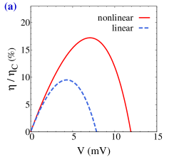
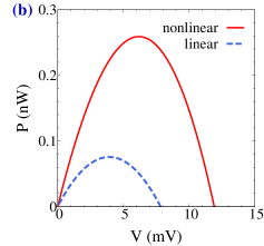
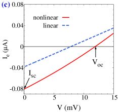
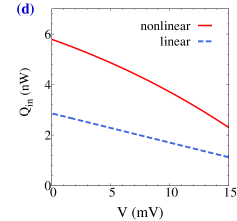
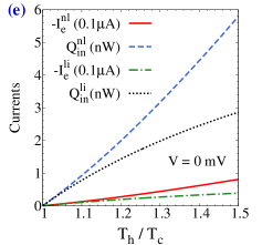
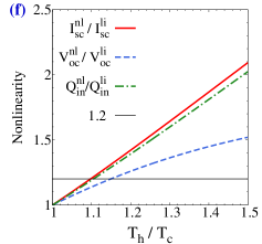
Figure 2: (Color online) Inelastic thermoelectricity. (a) Energy efficiency $\eta$ in units of the Carnot efficiency $\eta_{C}$ and (b) output power $P$ as functions of voltage $V$ (in units of mV). Parameters: $\gamma_{e}=10$ meV, $\gamma_{ep}=5$ meV, $t=10$ meV, $E_{cut}=100$ meV, $T_{h}=225$ K, $T_{c}=150$ K, $\alpha=0.1$, $E_{1}=-E_{2}=-2k_{B}T_{c}$. (c) Electrical and (d) heat currents obtained via full calculation using Eq. (15) (labeled as “nonlinear”) and those calculated via the linear-approximation using Eq.(17) (labeled as “linear”). (e) The electrical currents $I_{e}$ and heat currents $Q_{in}$ as functions of $T_{h}/T_{c}$ for the short-circuit condition $V=0$. Here the superscript “nl” denotes the results from full calculation with nonlinear effects, while the superscript “li” denotes the results from linear-approximation. The same notation of superscript is used in (f) as well. (f) The short-circuit current $I_{sc}$, the open-circuit voltage $V_{oc}$, and the heat current $Q_{in}$ measured by their values in the linear-approximation for various $T_{h}/T_{c}$. The line “1.2” is used to signify considerable nonlinearity.

We calculate the efficiency and output power for a three-terminal inelastic thermoelectric generator. At fixed temperatures $T_{h}$ and $T_{c}$ (with $T_{h}=225$ K and $T_{c}=150$ K), the nonlinear transport yields significant improvement of the maximum efficiency and power, as shown in Figs. 2(a) and 2(b). The maximum efficiency calculated via linear-approximation is only $9.7\%$ of the Carnot efficiency, while the full calculation (including the nonlinear transport effect) leads to a maximum efficiency of $17$% of the Carnot efficiency. The maximum output power increases from 0.08 nW to 0.26 nW, when the nonlinear transport effect is taken into account. The temperatures adopted here is consistent with the experimental fact that large temperature difference is easier to achieve at low temperatureglushk . Nevertheless, our theory also works for high temperatures and give the same conclusions on the nonlinear thermoelectric performance.

To understand the physical origin of the enhancement of the maximum efficiency and power, we first study how the electrical and heat currents are affected by the nonlinear transport effect. From Fig. 2(c) it is seen that the electrical current is considerably enhanced due to the nonlinear effect. Here we adopt two quantities used in the solar cell literaturebooksc to analyze the nonlinear thermoelectric transport: the short-circuit current $I_{sc}$ (i.e., the electrical current at $V=0$) and the open-circuit voltage $V_{oc}$ (i.e., the voltage at which the electrical current vanishes). The product of the two

$${\cal P}\equiv-I_{sc}V_{oc}$$ (18)

characterizes the maximum output powerbooksc . Indeed, the full calculation gives a ${\cal P}$ more than 3 times as large as the ${\cal P}$ obtained from the linear-approximation, agreeing well with the improvement of the maximum power.

To understand the improvement of the maximum efficiency, we also need to examine how the input heat $Q_{in}$ is affected by the nonlinear transport effect. Fig. 2(d) shows that the input heat at $V=0$, $Q_{in}(V=0)$, is increased to about 2 times as large as that obtained via the linear-approximation. The increase of the output power then exceeds that of the input heat, explaining the improvement of the maximum efficiency. The above analysis reveals the importance of the quantities $I_{sc}$, $V_{oc}$, and $Q_{in}(V=0)$ in the study of the maximum power and efficiency, which will also be exploited in the study of the nonlinear transport effect on the performance of the elastic tunneling thermoelectric device later.

The nonlinear transport effect is reflected directly in the dependences of the electrical and heat currents on the temperature ratio $T_{h}/T_{c}$ when $T_{c}$ is fixed, as shown in Fig. 2(e). Both the electrical and heat currents are much enhanced due to the nonlinear transport effect, even for $T_{h}\leq 1.5T_{c}$. To manifest the nonlinear effect more obviously, we shown in Fig. 2(f) the ratio of the short-circuit current obtained via the full calculation (i.e., with the nonlinear transport effect) $I_{sc}^{nl}$ to that obtained via the linear-approximation, $I_{sc}^{li}$, as well as similar ratios for the other two quantities, the open-circuit voltage $V_{oc}$ and the short-circuit heat current $Q_{in}$. It is seen that these ratios increase rapidly with increasing temperature $T_{h}$ when $T_{c}$ is fixed. For $T_{h}\geq 1.1T_{c}$, the nonlinear transport effect is already prominent enough to produce $>20$% deviation between the “nonlinear” and the “linear” currents and voltage. Such enhancement of currents and voltage due to the nonlinear effect is the origin of the significant improvement of the performance of the inelastic thermoelectric generator.

IV Effects of nonlinear transport on efficiency and power for elastic thermoelectric devices

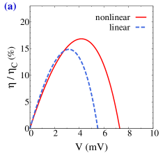
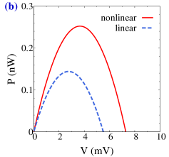
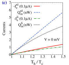
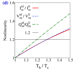
Figure 3: (Color online) Elastic thermoelectricity. (a) Energy efficiency $\eta$ in units of the Carnot efficiency $\eta_{C}$ and (b) output power $P$ as functions of voltage $V$ (in units of mV) for the elastic thermoelectric device. Parameters: $\gamma_{e}=10$ meV, $E_{cut}=100$ meV, $T_{h}=225$ K, $T_{c}=150$ K, $\alpha=0.1$, $E_{0}=2k_{B}T_{c}$. (c) Electrical and heat currents as functions of the temperature ratio $T_{h}/T_{c}$ for the short-circuit condition $V=0$. (d) The short-circuit current $I_{sc}$, the open-circuit voltage $V_{oc}$, and the heat current $Q_{in}$ measured by their values in the linear-approximation vs. $T_{h}/T_{c}$. The line “1.2” is used to signify considerable nonlinearity. The quantities from the full calculation (i.e., with nonlinear effects) are labeled by the superscript “nl”, while those from the linear-approximation are denoted by the superscript “li”.

As a comparison, we also study the nonlinear transport effects on the performance of elastic thermoelectric devices. A simple candidate of such devices is a two-terminal QD thermoelectric device, i.e., a QD connected with the source (of temperature $T_{h}$) and the drain (of temperature $T_{c}<T_{h}$) electrodes via resonant tunneling. We adopt parameters comparable with those in the previous section: the tunneling rate between the QD and the source (drain) is $\gamma_{e}=10$ meV and the QD energy is $E_{0}=2k_{B}T_{c}$. There is parasitic phonon heat conduction between the source and the drain as described by Eq. (16) and characterized by the two parameters, $\alpha=0.1$ and $E_{cut}=100$ meV.

We calculate the electrical and heat currents using the Landauer formula with the energy-dependent transmission function

$${\cal T}_{e}(E)=\frac{\gamma_{e}^{2}}{(E-E_{0})^{2}+\gamma_{e}^{2}}.$$ (19)

The currents are given by

$$I_{e}=e\int\frac{dE}{2\pi}{\cal T}_{e}(E)[f_{S}(E)-f_{D}(E)],$$ (20a)

$$I_{Q,e}=\int\frac{dE}{2\pi}(E-\mu_{S}){\cal T}_{e}(E)[f_{S}(E)-f_{D}(E)],$$ (20b)

$$Q_{in}=I_{Q,e}+I_{Q,pr},$$ (20c)

The energy efficiency and output power can be obtained using the above currents.

As shown in Figs. 3(a) and 3(b), the maximum efficiency for the elastic thermoelectric device within the linear-approximation [i.e., Eq. (17)], is 15% of the Carnot efficiency and the maximum power is 0.14 nW. Both of them are larger than those of the inelastic thermoelectric device under the linear-approximation. However, here the nonlinear transport effect only leads to marginal improvement of the maximum efficiency and power: the efficiency is increased only to 17% of the Carnot efficiency, while the maximum power is raised only to 0.25 nW. Judging from the linear-response thermoelectric transport coefficients and the figure of merit (which is well-defined for the linear-response regime), the elastic thermoelectric device has much higher efficiency and power than the inelastic thermoelectric device. However, in the nonlinear transport regime, the inelastic thermoelectric device has the same maximum efficiency and larger maximum power. The nonlinear transport effect leads to much strong enhancement of the maximum efficiency and power for the inelastic device as compared to the elastic device.

To further explore the nonlinear effects in thermoelectric transport in the elastic tunneling device, we plot the short-circuit electrical and heat currents as functions of $T_{h}/T_{c}$ in Fig. 3(c). The results here indicate that the enhancement of the electrical and heat currents due to the nonlinear transport effect is much weakened for the elastic device, as compared to the inelastic device. Fig. 3(d) shows that to achieve 20% deviation between the “nonlinear” and the “linear” electrical currents, $T_{h}$ must be greater than $1.2T_{c}$. The overall increment of the currents and voltage due to the nonlinear transport effect is much reduced here, as compared to the inelastic device.

These results are in fact consistent with the findings in the literature. In Ref. robust , it was found that the linear-transport approximation is robust for a range of temperature biases in resonant tunneling QD thermoelectric devices.

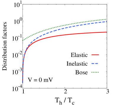
Figure 4: (Color online) Distribution factor that determines the magnitude of the charge and heat currents in the resonant-tunneling QD device (red solid curve, labeled as “Elastic”), that for the inelastic hopping transport in the three-terminal device (blue dashed curve, labeled as “Inelastic”), and the Bose-Einstein distribution factor $n_{B}(|E_{2}-E_{1}|/k_{B}T_{h})$ for the inelastic hopping transport in the three-terminal device (green dotted curve, labeled as “Bose”). Parameters: $E_{0}=2k_{B}T_{c}$, $E_{1}=-E_{2}=-2k_{B}T_{c}$, $\mu_{S}=\mu_{D}=0$ (i.e., $V=0$). For the two-terminal elastic device, $T_{S}=T_{h}$ and $T_{D}=T_{c}$, whereas for the three-terminal inelastic device, $T_{S}=T_{D}=T_{c}$ and $T_{P}=T_{h}$. The distribution factors are adjusted so that the “elastic” and “inelastic” curves start at the same value for very small $T_{h}/T_{c}-1$.

V Distinction between inelastic and elastic thermoelectricity from the distribution factor

To understand the underlying mechanism that leads to the distinction between the elastic and the inelastic thermoelectric energy conversions. We study the distribution factors which crucially determines the magnitude of the charge current and a part of the heat current. For the two-terminal elastic thermoelectric transport the charge and heat currents are dominated by the Fermi-Dirac distribution factor of $f_{S}(E_{0})-f_{D}(E_{0})$ with $T_{S}=T_{h}$ and $T_{D}=T_{c}$. For the three-terminal inelastic thermoelectric transport the currents are determined by the distribution factor, $f_{1}(1-f_{2})N_{P}^{+}-f_{2}(1-f_{1})N_{P}^{-}$ with $T_{S}=T_{D}=T_{c}$ and $T_{P}=T_{h}$, which is a mixture of Fermi-Dirac and Bose-Einstein distributions. When $\gamma_{e}\gg\Gamma_{12}$nonlinear , we can adopt the approximation $f_{1}\simeq f_{S}(E_{1})$, $f_{2}\simeq f_{D}(E_{2})$, and calculate the distribution factor $f_{1}(1-f_{2})N_{P}^{+}-f_{2}(1-f_{1})N_{P}^{-}$ easily. We plot the distribution factors for the elastic and inelastic devices together in Fig. 4. We have adjusted their values so that they are equal when $T_{h}/T_{c}-1$ is very small. Fig. 4 shows that the distribution factor for the elastic device saturates at large temperature bias, whereas the distribution factor for the inelastic device does not. The saturation of the distribution factor for the elastic transport is understandable, since there is a strict bound on the distribution factor $|f_{S}(E_{0})-f_{D}(E_{0})|\leq 1$, due to the Pauli exclusion principle. In contrast, there is no bound on the distribution factor for the inelastic transport. In fact, the Bose-Einstein distribution $N_{P}^{+}=1/[\exp(\frac{E_{2}-E_{1}}{k_{B}T_{h}})-1]$ is not bounded (see the dotted curve in Fig. 8). This term dominates the rapid growth of the inelastic distribution factor when the temperature ratio $T_{h}/T_{c}$ is large. This observation explains well the distinction between the nonlinear effects in the elastic and inelastic devices.

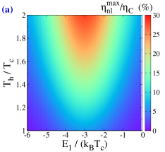
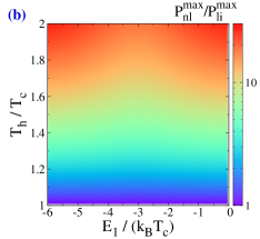
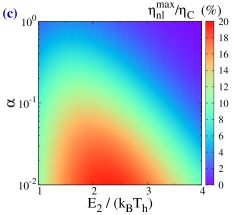
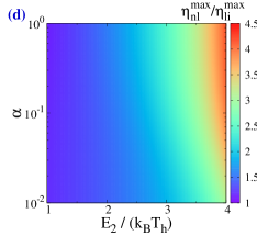
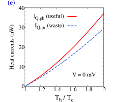
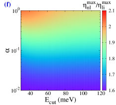
Figure 5: (Color online) Inelastic thermoelectricity. (a) Energy efficiency $\eta_{nl}^{max}/\eta_{C}$ and (b) power ratio $P^{max}_{nl}/P^{max}_{li}$ vs. QD energy $E_{1}$ (in unit of $k_{B}T_{c}$) and the temperature of the phonon bath $T_{P}=T_{h}$ for $E_{2}=E_{1}+6k_{B}T_{c}$ with $T_{c}=150$ K. Here the quantities obtained via full calculation are denoted by the subscript “nl”, whereas those obtained via linear-approximation are labeled by the subscript “li”. (c) The energy efficiency $\eta_{nl}^{max}/\eta_{C}$ and (d) the ratio $\eta_{nl}^{max}/\eta_{li}^{max}$ vs. the QD energy with $E_{2}=-E_{1}$ (in unit of $k_{B}T_{h}$) and the parasitic heat conduction (controlled by $\alpha$) for $T_{h}=1.2T_{c}=180$ K and $T_{c}=150$ K. (e) The useful thermoelectric heat current $I_{Q,ph}$ and the waste parasitic heat current $I_{Q,pr}$ as functions of temperature ratio $T_{h}/T_{c}$ for $E_{2}=-E_{1}=3k_{B}T_{c}$ and $V=0$. (f) The ratio $\eta_{nl}^{max}/\eta_{li}^{max}$ vs. the parasitic heat conduction parameters $\alpha$ and $E_{cut}$ for $T_{h}=1.2T_{c}=180$ K ($T_{c}=150$ K) and $E_{2}=-E_{1}=3k_{B}T_{c}$. The Other parameters are $\gamma_{e}=10$ meV, $\gamma_{ep}=5$ meV, and $t=10$ meV.

VI Variation of temperature bias, quantum-dot energy, and parasitic heat conduction

In the above, by focusing on two specific examples, we have illustrated the essential difference between inelastic and elastic thermoelectric devices in the nonlinear transport regime. We revealed the crucial roles of the Bose and Fermi distributions in the nonlinear energy efficiency in these two types of thermoelectric devices. To avoid being misled by particular choice of parameters, in this section we study the effects of nonlinear transport on thermoelectric energy efficiency and output power for various temperatures, QD energies, and parasitic heat conduction.

We first study how the inelastic thermoelectric efficiency varies with these parameters. In Fig. 9(a), we show the ratio of the maximum efficiency over the Carnot efficiency $\eta_{max}/\eta_{C}$ for various the temperature $T_{h}=T_{P}$ and QD energy $E_{1}$ when the energy difference $E_{2}-E_{1}$ is fixed to $6k_{B}T_{c}$. For each configuration, the energy efficiency is optimized by varying the voltage $V$. If the linear-approximation is valid for all $T_{h}$, then the ratio $\eta_{max}/\eta_{C}$ should not vary with the temperature ratio $T_{h}/T_{c}$. The dependence of the ratio $\eta_{max}/\eta_{C}$ on $T_{h}/T_{c}$ directly reflects the nonlinear transport effect. Fig. 5(a) indicates that the nonlinear effect on the maximum efficiency is prominent: for $E_{1}\simeq-3k_{B}T_{c}=-E_{2}$, the maximum efficiency can increase from 6% to about 27%! Combining with previous studies on inelastic thermoelectricity3tjap ; jordan , we conclude that the “particle-hole symmetric” configuration $E_{2}=-E_{1}$ is the optimal configuration for inelastic thermoelectricity in both linear and nonlinear transport regimes.

The enhancement of the maximum power due to the nonlinear transport effect, $P^{max}_{nl}/P^{max}_{li}$, is also calculated for various QD energies and temperatures [results shown in Fig. 5(b)]. Here the enhancement factor, $P^{max}_{nl}/P^{max}_{li}$, can be as large as 30. The significant enhancement of the maximum power with increasing temperature $T_{h}$ is the driving force for the prominent improvement of the maximum efficiency shown in Fig. 5(a). Noticeable improvement ($\sim 70\%$) of the maximum power can already be achieved at $T_{h}/T_{c}$ as small as 1.1. Beside the rapid increase with the temperature $T_{h}$, the enhancement of the maximum power showed no considerable dependence on the QD energy.

Under the consideration that smaller temperature biases are probably more attainableglushk , we also study the maximum efficiency and its enhancement at $T_{h}-T_{c}=0.2T_{c}$ with $T_{c}=150$ K for the “particle-hole symmetric” configuration $E_{2}=-E_{1}$. The results in Fig. 5(c) indicate that the energy efficiency is optimized for small $\alpha$ and $E_{2}\simeq 2.5k_{B}T_{h}$. This result is slightly different from the previous results of $E_{2}=-E_{1}\simeq 3k_{B}T_{c}$ for the optimization of energy efficiency in the linear-response regimejordan ; n1-3t ; 3tjap .

We further explore the enhancement of the maximum efficiency due to the nonlinear transport effect for the “particle-hole symmetric” configuration $E_{2}=-E_{1}$. The enhancement of the maximum efficiency is characterized by the ratio $\eta^{max}_{nl}/\eta^{max}_{li}$ in Fig. 5(d) (subscripts “nl” and “li” denote the full calculation with the nonlinear effect and the linear-approximation, respectively). The enhancement factor $\eta^{max}_{nl}/\eta^{max}_{li}$ can reach close to 3 even for a small temperature bias $T_{h}-T_{c}=0.2T_{c}$ with $T_{c}=150$ K. Such enhancement is more prominent for large $E_{2}$. We find that this is because the useful thermoelectric heat current surpasses the waste parasitic heat current more significantly when the QD energy $E_{2}=-E_{1}$ is large. As shown in Fig. 5(e) for one typical case, the useful heat current increases faster than the waste heat current with increasing temperature bias, i.e., the parasitic heat conduction becomes less and less important with increasing temperature bias. Since the enhancement of the thermoelectric heat current $I_{Q,ph}=2(E_{2}-E_{1})\Gamma_{12}$ increases substantially with $E_{2}$, the improvement of the maximum efficiency is more prominent for large $E_{2}$.

The results in Fig. 5(f) show that the parameter $E_{cut}$ affect the enhancement of energy efficiency much weaker than the other parameter $\alpha$. This result is consistent with the physics picture that the tunneling heat conduction is dominated by the energy scale around $k_{B}T_{h}\simeq 15$ meV. Fig. 5(f) indicates that considerable improvement of thermoelectric efficiency can be achieved for a large parameter region even for the small temperature bias $T_{h}-T_{c}=0.2T_{c}$.

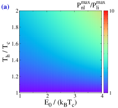
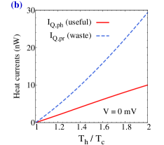
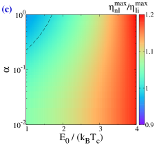
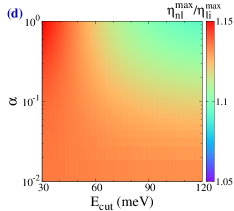
Figure 6: (Color online) Elastic thermoelectricity. (a) The ratio of the maximum powers $P^{max}_{nl}/P^{max}_{li}$ as a function of the QD energy $E_{0}$ (in unit of $k_{B}T_{c}$) and the temperature ratio $T_{h}/T_{c}$ for $T_{c}=150$ K. Here the quantities obtained via the full calculation (including the nonlinear effect) are labeled with the subscript “nl”, whereas those obtained via the linear-approximation is denoted with the subscript “li”. (b) The useful thermoelectric heat current $I_{Q,e}$ and the waste parasitic heat current $I_{Q,pr}$ vs. the temperature ratio $T_{h}/T_{c}$ for $E_{0}=3k_{B}T_{c}$, $T_{c}=150$ K, and $V=0$. (c) The ratio $\eta_{nl}^{max}/\eta_{li}^{max}$ as a function of the QD energy $E_{0}$ and the parasitic heat conduction parameter $\alpha$ for $T_{h}=1.2T_{c}=180$ K ($T_{c}=150$ K) and $E_{cut}=100$ meV. The black-dashed curve represents the contour of $\eta_{nl}^{max}/\eta_{li}^{max}=1$. (d) The ratio $\eta_{nl}^{max}/\eta_{li}^{max}$ vs. the parasitic heat conduction parameters $\alpha$ and $E_{cut}$ for $T_{h}=1.2T_{c}=180$ K ($T_{c}=150$ K) and $E_{0}=3k_{B}T_{c}$. For all figures here $\gamma_{e}=10$ meV, $\alpha=0.1$ and $E_{cut}=100$ meV, unless specified.

We now turn to the elastic tunneling QD thermoelectric devices. We start with the enhancement of the maximum power due to the nonlinear transport effect. As shown in Fig. 6(a), the increase of the maximum power due to the nonlinear effect is much weakened. The ratio $P^{max}_{nl}/P^{max}_{li}$ here is smaller than 5, while the ratio for the inelastic thermoelectric device can be as large as $\simeq 30$ [see Fig. 5(b)]. Besides, Fig. 6(b) shows that the waste parasitic heat current increases faster with the temperature $T_{h}$ than the useful thermoelectric heat current. This result indicates that the parasitic heat conduction becomes more and more important in the nonlinear transport regime for elastic thermoelectric devices.

Fig. 6(c) gives the efficiency enhancement factor $\eta^{max}_{nl}/\eta^{max}_{li}$ for various QD energy $E_{0}$ and parasitic heat conduction (as controlled by $\alpha$) at the same temperature bias of $T_{h}-T_{c}=0.2T_{c}$ as in Fig. 5(d). It is seen that for a large parameter region, the improvement of the maximum efficiency is quite small. Besides, there are regimes where the nonlinear effect reduces the maximum efficiency. The overall improvement of the maximum efficiency due to the nonlinear transport effect is much weaker in elastic thermoelectricity, as compared to inelastic thermoelectricity. This conclusion is also supported by Fig. 6(d) where the enhancement factor $\eta^{max}_{nl}/\eta^{max}_{li}$ only reaches to $\leq 1.16$, i.e., improvement of the maximum efficiency only by $\leq 16\%$. This value is much smaller than the improvement of $\leq 110\%$ for the efficiency of the inelastic thermoelectric devices [see Fig. 5(f)]. The results in Figs. 6(c) and 6(d) are in consistent with Figs. 6(a) and 6(b): the small improvement in the maximum power is compensated by the strong increase of the parasitic heat conduction, leading to marginal improvement or even reduction of the maximum efficiency.

VII conclusions and discussions

We have performed a comparative study of the nonlinear transport effect on the maximum efficiency and power for inelastic and elastic thermoelectric devices systematically. We find that the nonlinear effect can significantly improve the performance of inelastic thermoelectric devices, whereas it only has marginal effects on the performance of elastic tunneling thermoelectric devices. The latter observation is, in fact, consistent with previous studiesrobust . The former, however, is found only in this work.

We revealed that the underlying mechanism of such distinction is due to the fact that the distribution factor, particularly the Bose distribution, involved in the inelastic transport is much more prominently increased under considerable temperature or voltage bias. Unlike Fermi distributions, the Bose distribution is not bounded, which leads to significant enhancement of the inelastic thermoelectric currents and voltages, and then the maximum efficiency and power. It is also interesting to notice that, in the literature, it was also proposed that small temperature bias is benificial for efficiency for a particular type of thermoelectric deviceolsen , which is opposite to our findings here for inelastic thermoelectricity.

We remark that the numbers (temperatures, energy, and tunneling rates) in this study can be modified when adopt to certain circumstances. Our study is not restricted to specific materials, where our conclusions may still hold true beyond such materials, since the underlying mechanism is quite robust. We confirm our conclusion with a systematic survey of various control parameters as well. Nevertheless, strong electron-phonon interaction is needed to form powerful and efficient inelastic thermoelectric devices. We propose to use ionic crystals such as GaN where the optical phonon frequency and Debye temperature is close to $90$ meV, and the electron-phonon interaction is very strong (even much stronger than in GaAs)gan ; gan2 . Though it is physically speculated that strong temperature/voltage bias are easier for nanoscale thermoelectric devicesrev ; cooling , experimental endeavors are still demanded to achieve such a regime for nonlinear thermoelectricity and the challenges related to large temperature/voltage gradients and heat/charge fluxescam ; exp1 ; exp2 ; exp3 ; prapp .

We must emphasize that to illustrate the principle, we treated here a single pair of QDs, where their level separation, $\omega=E_{2}-E_{1}$, is given. The efficiency is defined with the well-defined energy $\omega$ absorbed from the boson source into the electron system. Obviously, in such an analog of the solar cell only a small part of the input energy flux (of phonons) is used. This can be remedied by considering an ensemble of self-assembled QDs3tjap , or using the continuous spectrum of, say, a $p$-$n$ junction with very small band gap, in the manner of Ref. pn .

In the regime of very large temperature bias, such as for solar cells, $T_{h}\simeq 5800$ K and $T_{c}\simeq 300$ K, the enhancement of nonlinear transport can become very significant. The maximum power and efficiency also benefits from the continuous spectrum and large density of states for optical absorption, as well as the frequency filtering by the band gap [Eq. (1) indicates that the efficiency is greater if the variance of the frequencies of the absorbed photons are smaller]. The solar cell efficiency is optimized around a band gap of 1.3 eVsolar ; shockley ; booksc , i.e., about $2.6k_{B}T_{h}$, which is in good agreement with our numerical estimation [see Fig. 5(c)], though our calculation is based on a simple inelastic transport model based on a pair of QDs. Thus our study provides a qualitative understanding on why the energy efficiency of solar cell is much better than conventional thermoelectric devices based on elastic transport. In the analog between inelastic thermoelectricity and solar cell, efficient and powerful thermoelectric device can be achieved via an “energy gap” $\omega\simeq 80$ meV for $T_{h}=400$ K with strong electron-phonon interaction, which may be achieved using GaN QDs. The similarities between solar cells and inelastic thermoelectric devices suggest the promising future of inelastic thermoelectricity.

References

- (1) U. Sivan and Y. Imry, Phys. Rev. B 33, 551 (1986).
- (2) T. C. Harman and J. M. Honig, Thermoelectric and thermomagnetic effects and applications (McGraw-Hill, New-York, 1967); H. J. Goldsmid, Introduction to Thermoelectricity (Springer, Heidelberg, 2009).
- (3) L. D. Hicks and M. S. Dresselhaus, Phys. Rev. B 47, 12727 (1993); ibid., 47, 16631 (1993).
- (4) R. Venkatasubramanian, Phys. Rev. B 61, 3091 (2000); R. Venkatasubramanian, E. Siivola, T. Colpitts, and B. O’Quinn, Nature 413, 597 (2001); J.-K. Yu, S. Mitrovic, D. Tham, J. Varghese, and J. R. Heath, Nat. Nanotechnol. 5, 718 (2010).
- (5) A. I. Boukai et al., Nature 451, 168 (2008); B. Poudel et al., Science 320, 634 (2008); C. J. Vineis, A. Shakouri, A. Majumdar, and M. G. Kanatzidis, Adv. Mater. 22, 3970 (2010).
- (6) K. Biswas, J. He, I. D. Blum, C.-I. Wu, T. P. Hogan, D. N. Seidman, V. P. Dravid, and M. G. Kanatzidis, Nature 489, 414 (2012).
- (7) O. Entin-Wohlman, Y. Imry, and A. Aharony, Phys. Rev. B 82, 115314 (2010)
- (8) R. Sánchez and M. Buttiker, Phys. Rev. B 83, 085428 (2011).
- (9) J.-H. Jiang, O. Entin-Wohlman, and Y. Imry, Phys. Rev. B 85, 075412 (2012).
- (10) T. Ruokola and T. Ojanen, Phys. Rev. B 86, 035454 (2012)
- (11) L. Simine and D. Segal, Phys. Chem. Chem. Phys. 14, 13820 (2012).
- (12) B. Sothmann, R. Sánchez, A. N. Jordan, and M. Büttiker, Phys. Rev. B 85, 205301 (2012).
- (13) B. Sothmann and M. Büttiker, Europhys. Lett. 99 27001 (2012).
- (14) J.-H. Jiang, O. Entin-Wohlman, and Y. Imry, Phys. Rev. B 87, 205420 (2013).
- (15) J.-H. Jiang, O. Entin-Wohlman, and Y. Imry, New J. Phys. 15, 075021 (2013).
- (16) G. Schaller, T. Krause, T. Brandes, and M. Esposito, New J. Phys. 15, 033032 (2013).
- (17) R. Sánchez, B. Sothmann, A. N. Jordan, and M. Büttiker, New J. Phys. 15, 125001 (2013).
- (18) A. N. Jordan, B. Sothmann, R. Sánchez, and M. Büttiker, Phys. Rev. B 87, 075312 (2013).
- (19) R. Bosisio, C. Gorini, G. Fleury and J.-L. Pichard, New J. Phys. 16 095005 (2014).
- (20) J.-H. Jiang, J. Appl. Phys. 116, 194303 (2014).
- (21) J.-H. Jiang, B. K. Agarwalla, and D. Segal, Phys. Rev. Lett. 115, 040601 (2015).
- (22) J.-H. Jiang, M. Kulkarni, D. Segal, and Y. Imry, Phys. Rev. B 92, 045309 (2015).
- (23) B. K. Agarwalla, J.-H. Jiang, and D. Segal, Phys. Rev. B 92, 245418 (2015).
- (24) R. Bosisio, C. Gorini, G. Fleury, and J.-L. Pichard, Phys. Rev. Applied 3, 054002 (2015).
- (25) L. Arrachea, N. Bode, and F. von Oppen, Phys. Rev. B 90, 125450 (2014).
- (26) R. Bosisio, G. Fleury, J.-L. Pichard, and C. Gorini, Phys. Rev. B 93, 165404 (2016).
- (27) B. Roche, P. Roulleau, T. Jullien, Y. Jompol, I. Farrer, D. A. Ritchie, and D. C. Glattli, Nat. Comm. 6, 6738 (2015).
- (28) H. Thierschmann et al. Nature Nanotech. 10, 854 (2015).
- (29) F. Hartmann, P. Pfeffer, S. Höfling, M. Kamp, and L. Worschech, Phys. Rev. Lett. 114, 146805 (2015).
- (30) L. Li and J.-H. Jiang, Sci. Rep. 6, 31974 (2016).
- (31) J.-H. Jiang and Y. Imry, arXiv:1602.01655
- (32) G. D. Mahan and J. O. Sofo, Proc. Natl. Acad. Sci. (USA) 93, 7436 (1996).
- (33) J. Zhou, R. Yang, G. Chen, and M. S. Dresselhaus, Phys. Rev. Lett. 107, 226601 (2011).
- (34) H. Haug, and S. W. Koch, Quantum theory of the optical and electronic properties of semiconductors, (World Scientific, 2009).
- (35) X. B. Zhang, T. Taliercio, S. Kolliakos, and P. Lefebvre, J. Phys.: Condens. Matter 13, 7053 (2001).
- (36) W. Shockley and H. J. Queisser, J. Appl. Phys. 32, 510 (1961).
- (37) M. Yamaguchi, T. Takamoto, K. Araki, and N. Ekinsdaukes, Solar Energy 79, 78 (2005).
- (38) J. L. Gray, The physics of the solar cell, in Handbook of Photovoltaic Science and Engineering, edited by A. Luque and S. Hegedus (John Wiley and Sons, 2011).
- (39) M. Leijnse, M. R. Wegewijs, and K. Flensberg, Phys. Rev. B 82, 045412 (2010).
- (40) S. F. Svensson, E. A. Hoffmann, N. Nakpathomkun, P. M. Wu, H. Q. Xu, H. A. Nilsson, D. Sánchez, V. Kashcheyevs, and H. Linke, New J. Phys. 15 105011 (2013).
- (41) D. Sánchez and R. López Phys. Rev. Lett. 110, 026804 (2013); ibid., Phys. Rev. B 88, 045129 (2013); ibid., arXiv:1604.00855, C. R. Physique in press.
- (42) B. Sothmann, R. Sánchez, A. N. Jordan, and M. Büttiker, New J. Phys. 15 095021 (2013).
- (43) B. Szukiewicz, U. Eckern and K. I Wysokiński, New J. Phys. 18, 023050 (2016).
- (44) A. D. Andreev and E. P. O’Reilly, Phys. Rev. B 62, 15851 (2000).
- (45) J. G. Gluschke, S. F. Svensson, C. Thelander, and H. Linke, Nanotechnology 25, 385704 (2014).
- (46) A. Majumdar, Nat. Nanotechn. 4, 214 (2009).
- (47) G. Tan et al., Nat. Comm. 7, 12167 (2016).
- (48) A. S. Botana, V. Pardo, and W. E. Pickett, Phys. Rev. Appl. 7, 024002 (2017)
- (49) J. R. Prance, C. G. Smith, J. P. Griffiths, S. J. Chorley, D. Anderson, G. A. C. Jones, I. Farrer, and D. A. Ritchie, Phys. Rev. Lett. 102, 146602 (2009).
- (50) B. Roche, P. Roulleau, T. Jullien, Y. Jompol, I. Farrer, D.A. Ritchie, and D.C. Glattli, Nat. Comm. 6, 673812 (2015).
- (51) H. Thierschmann et al., Nature Nanotech. 10, 854 (2015).
- (52) F. Hartmann, P. Pfeffer, S. Höfling, M. Kamp, and L. Worschech, Phys. Rev. Lett. 114, 146805 (2015).
- (53) J. Azema, P. Lombardo, and A.-M. Daré, Phys. Rev. B 90, 205437 (2014).
- (54) Semiconductors, edited by O. Madelung (Springer-Verlag, Berlin, 1987), Vol. 17.
- (55) R. B. Olsen and D. D. Brown, Ferroelectrics, 40, 17 (1982).