Robust Bayesian Compressed Sensing

Abstract

We consider the problem of robust compressed sensing where the objective is to recover a high-dimensional sparse signal from compressed measurements partially corrupted by outliers. A new sparse Bayesian learning method is developed for this purpose. The basic idea of the proposed method is to identify the outliers and exclude them from sparse signal recovery. To automatically identify the outliers, we employ a set of binary indicator variables to indicate which observations are outliers. These indicator variables are assigned a beta-Bernoulli hierarchical prior such that their values are confined to be binary. In addition, a Gaussian-inverse Gamma prior is imposed on the sparse signal to promote sparsity. Based on this hierarchical prior model, we develop a variational Bayesian method to estimate the indicator variables as well as the sparse signal. Simulation results show that the proposed method achieves a substantial performance improvement over existing robust compressed sensing techniques.

I Introduction

Compressed sensing, a new paradigm for data acquisition and reconstruction, has drawn much attention over the past few years [1, 2, 3]. The main purpose of compressed sensing is to recover a high-dimensional sparse signal from a low-dimensional linear measurement vector. In practice, measurements are inevitably contaminated by noise due to hardware imperfections, quantization errors, or transmission errors. Most existing studies (e.g. [4, 5, 6]) assume that measurements are corrupted with noise that is evenly distributed across the observations, such as independent and identically distributed (i.i.d.) Gaussian, thermal, or quantization noise. This assumption is valid for many cases. Nevertheless, for some scenarios, measurements may be corrupted by outliers that are significantly different from their nominal values. For example, during the data acquisition process, outliers can be caused by sensor failures or calibration errors [7, 8], and it is usually unknown which measurements have been corrupted. Outliers can also arise as a result of signal clipping/saturation or impulse noise [9, 10]. Conventional compressed sensing techniques may incur severe performance degradation in the presence of outliers. To address this issue, in previous works (e.g. [7, 8, 9, 10]), outliers are modeled as a sparse error vector, and the observed data are expressed as

$$\boldsymbol{y}=\boldsymbol{A}\boldsymbol{x}+\boldsymbol{e}+\boldsymbol{w}$$ (1)

where $\boldsymbol{A}\in\mathbb{R}^{M\times N}$ is the sampling matrix with $M\ll N$, $\boldsymbol{x}$ denotes an $N$-dimensional sparse vector with only $K$ nonzero coefficients, $\boldsymbol{e}\in\mathbb{R}^{M}$ denotes the outlier vector consisting of $T\ll M$ nonzero entries with arbitrary amplitudes, and $\boldsymbol{w}$ denotes the additive multivariate Gaussian noise with zero mean and covariance matrix $(1/\gamma)\boldsymbol{I}$. The above model can be formulated as a conventional compressed sensing problem as

$$\boldsymbol{y}=\left[\begin{array}[]{cc}\boldsymbol{A}&\boldsymbol{I}\end{array}\right]\left[\begin{array}[]{c}\boldsymbol{x}\\ \boldsymbol{e}\end{array}\right]+\boldsymbol{w}\triangleq\boldsymbol{B}\boldsymbol{u}+\boldsymbol{w}$$ (5)

Efficient compressed sensing algorithms can then be employed to estimate the sparse signal as well as the outliers. Recovery guarantees of $\boldsymbol{x}$ and $\boldsymbol{e}$ were also analyzed in [7, 8, 9, 10].

The rationale behind the above approach is to detect and compensate for these outliers simultaneously. Besides the above method, another more direct approach is to identify and exclude the outliers from sparse signal recovery. Although it may seem preferable to compensate rather than simply reject outliers, inaccurate estimation of the compensation (i.e. outlier vector) could result in a destructive effect on sparse signal recovery, particularly when the number of measurements is limited. In this case, identifying and rejecting outliers could be a more sensible strategy. Motivated by this insight, we develop a Bayesian framework for robust compressed sensing, in which a set of binary indicator variables are employed to indicate which observations are outliers. These variables are assigned a beta-Bernoulli hierarchical prior such that their values are confined to be binary. Also, a Gaussian inverse-Gamma prior is placed on the sparse signal to promote sparsity. A variational Bayesian method is developed to find the approximate posterior distributions of the indicators, the sparse signal and other latent variables. Simulation results show that the proposed method achieves a substantial performance improvement over the compensation-based robust compressed sensing method.

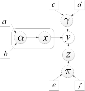
Figure 1: Graphical model for robust Bayesian compressed sensing.

II Hierarchical Prior Model

We develop a Bayesian framework which employs a set of indicator variables $\boldsymbol{z}\triangleq\{z_{m}\}$ to indicate which observation is an outlier, i.e. $z_{m}=1$ indicates that $y_{m}$ is a normal observation, otherwise $y_{m}$ is an outlier. More precisely, we can write

$$y_{m}=\begin{cases}\boldsymbol{a}_{m}^{r}\boldsymbol{x}+w_{m}&z_{m}=1\\ \boldsymbol{a}_{m}^{r}\boldsymbol{x}+w_{m}+e_{m}&z_{m}=0\end{cases}$$ (6)

where $\boldsymbol{a}_{m}^{r}$ denotes the $m$th row of $\boldsymbol{A}$, $e_{m}$ and $w_{m}$ are the $m$th entry of $\boldsymbol{e}$ and $\boldsymbol{w}$, respectively. The probability of the observed data conditional on these indicator variables can be expressed as

$$p(\boldsymbol{y}|\boldsymbol{x},\boldsymbol{z},\gamma)=\prod_{m=1}^{M}(\mathcal{N}(y_{m}|\boldsymbol{a}_{m}^{r}\boldsymbol{x},1/\gamma))^{z_{m}}$$ (7)

in which those “presumed outliers” are automatically disabled when calculating the probability. To infer the indicator variables, a beta-Bernoulli hierarchical prior [11, 12] is placed on $\boldsymbol{z}$, i.e. each component of $\boldsymbol{z}$ is assumed to be drawn from a Bernoulli distribution parameterized by $\pi_{m}$

$$p(z_{m}|\pi_{m})=\text{Bernoulli}(z_{m}|\pi_{m})=\pi_{m}^{z_{m}}(1-\pi_{m})^{1-z_{m}}\quad\forall m$$ (8)

and $\pi_{m}$ follows a beta distribution

$$p(\pi_{m})=\text{Beta}(e,f)\quad\forall m$$ (9)

where $e$ and $f$ are parameters characterizing the beta distribution. Note that the beta-Bernoulli prior assumes the random variables $\{z_{m}\}$ are mutually independent, and so are the random variables $\{\pi_{m}\}$.

To encourage a sparse solution, a Gaussian-inverse Gamma hierarchical prior, which has been widely used in sparse Bayesian learning (e.g. [13, 14, 15, 16]), is employed. Specifically, in the first layer, $\boldsymbol{x}$ is assigned a Gaussian prior distribution

$$p(\boldsymbol{x}|\boldsymbol{\alpha})=\prod_{n=1}^{N}p(x_{n}|\alpha_{n})$$ (10)

where $p(x_{n}|\alpha_{n})=\mathcal{N}(x_{n}|0,\alpha_{n}^{-1})$, and $\boldsymbol{\alpha}\triangleq\{\alpha_{n}\}$ are non-negative hyperparameters controlling the sparsity of the signal $\boldsymbol{x}$. The second layer specifies Gamma distributions as hyperpriors over the precision parameters $\{\alpha_{n}\}$, i.e.

$$p(\boldsymbol{\alpha})=\prod_{n=1}^{N}\text{Gamma}(\alpha_{n}|a,b)=\prod_{n=1}^{N}\Gamma(a)^{-1}b^{a}\alpha_{n}^{a-1}e^{-b\alpha_{n}}$$ (11)

where the parameters $a$ and $b$ are set to small values (e.g. $a=b=10^{-10}$) in order to provide non-informative (over a logarithmic scale) hyperpriors over $\{\alpha_{n}\}$. Also, to estimate the noise variance, we place a Gamma hyperprior over $\gamma$, i.e.

$$p(\gamma)=\text{Gamma}(\gamma|c,d)=\Gamma(c)^{-1}d^{c}\gamma^{c-1}e^{-d\gamma}$$ (12)

where the parameters $c$ and $d$ are set to be small, e.g. $c=d=10^{-10}$. The graphical model of the proposed hierarchical prior is shown in Fig. 1.

III Variational Bayesian Inference

We now proceed to perform Bayesian inference for the proposed hierarchical model. Let $\boldsymbol{\theta}\triangleq\{\boldsymbol{z},\boldsymbol{x},\boldsymbol{\pi},\boldsymbol{\alpha},\gamma\}$ denote the hidden variables in our hierarchical model. Our objective is to find the posterior distribution $p(\boldsymbol{\theta}|\boldsymbol{y})$, which is usually computationally intractable. To circumvent this difficulty, observe that the marginal probability of the observed data can be decomposed into two terms

$$\ln p(\boldsymbol{y})=L(q)+\text{KL}(q||p)$$ (13)

where

$$L(q)=\int q(\boldsymbol{\theta})\ln\frac{p(\boldsymbol{y},\boldsymbol{\theta})}{q(\boldsymbol{\theta})}d\boldsymbol{\theta}$$ (14)

and

$$\text{KL}(q||p)=-\int q(\boldsymbol{\theta})\ln\frac{p(\boldsymbol{\theta}|\boldsymbol{y})}{q(\boldsymbol{\theta})}d\boldsymbol{\theta}$$ (15)

where $q(\boldsymbol{\theta})$ is any probability density function, $\text{KL}(q||p)$ is the Kullback-Leibler divergence between $p(\boldsymbol{\theta}|\boldsymbol{y})$ and $q(\boldsymbol{\theta})$. Since $\text{KL}(q||p)\geq 0$, it follows that $L(q)$ is a rigorous lower bound on $\ln p(\boldsymbol{y})$. Moreover, notice that the left hand side of (13) is independent of $q(\boldsymbol{\theta})$. Therefore maximizing $L(q)$ is equivalent to minimizing $\text{KL}(q||p)$, and thus the posterior distribution $p(\boldsymbol{\theta}|\boldsymbol{y})$ can be approximated by $q(\boldsymbol{\theta})$ through maximizing $L(q)$. Specifically, we could assume some specific parameterized functional form for $q(\boldsymbol{\theta})$ and then maximize $L(q)$ with respect to the parameters of the distribution. A particular form of $q(\boldsymbol{\theta})$ that has been widely used with great success is the factorized form over the component variables in $\boldsymbol{\theta}$ [17]. For our case, the factorized form of $q(\boldsymbol{\theta})$ can be written as

$$q(\boldsymbol{\theta})=q_{z}(\boldsymbol{z})q_{x}(\boldsymbol{x})q_{\alpha}(\boldsymbol{\alpha})q_{\pi}(\boldsymbol{\pi})q_{\gamma}(\gamma)$$ (16)

We can compute the posterior distribution approximation by finding $q(\boldsymbol{\theta})$ of the factorized form that maximizes the lower bound $L(q)$. The maximization can be conducted in an alternating fashion for each latent variable, which leads to [17]

$$\ln q_{x}(\boldsymbol{x})= \langle\ln p(\boldsymbol{y},\boldsymbol{\theta})\rangle_{q_{\alpha}(\boldsymbol{\alpha})q_{\gamma}(\gamma)q_{z}(\boldsymbol{z})q_{\pi}(\boldsymbol{\pi})}+\text{constant}$$

$$\ln q_{\alpha}(\boldsymbol{\alpha})= \langle\ln p(\boldsymbol{y},\boldsymbol{\theta})\rangle_{q_{x}(\boldsymbol{x})q_{\gamma}(\gamma)q_{z}(\boldsymbol{z})q_{\pi}(\boldsymbol{\pi})}+\text{constant}$$

$$\ln q_{\gamma}(\gamma)= \langle\ln p(\boldsymbol{y},\boldsymbol{\theta})\rangle_{q_{x}(\boldsymbol{x})q_{\alpha}(\boldsymbol{\alpha})q_{z}(\boldsymbol{z})q_{\pi}(\boldsymbol{\pi})}+\text{constant}$$

$$\ln q_{z}(\boldsymbol{z})= \langle\ln p(\boldsymbol{y},\boldsymbol{\theta})\rangle_{q_{x}(\boldsymbol{x})q_{\alpha}(\boldsymbol{\alpha})q_{\gamma}(\gamma)q_{\pi}(\boldsymbol{\pi})}+\text{constant}$$

$$\ln q_{\pi}(\boldsymbol{\pi})= \langle\ln p(\boldsymbol{y},\boldsymbol{\theta})\rangle_{q_{x}(\boldsymbol{x})q_{\alpha}(\boldsymbol{\alpha})q_{\gamma}(\gamma)q_{z}(\boldsymbol{z})}+\text{constant}$$

where $\langle\cdot\rangle_{\cdot}$ denotes an expectation with respect to the distributions specified in the subscript. More details of the Bayesian inference are provided below.

1) Update of $q_{x}(\boldsymbol{x})$: We first consider the calculation of $q_{x}(\boldsymbol{x})$. Keeping those terms that are dependent on $\boldsymbol{x}$, we have

$$\ln q_{x}(\boldsymbol{x})\propto \langle\ln p(\boldsymbol{y}|\boldsymbol{x},\boldsymbol{z},\gamma)+\ln p(\boldsymbol{x}|\boldsymbol{\alpha})\rangle_{q_{\alpha}(\boldsymbol{\alpha})q_{\gamma}(\gamma)q_{z}(\boldsymbol{z})}$$

$$\propto -\sum_{m=1}^{M}\frac{\langle\gamma z_{m}(y_{m}-\boldsymbol{a}_{m}^{r}\boldsymbol{x})^{2}\rangle}{2}-\frac{1}{2}\sum_{n}^{N}\langle\alpha_{n}x_{n}^{2}\rangle$$

$$= -\frac{\langle\gamma\rangle(\boldsymbol{y}-\boldsymbol{A}\boldsymbol{x})^{T}\boldsymbol{D}_{z}(\boldsymbol{y}-\boldsymbol{A}\boldsymbol{x})}{2}-\frac{1}{2}\boldsymbol{x}^{T}\boldsymbol{D}_{\alpha}\boldsymbol{x}$$ (18)

where

$$\boldsymbol{D}_{z}\triangleq\text{diag}(\langle{\boldsymbol{z}}\rangle),~{}~{}\boldsymbol{D}_{\alpha}\triangleq\text{diag}(\langle{\boldsymbol{\alpha}}\rangle)$$ (19)

$\langle{\boldsymbol{z}}\rangle$ and $\langle{\boldsymbol{\alpha}}\rangle$ denote the expectation of $\boldsymbol{z}$ and $\boldsymbol{\alpha}$, respectively. It is easy to show that $q(\boldsymbol{x})$ follows a Gaussian distribution with its mean and covariance matrix given respectively by

$$\boldsymbol{\mu}_{x}= \langle\gamma\rangle\boldsymbol{\Phi}_{x}\boldsymbol{A}^{T}\boldsymbol{D}_{z}\boldsymbol{y}$$ (20)

$$\boldsymbol{\Phi}_{x}= \left(\langle\gamma\rangle\boldsymbol{A}^{T}\boldsymbol{D}_{z}\boldsymbol{A}+\boldsymbol{D}_{\alpha}\right)^{-1}$$ (21)

2) Update of $q_{\alpha}(\boldsymbol{\alpha})$: Keeping only the terms that depend on $\boldsymbol{\alpha}$, the variational optimization of $q_{\alpha}(\boldsymbol{\alpha})$ yields

$$\ln q_{\alpha}(\boldsymbol{\alpha})\propto \langle\ln p(\boldsymbol{x}|\boldsymbol{\alpha})+\ln p(\boldsymbol{\alpha}|a,b)\rangle_{q_{x}(\boldsymbol{x})}$$

$$= \sum_{n=1}^{N}(a+0.5)\ln\alpha_{n}-(0.5\left\langle x_{n}^{2}\right\rangle+b)\alpha_{n}$$ (22)

The posterior $q_{\alpha}(\boldsymbol{\alpha})$ therefore follows a Gamma distribution

$$q_{\alpha}(\boldsymbol{\alpha})=\prod_{n=1}^{N}\text{Gamma}(\alpha_{n}|\tilde{a},\tilde{b}_{n})$$ (23)

in which $\tilde{a}$ and $\tilde{b}_{n}$ are given respectively as

$$\tilde{a}= a+0.5$$

$$\tilde{b}_{n}= b+0.5\langle x_{n}^{2}\rangle$$

3). Update of $q_{\gamma}(\gamma)$: The variational approximation of $q_{\gamma}(\gamma)$ can be obtained as:

$$\ln q_{\gamma}(\gamma)\propto \langle\ln p(\boldsymbol{y}|\boldsymbol{x},\boldsymbol{z},\gamma)+\ln p(\gamma|c,d)\rangle_{q_{x}(\boldsymbol{x})q_{z}(\boldsymbol{z})}$$

$$\propto \sum_{m=1}^{M}\left(0.5\langle z_{m}\rangle\ln\gamma-0.5\gamma\langle z_{m}\rangle\langle(y_{m}-\boldsymbol{a}_{m}^{r}\boldsymbol{x})^{2}\rangle\right)$$

$$+(c-1)\ln\gamma-d\gamma$$

$$= (c+0.5\sum_{m=1}^{M}\langle z_{m}\rangle-1)\ln\gamma-(d+0.5\langle(\boldsymbol{y}-\boldsymbol{A}\boldsymbol{x})^{T}$$

$$\boldsymbol{D_{z}}(\boldsymbol{y}-\boldsymbol{A}\boldsymbol{x})\rangle)\gamma$$ (24)

Clearly, the posterior $q_{\gamma}(\gamma)$ obeys a Gamma distribution

$$q_{\gamma}(\gamma)=\text{Gamma}(\gamma|\tilde{c},\tilde{d})$$ (25)

where $\tilde{c}$ and $\tilde{d}$ are given respectively as

$$\tilde{c}= c+0.5\sum_{m=1}^{M}\langle z_{m}\rangle$$ (26)

$$\tilde{d}= d+0.5\langle(\boldsymbol{y}-\boldsymbol{A}\boldsymbol{x})^{T}\boldsymbol{D}_{z}(\boldsymbol{y}-\boldsymbol{A}\boldsymbol{x})\rangle_{q_{x}(\boldsymbol{x})}$$ (27)

in which

$$\langle(\boldsymbol{y}-\boldsymbol{A}\boldsymbol{x})^{T}\boldsymbol{D}_{z}(\boldsymbol{y}-\boldsymbol{A}\boldsymbol{x})\rangle_{q_{x}(\boldsymbol{x})}$$

$$= (\boldsymbol{y}-\boldsymbol{A}\boldsymbol{\mu}_{x})^{T}\boldsymbol{D}_{z}(\boldsymbol{y}-\boldsymbol{A}\boldsymbol{\mu}_{x})+\text{trace}(\boldsymbol{A}^{T}\boldsymbol{D}_{z}\boldsymbol{A}\boldsymbol{\Phi}_{x})$$

4) Update of $q_{z}(\boldsymbol{z})$: The posterior approximation of $q_{z}(\boldsymbol{z})$ yields

$$\ln q_{z}(\boldsymbol{z})\propto \langle\ln p(\boldsymbol{y}|\boldsymbol{x},\boldsymbol{z},\gamma)+\ln p(\boldsymbol{z}|\boldsymbol{\pi})\rangle_{q_{x}(\boldsymbol{x})q_{\gamma}(\gamma)q_{\pi}(\boldsymbol{\pi})}$$

$$\propto \sum_{m=1}^{M}\langle z_{m}\left(-0.5\gamma(y_{m}-\boldsymbol{a}_{m}^{r}\boldsymbol{x})^{2}+\ln\pi_{m}\right)+$$

$$(1-z_{m})\ln(1-\pi_{m})\rangle$$ (28)

Clearly, $z_{m}$ still follows a Bernoulli distribution with its probability given by

$$P(z_{m}=1) =Ce^{\langle\ln\pi_{m}\rangle}e^{-\frac{\gamma\langle(y_{m}-\boldsymbol{a}_{m}^{r}\boldsymbol{x})^{2}\rangle}{2}}$$ (29)

$$P(z_{m}=0) =Ce^{\langle\ln(1-\pi_{m})\rangle}$$ (30)

where $C$ is a normalizing constant such that $P(z_{m}=1)+P(z_{m}=0)=1$, and

$$\langle(y_{m}-\boldsymbol{a}_{m}^{r}\boldsymbol{x})^{2}\rangle= (y_{m}-\boldsymbol{a}_{m}^{r}\boldsymbol{\mu_{x}})^{2}+\boldsymbol{a}_{m}^{r}\boldsymbol{\Phi}_{x}{\boldsymbol{a}_{m}^{r}}^{T}$$

$$\langle\ln\pi_{m}\rangle= \Psi(e+\langle z_{m}\rangle)-\Psi(e+f+1)$$

$$\langle\ln(1-\pi_{m})\rangle= \Psi(1+f-\langle z_{m}\rangle)-\Psi(e+f+1)$$ (31)

The last two equalities can also be found in [12], in which $\Psi(\cdot)$ represents the digamma function.

5) Update of $q_{\pi}(\boldsymbol{\pi})$: The posterior approximation of $q_{\pi}(\boldsymbol{\pi})$ can be calculated as

$$\ln q_{\pi}(\boldsymbol{\pi})\propto \langle\ln p(\boldsymbol{z}|\boldsymbol{\pi})+\ln p(\boldsymbol{\pi}|e,f)\rangle_{q_{z}(\boldsymbol{z})}$$

$$\propto \sum_{m=1}^{M}\langle z_{m}\ln\pi_{m}+(1-z_{m})\ln(1-\pi_{m})+(e-1)\ln\pi_{m}$$

$$+(f-1)\ln(1-\pi_{m})\rangle$$

$$= \sum_{m=1}^{M}\langle(z_{m}+e-1)\ln\pi_{m}+(f-z_{m})\ln(1-\pi_{m})\rangle$$ (32)

It can be easily verified that $q_{\pi}(\boldsymbol{\pi})$ follows a Beta distribution, i.e.

$$q_{\pi}(\boldsymbol{\pi})=\prod_{m}p(\pi_{m})=\prod_{m}\text{Beta}(\langle z_{m}\rangle+e,1+f-\langle z_{m}\rangle)$$ (33)

In summary, the variational Bayesian inference involves updates of the approximate posterior distributions for hidden variables $\boldsymbol{x}$, $\boldsymbol{\alpha}$, $\boldsymbol{z}$, $\boldsymbol{\pi}$, and $\gamma$ in an alternating fashion. Some of the expectations and moments used during the update are summarized as

$$\langle\alpha_{n}\rangle= \frac{\tilde{a}}{\tilde{b}_{n}}$$

$$\langle\gamma\rangle= \frac{\tilde{c}}{\tilde{d}}$$

$$\langle x_{n}^{2}\rangle= \langle x_{n}\rangle^{2}+\boldsymbol{\Phi}_{x}(n,n)$$

$$\langle z_{m}\rangle= \frac{P(z_{m}=1)}{P(z_{m}=1)+P(z_{m}=0)}$$

where $\boldsymbol{\Phi}_{x}(n,n)$ denotes the $n$th diagonal element of $\boldsymbol{\Phi}_{x}$.

IV Simulation Results

We now carry out experiments to illustrate the performance of our proposed method which is referred to as the beta-Bernoulli prior model-based robust Bayesian compressed sensing method (BP-RBCS). As discussed earlier, another robust compressed sensing approach is compensation-based and can be formulated as a conventional compressed sensing problem (5). For comparison, the sparse Bayesian learning method [18, 13] is employed to solve (5), and this method is referred to as the compensation-based robust Bayesian compressed sensing method (C-RBCS). Also, we consider an “ideal” method which assumes the knowledge of the locations of the outliers. The outliers are then removed and the sparse Bayeisan learning method is employed to recover the sparse signal. This ideal method is referred to as RBCS-ideal, and serves as a benchmark for the performance of the BP-RBCS and C-RBCS. Note that both C-RBCS and RBCS-ideal use the sparse Bayesian learning method for sparse signal recovery. The parameters $\{a,b,c,d\}$ of the sparse Bayesian learning method are set to $a=b=c=d=10^{-10}$. Our proposed method involves the parameters $\{a,b,c,d,e,f\}$. The first four are also set to $a=b=c=d=10^{-10}$. The beta-Bernoulli parameters $\{e,f\}$ are set to $e=0.7$ and $f=1-e=0.3$ since we expect that the number of outliers is usually small relative to the total number of measurements. Our simulation results suggest that stable recovery is ensured as long as $e$ is set to a value in the range $[0.5,1]$.

We consider the problem of direction-of-arrival (DOA) estimation where $K$ narrowband far-field sources impinge on a uniform linear array of $M$ sensors from different directions. The received signal can be expressed as

$$\boldsymbol{y}=\boldsymbol{A}\boldsymbol{x}+\boldsymbol{w}$$

where $\boldsymbol{w}$ denotes i.i.d. Gaussian observation noise with zero mean and variance $1/\gamma$, $\boldsymbol{A}\in\mathbb{C}^{M\times N}$ is an overcomplete dictionary constructed by evenly-spaced angular points $\{\theta_{n}\}$, with the $(m,n)$th entry of $\boldsymbol{A}$ given by $a_{m,n}=\exp\left\{-2j\pi(m-1)\sin(\theta_{n})D/\lambda\right\}$, in which $D$ denotes the distance between two adjacent sensors, $\lambda$ represents the wavelength of the source signal, and $\{\theta_{n}\}$ are evenly-spaced grid points in the interval $[-\pi/2,\pi/2]$. The signal $\boldsymbol{x}$ contains $K$ nonzero entries that are independently drawn from a unit circle. Suppose that $T$ out of $M$ measurements are corrupted by outliers. For those corrupted measurements $\{y_{m}\}$, their values are chosen uniformly from $[-10,10]$.

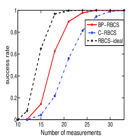
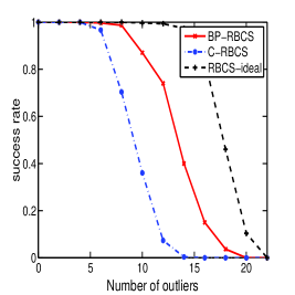
(a)	(b)

Figure 2: (a) Success rates of respective algorithms vs. $M$; (b). Success rates of respective algorithms vs. $T$.

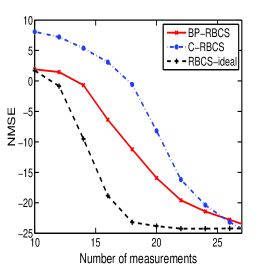
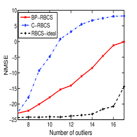
(a)	(b)

Figure 3: (a) NMSEs of respective algorithms vs. $M$; (b). NMSEs of respective algorithms vs. $T$.

We first consider a noiseless case, i.e. $1/\gamma=0$. Fig. 2 depicts the success rates of different methods vs. the number of measurements and the number of outliers, respectively, where we set $N=64$, $K=3$, $T=7$ (the number of outliers) in Fig. 2(a), and $M=25$, $K=3$, $N=64$ in Fig. 2(b). The success rate is computed as the ratio of the number of successful trials to the total number of independent runs. A trial is considered successful if the normalized reconstruction error of the sparse signal $\boldsymbol{x}$ is no greater than $10^{-6}$. From Fig. 2, we see that our proposed BP-RBCS achieves a substantial performance improvement over the C-RBCS. This result corroborates our claim that rejecting outliers is a better strategy than compensating for outliers, particularly when the number of measurements is small, because inaccurate estimation of the compensation vector could lead to a destructive, instead of a constructive, effect on sparse signal recovery. Next, we consider a noisy case with $1/\gamma=0.01$. Fig. 3 plots the normalized mean square errors (NMSEs) of the recovered sparse signal by different methods vs. the number of measurements and the number of outliers, respectively, we set $N=64$, $K=3$, $T=7$ in Fig. 3(a), and $M=25$, $K=3$, $N=64$ in Fig. 3(b). This result, again, demonstrates the superiority of our proposed method over the C-RBCS.

V Conclusions

We proposed a new Bayesian method for robust compressed sensing. The rationale behind the proposed method is to identify the outliers and exclude them from sparse signal recovery. To this objective, a set of indicator variables were employed to indicate which observations are outliers. A beta-Bernoulli prior is assigned to these indicator variables. A variational Bayesian inference method was developed to find the approximate posterior distributions of the latent variables. Simulation results show that our proposed method achieves a substantial performance improvement over the compensation-based robust compressed sensing method.

References

- [1] S. S. Chen, D. L. Donoho, and M. A. Saunders, “Atomic decomposition by basis pursuit,” SIAM J. Sci. Comput., vol. 20, no. 1, pp. 33–61, 1998.
- [2] E. Candés and T. Tao, “Decoding by linear programming,” IEEE Trans. Information Theory, no. 12, pp. 4203–4215, Dec. 2005.
- [3] D. L. Donoho, “Compressive sensing,” IEEE Trans. Inform. Theory, vol. 52, pp. 1289–1306, 2006.
- [4] E. Candes, “The restricted isometry property and its implications for compressive sensing,” Compte Rendus de l’Academie des Sciences, Paris, Serie I, vol. 346, pp. 589–592, 2008.
- [5] M. J. Wainwright, “Information-theoretic limits on sparsity recovery in the high-dimensional and noisy setting,” IEEE Trans. Information Theory, vol. 55, no. 12, pp. 5728–5741, Dec. 2009.
- [6] T. Wimalajeewa and P. K. Varshney, “Performance bounds for sparsity pattern recovery with quantized noisy random projections,” IEEE Journal on Selected Topics in Signal Processing, vol. 6, no. 1, pp. 43–57, Feb. 2012.
- [7] R. G. B. Jason N. Laska, Mark A. Davenport, “Exact signal recovery from sparsely corrupted measurements through the pursuit of justice,” in The 43rd Asilomar Conference on Signals, Systems and Computers, Pacific Grove, California, USA, November 1-4 2009.
- [8] R. C. Kaushik Mitra, Ashok Veeraraghavan, “Analysis of sparse regularization based robust regression approaches,” IEEE Trans. Signal Processing, no. 5, pp. 1249–1257, Mar. 2013.
- [9] R. E. Carrillo, K. E. Barner, and T. C. Aysal, “Robust sampling and reconstruction methods for sparse signals in the presence of impulsive noise,” IEEE Journal of Selected Topics in Signal Processing, no. 2, pp. 392–408, Apr. 2010.
- [10] C. Studer, P. Kuppinger, G. Pope, and H. Bolcskei, “Recovery of sparsely corrupted signals,” IEEE Trans. Information Theory, no. 5, pp. 3115–3130, May 2012.
- [11] L. He and L. Carin, “Exploiting structure in wavelet-based Bayesian compressive sensing,” IEEE Trans. Signal Processing, vol. 57, no. 9, pp. 3488–3497, Sept. 2009.
- [12] J. Paisley and L. Carin, “Nonparametric factor analysis with Beta process priors,” in 26th Annual International Conference on Machine Learning, Montreal, Canada, June 14-18 2009.
- [13] S. Ji, Y. Xue, and L. Carin, “Bayesian compressive sensing,” IEEE Trans. Signal Processing, vol. 56, no. 6, pp. 2346–2356, June 2008.
- [14] Z. Zhang and B. D. Rao, “Extension of SBL algorithms for the recovery of block sparse signals with intra-block correlation,” IEEE Trans. Signal Processing, vol. 61, no. 8, pp. 2009–2015, Apr. 2013.
- [15] Z. Yang, L. Xie, and C. Zhang, “Off-grid direction of arrival estimation using sparse Bayesian inference,” IEEE Trans. Signal Processing, vol. 61, no. 1, pp. 38–42, Jan. 2013.
- [16] J. Fang, Y. Shen, H. Li, and P. Wang, “Pattern-coupled sparse Bayesian learning for recovery of block-sparse signals,” IEEE Trans. Signal Processing, no. 2, pp. 360–372, Jan. 2015.
- [17] D. G. Tzikas, A. C. Likas, and N. P. Galatsanos, “The variational approximation for Bayesian inference,” IEEE Signal Processing Magazine, pp. 131–146, Nov. 2008.
- [18] M. Tipping, “Sparse Bayesian learning and the relevance vector machine,” Journal of Machine Learning Research, vol. 1, pp. 211–244, 2001.