Measuring correlations of cold-atom systems using multiple quantum probes

Abstract

We present a non-destructive method to probe a complex quantum system using multiple impurity atoms as quantum probes. Our protocol provides access to different equilibrium properties of the system by changing its coupling to the probes. In particular, we show that measurements with two probes reveal the system’s non-local two-point density correlations, for probe-system contact interactions. We illustrate our findings with analytic and numerical calculations for the Bose-Hubbard model in the weakly and strongly-interacting regimes, under conditions relevant to ongoing experiments in cold atom systems.

I Introduction

Different phases of matter are fundamentally associated with different correlations among their constituents. These correlations can be encoded in various observables. For example, the ground state of a one-dimensional, single-component Fermi gas has the same density profile as a one-dimensional system of strongly repulsive bosons (Tonks-Girardeau gas), while their momentum distributions are markedly different Cazalilla et al. (2011). This stems from the fact that the momentum distribution contains further information on the two-particle correlations, which also affect other observables such as the excitation spectrum and the structure factor of quantum systems Pines and Nozières (1990); Leggett (2006). While traditionally one could only access these properties via bulk measurements, e.g., neutron scattering off liquid helium, the advent of setups based on cold atoms in optical lattices has opened up new possibilities. For example, the measurement of local two-particle correlations in a one-dimensional gas of bosonic atoms for various interatomic (repulsive) interaction strengths was found Kinoshita et al. (2005) to be in excellent agreement with theoretical calculations Gangardt and Shlyapnikov (2003); Cazalilla (2004); Kheruntsyan et al. (2005). Measurements of the momentum distribution Paredes et al. (2004) and non-local density-density correlation function Fölling et al. (2005) of one-dimensional bosons in a periodic potential have also been performed, and they agree with theoretical findings Paredes et al. (2004); Altman et al. (2004). More recently, $N_{p}$-point non-local correlation functions up to $N_{p}=10$ between two quasi-one-dimensional Bose gases, were measured by matter-wave interferometry Langen et al. (2015). These results underpin the necessity to account for conserved quantities in the description of the non-equilibrium evolution of quantum systems Madroñero et al. (2006); Rigol et al. (2008); Hiller et al. (2012); Birman et al. (2013); Freese et al. (2016).

Common to all these experiments is that they use destructive measurements to study the quantum systems, most frequently the time-of-flight technique, where the trapping potential is switched off and the system allowed to expand before light absorption images are recorded. Based on the development of new measurement and control methods, such as the quantum gas microscope (which enables access to quantum lattice systems with single-site resolution) Bakr et al. (2009); Gemelke et al. (2009); Sherson et al. (2010); Ott (2016); Kuhr (2016), an alternative approach is advancing which considers the use of other quantum objects, such as photons, single atoms or ions as non-destructive quantum probes of many-body quantum systems Ponomarev et al. (2006); Mekhov et al. (2007); Sanders et al. (2010); Zipkes et al. (2010); Schmid et al. (2010); Will et al. (2011); Hunn et al. (2012); Spethmann et al. (2012); Fukuhara et al. (2013); Mayer et al. (2014); Kozlowski et al. (2015).

The idea of using single quantum probes—which often are equipped with the simplest possible internal quantum structure of a qubit—has been implemented to infer diverse properties of the host substrate, from Fröhlich polarons, to work statistics and quantum phase transitions, to the Efimov effect and more Hohmann et al. (2015, 2016); Chin et al. (2010); Dorner et al. (2013); Mazzola et al. (2013); Batalhão et al. (2014); Gessner et al. (2014); Cosco et al. (2015); Johnson et al. (2016); Elliott and Johnson (2016); Levinsen et al. (2015); Haikka et al. (2011). Yet it is clear that a single qubit probe in general cannot suffice to map out the host’s characteristic properties exhaustively, since the probe-system coupling and the thus defined local density of states will generally limit the probe’s diagnostic horizon to a finite subset of the system’s Hilbert space. It is therefore natural to seek a systematic generalization of the quantum probe approach to larger numbers of probes, such as to complement the finite diagnostic power of a single probe, e.g., by directly monitoring spatial correlations.

In the present contribution, we make a first step in this direction by considering two impurities embedded into a host bosonic gas Streif (2016). Specifically, we show that the coherence of a two-probe density matrix enables us to access the two-point correlation function of a strongly-correlated quantum system in a non-destructive way. We start in Sec. II with a general presentation of our two-probe protocol. In Sec. III we study a specific model of bosonic particles in a lattice, the Bose-Hubbard model (BHM), and show that our protocol enables us to determine the average system density as well as the two-point density-density correlation function, both in the superfluid and in the insulating phases of the BHM. Finally, in Sec. IV, we conclude with a summary of our findings and an outlook.

II Two-probe probing protocol

We consider a quantum system, $S$, coupled to two probes, which we label as $L$ (for left) and $R$ (right). The Hamiltonian of the composite system can be written as

$$\hat{H}_{\mathrm{tot}}= \hat{H}_{S}\otimes\mathbb{1}_{L}\otimes\mathbb{1}_{R}+\mathbb{1}_{S}\otimes\hat{H}_{L}\otimes\mathbb{1}_{R}$$

$$+\mathbb{1}_{S}\otimes\mathbb{1}_{L}\otimes\hat{H}_{R}+\hat{H}_{\mathrm{int}}\>,$$ (1)

where $\hat{H}_{S}$ is the Hamiltonian of the system and acts on the Hilbert space $\mathcal{H}_{S}$, $\hat{H}_{\alpha}$ ($\alpha=L,R$) is the Hamiltonian of the left (right) probe acting on its corresponding Hilbert space $\mathcal{H}_{\alpha}$, and $\hat{H}_{\mathrm{int}}$ is the interaction Hamiltonian between the system and the two impurities and therefore acts on $\mathcal{H}_{\mathrm{tot}}=\mathcal{H}_{S}\otimes\mathcal{H}_{L}\otimes\mathcal{H}_{R}$.

We model the probes as two-level systems (qubits), and couple them separately to the system, so that the interaction Hamiltonian reads

$$\hat{H}_{\mathrm{int}} =\hat{V}_{SL}\otimes\bigg{(}g_{L0}\ket{0}_{L}\bra{0}_{L}+g_{L1}\ket{1}_{L}\bra{1}_{L}\bigg{)}\otimes\mathbb{1}_{R}$$

$$+\hat{V}_{SR}\otimes\mathbb{1}_{L}\otimes\bigg{(}g_{R0}\ket{0}_{R}\bra{0}_{R}+g_{R1}\ket{1}_{R}\bra{1}_{R}\bigg{)}.$$ (2)

Here, we have indicated the internal states of each probe qubit by $\ket{0}_{\alpha},\ket{1}_{\alpha}$, respectively, and the parameters $g_{\alpha q}$ describe the interaction between the system and qubit $\alpha=L,R$ when in state $q=\ket{0},\ket{1}$.

Our probing protocol starts with the qubits uncoupled from the system, $g_{\alpha q}(t=0)=0$. The compound initial state reads $\hat{\rho}_{\mathrm{tot}}(t=0)=\hat{\rho}_{S}\otimes\ket{\Phi_{+}}\bra{\Phi_{+}}$, i.e., with the two qubits not entangled with the system, and prepared in the Bell state $\ket{\Phi_{+}}=\left(\ket{00}+\ket{11}\right)/\sqrt{2}$, with the usual notation $\ket{00}=\ket{0}_{L}\otimes\ket{0}_{R}$ and similarly for $\ket{11}$. This entangled state can be prepared from both qubits initially in the ground state $\ket{0}$ and then subjected to a Hadamard gate acting on the left qubit followed by a controlled-NOT gate (with the left qubit as control and the right as target) Nielsen et al. (1998).

At time $t=0$, a unitary non-equilibrium evolution is driven by changing the coupling of one of the internal states of the qubits with the system, e.g., by using a Feshbach resonance. For concreteness, we set $g_{L0}(t)=g_{R0}(t)\equiv g(t)=1$ for $t>0$, while keeping $g_{L1}(t)=g_{R1}(t)=0$. The state of the composite system then evolves under the time evolution operator $\hat{U}(t)=\hat{\mathcal{T}}e^{-\frac{\mathrm{i}}{\hbar}\int_{0}^{t}dt^{\prime}\hat{H}_{\mathrm{tot}}(t^{\prime})}$, where $\hat{\mathcal{T}}$ is the time-ordering operator, so that after a time $t$ the composite system is in the state $\hat{\rho}_{\mathrm{tot}}(t)=\hat{U}(t)\hat{\rho}_{\mathrm{tot}}(0)\hat{U}^{\dagger}(t)$. A trace over the system degrees of freedom yields the reduced density matrix operator of the two qubits, $\hat{\rho}_{\mathrm{Q}}(t)=\mathrm{Tr}_{S}(\hat{\rho}_{\mathrm{tot}}(t))$. We focus our interest on the non-diagonal coherence element, whose time evolution can be expressed as $\braket{11}{\hat{\rho}_{\mathrm{Q}}(t)}{00}=\frac{1}{4}\mathrm{e}^{-\frac{\mathrm{i}}{\hbar}t\Delta}\zeta(t)$. Here, the exponential factor accounts for the free evolution in terms of the energy splitting between the internal states of the two probes, $\Delta=E_{\ket{11}}-E_{\ket{00}}$; without loss of generality, we set this energy difference to zero, i.e. $\Delta=0$. The function $\zeta(t)$ characterizes the coherence element’s time dependence due to the qubits’ coupling to the system; we will refer to it as the coherence function. Note that $\zeta(t)$ will generally depend on the distance between the probes, $\zeta(t)=\zeta(t;\Delta{c})$ (cf. Fig. 1), which we indicate explicitly where necessary.

The moments of the interaction Hamiltonian determine the derivatives of this coherence function (Elliott and Johnson, 2016). For example,

$$\frac{\mathrm{d}\zeta(t)}{dt}\bigg{|}_{t=0} =\frac{\mathrm{i}}{\hbar}\braket{\hat{H}_{\mathrm{int}}}\,,$$ (3)

$$\frac{\mathrm{d^{2}}\zeta(t)}{\mathrm{dt^{2}}}\bigg{|}_{t=0} =-\frac{1}{\hbar^{2}}\braket{\hat{H}_{\mathrm{int}}^{2}}\,,$$ (4)

where the expectation values on the right hand sides are calculated with $\hat{\rho}_{\mathrm{tot}}(t)$. It follows that measurements of $\zeta(t)$ permit us to access several equilibrium expectation values of the system. These expectation values can be related to observables of interest by a suitable choice of the interaction between probes and system. Below, we show that, in particular, for contact probe-system interactions, measurements of the coherence function provide a way to determine the density [Eq. (9)] and the two-point density correlation function [Eq. (10)] of the host substrate.

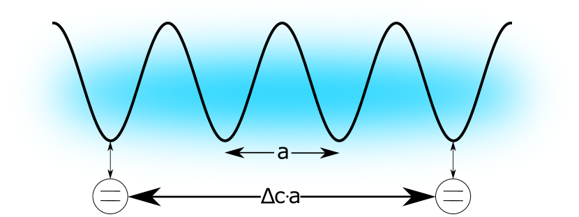
Figure 1: Schematic of a Bose gas (blue shading) in an optical lattice (black line). Two ancillary two-level quantum systems (circles) are coupled to the Bose gas at distinct sites on the lattice, separated by a distance $\Delta{c}$ in units of the lattice constant $a$.

Representing the internal state of each qubit as a spin operator, and using the Pauli spin matrices, $\sigma_{i}$ ($i=x,y,z$), the real and imaginary parts of $\zeta(t)$ can be written

$$\mathrm{Re}(\zeta(t))= \frac{1}{2}\langle\hat{\sigma}_{x}\otimes\hat{\sigma}_{x}-\hat{\sigma}_{y}\otimes\hat{\sigma}_{y}\rangle_{t}$$ (5)

$$\mathrm{Im}(\zeta(t))= \frac{1}{2}\langle\hat{\sigma}_{x}\otimes\hat{\sigma}_{y}+\hat{\sigma}_{y}\otimes\hat{\sigma}_{x}\rangle_{t},$$ (6)

where the bracket $\langle\cdot\rangle_{t}$ represents a trace over $\hat{\rho}_{Q}(t)$. Thus, $\zeta(t)$ can be experimentally determined by measuring the two-qubit correlation functions which enter Eqs. (5) and (6). Alternatively, one can express $\zeta(t)$ in the Bell basis as $\mathrm{Re}(\zeta(t))=2\left(\rho_{Q,++}(t)-\rho_{Q,--}(t)\right)$, $\mathrm{Im}(\zeta(t))=4\,\mathrm{Im}\left(\rho_{Q,+-}(t)\right)$, with $\rho_{Q,++}(t)=\langle\Phi_{+}|\hat{\rho}_{Q}(t)|\Phi_{+}\rangle$ and analogously for $\rho_{Q,--}$ and $\rho_{Q,+-}$, with $\ket{\Phi_{-}}=(\ket{00}-\ket{11})/\sqrt{2}$. It follows that $\zeta(t)$ can also be determined with Bell-state measurements.

III Application to the Bose-Hubbard model

We now apply the protocol described in Sec. II to the case of $N$ cold bosonic atoms loaded into the lowest energy band of an optical lattice with $M$ sites, described by the Bose-Hubbard Hamiltonian Jaksch et al. (1998); Greiner et al. (2002)

$$\hat{H}_{S} =-J\sum_{\braket{i,j}}\hat{a}_{i}^{\dagger}\hat{a}_{j}+\frac{U}{2}\sum_{i=1}^{M}\hat{a}_{i}^{\dagger}\hat{a}_{i}^{\dagger}\hat{a}_{i}\hat{a}_{i}+\mu\sum_{i=1}^{M}\hat{a}_{i}^{\dagger}\hat{a}_{i}\>.$$ (7)

The operator $\hat{a}_{i}^{\dagger}$ ($\hat{a}_{i}$) creates (annihilates) a boson at a lattice site $i=1,\ldots,M$, the index $\braket{i,j}$ indicates summation over nearest neighbor pairs, and the parameters $U$, $J$, and $\mu$ are the on-site interaction energy, the hopping energy and the chemical potential, respectively. We are interested in the translationally invariant system, i.e., in the limit $\{N\to\infty$, $M\to\infty\}$ with fixed average density $n=N/M$.

We now account for both probe impurities by a coupling mediated via a contact density-density interaction potential,

$$\hat{V}_{S\alpha} =\int\mathrm{d}\bm{x}n_{\alpha}(\bm{x})\hat{\Psi}^{\dagger}(\bm{x})\hat{\Psi}(\bm{x})\>, \alpha=L,R$$ (8)

where $\hat{\Psi}(\bm{x})=\sum_{j}w_{j}(\bm{x})\hat{a}_{j}$ is the bosonic field annihilation operator of the system, with $w_{j}(\bm{x})$ the lowest energy Wannier function at lattice site $j=1,\ldots,M$, and $n_{\alpha}(\bm{x})$ the density of qubit $\alpha$ at position $\bm{x}$. Assuming that both impurities are strongly localized at distinct lattice sites ($j_{L}$ and $j_{R}$), we find that they interact with the Wannier function of that very site only. Thus, the interaction term can be written in terms of the boson number operators at these sites, $\hat{V}_{S\alpha}=\eta_{\alpha}\hat{a}_{j_{\alpha}}^{\dagger}\hat{a}_{j_{\alpha}}$, the parameter $\eta_{\alpha}=J\int\mathrm{d}\bm{x}|w_{\alpha}(\bm{x})|^{2}n_{\alpha}(\bm{x})$ being a measure of the interaction strength between the bosons and the qubit at site $j_{\alpha}$. For simplicity, we assume that the local interaction strengths at both probe locations are identical, i.e., $\eta_{L}=\eta_{R}\equiv\eta$.

Substitution of Eq. (8) into Eq. (2), together with Eq. (3), yields the expectation value of the interaction’s contribution to the total Hamiltonian which, due to the specific form of $V_{S\alpha}$, is equal to the bosonic density $\hat{\rho}(j)=\hat{a}^{\dagger}_{j}\hat{a}_{j}$ at site $j$:

$$2\overline{\rho}=\braket{\hat{\rho}(j)+\hat{\rho}(j+\Delta{c})}=\frac{\hbar}{\mathrm{i}\eta}\frac{\mathrm{d}\zeta(t;\Delta{c})}{dt}\bigg{|}_{t=0},$$ (9)

For the first equality, we used that, for translationally invariant systems, $\braket{\hat{\rho}(j)}=\braket{\hat{\rho}(j+\Delta{c})}\equiv\overline{\rho}$, with the integer $\Delta{c}=j_{R}-j_{L}$ the distance between the two qubits in units of the lattice constant $a$ (see Fig. 1). (In an experiment, this can be accomplished by trapping the two qubits in a separate optical lattice formed by crossing two laser beams; the inter-qubit distance $\Delta{c}$ can then be precisely tuned by changing the angle between the propagation directions of the beams; see, e.g., (Huckans et al., 2009).)

Similarly, using Eq. (4), we find the bosonic density-density correlation function $\mathrm{Cor}(\Delta{c})=\braket{\hat{\rho}(j)\hat{\rho}(j+\Delta{c})}$ in terms of the qubits’ coherence function:

$$\braket{\left[\hat{\rho}(j)+\hat{\rho}(j+\Delta{c})\right]^{2}}=-\frac{\hbar^{2}}{\eta^{2}}\frac{\mathrm{d}^{2}\zeta(t;\Delta{c})}{dt^{2}}\bigg{|}_{t=0}\>.$$ (10)

Again, given the system’s translational invariance, $\braket{\hat{\rho}(j)^{2}}=\braket{\hat{\rho}(j+\Delta{c})^{2}}$, the last expression can be rewritten as

$$\mathrm{Cor}(\Delta{c}) =\frac{\hbar^{2}}{2\eta^{2}}\frac{\mathrm{d^{2}}}{dt^{2}}\bigg{[}\frac{1}{2}\zeta(t;\Delta c=0)-\zeta(t;\Delta c)\bigg{]}\bigg{|}_{t=0}.$$ (11)

This result implies that measurements of the qubits’ coherence function $\zeta(t)$ provide access to the system’s density-density correlation function. We remark that this result depends on the qubits-system coupling, Eq. (8), but not on the specific form of the system Hamiltonian $\hat{H}_{S}$ beyond its translational invariance. In the following sections, we assess the experimental feasibility of our protocol by simulating the outcome of the protocol in both the superfluid ($U/J\ll 1$) and the insulating ($U/J\gg 1$) phases of the one-dimensional Bose-Hubbard model, and comparing them with exact results for $\mathrm{Cor}(\Delta c)$ in both limits.

III.1 Weak interactions: Superfluid phase

In the regime of weak interactions ($U/J\ll 1$), we can use Bogoliubov theory (Pitaevskii and Stringari, 2003) to calculate both the coherence function $\zeta(t)$ and the density-density correlation function $\mathrm{Cor}(\Delta{c})$ analytically (see also Mayer et al. (2014) and Mayer et al. (2015)). We start from the Bose-Hubbard Hamiltonian, Eq. (7), for a one-dimensional system of homogeneous density $n$. We first transform the annihilation operators from the site basis, $\hat{a}_{i}$, to the momentum basis, $\hat{b}_{k}=(M)^{-1/2}\sum_{j}\hat{a}_{j}e^{\mathrm{i}kaj}$, and similarly for the creation operator $\hat{b}_{k}^{\dagger}$. A Bogoliubov transformation to quasiparticle operators, $\hat{d}_{k}=u_{k}\hat{b}_{k}+v_{k}\hat{b}_{-k}^{\dagger}$, brings the system Hamiltonian into the diagonal form $\hat{H}_{S}=\sum_{k}\hbar\omega_{k}\hat{d}_{k}^{\dagger}\hat{d}_{k}$, with $\hat{d}_{k}$ ($\hat{d}_{k}^{\dagger}$) the annihilation (creation) operator of Bogoliubov quasiparticles of quasi-momentum $k$, and $\omega_{k}=\sqrt{\epsilon_{k}(\epsilon_{k}+2U\overline{\rho})}$ the quasiparticle dispersion relation in terms of the single-particle energies $\epsilon_{k}=2J(1-\cos{(ka)})$, with $a$ the lattice constant and $\overline{\rho}$ the bosonic density (Lewenstein et al., 2012).

With this transformation, we rewrite the density matrix of the lattice bosons by expressing the bosonic operators in terms of Bogoliubov quasiparticle operators

$$\hat{\rho}_{j} =\hat{a}^{\dagger}_{j}\hat{a}_{j}=\frac{1}{M}\sum_{k,k^{\prime}}\hat{b}_{k}^{\dagger}\hat{b}_{k^{\prime}}e^{\mathrm{i}kaj}e^{-\mathrm{i}k^{\prime}aj}$$

$$=\overline{\rho}+\frac{\sqrt{N_{0}}}{M}\sum_{k}\sqrt{\frac{\epsilon_{k}}{\omega_{k}}}\left(d_{k}^{\dagger}e^{\mathrm{i}kaj}+d_{k}e^{-\mathrm{i}kaj}\right).$$ (12)

In the second line, we have applied Bogoliubov’s approximation, i.e., we assume that the occupation of $k\neq 0$ modes is small [$(N-N_{0})/N\ll 1$], and neglect terms of quadratic (or higher) order in quasiparticle operators (Pitaevskii and Stringari, 2003; Lewenstein et al., 2012). By inserting Eq. (12) into the definition of the two-point density correlation function, we reach the following analytic expression valid in the weakly-interacting limit

$$\mathrm{Cor}(\Delta{c}) =\overline{\rho}^{2}+\frac{\overline{\rho}}{M}\sum_{k}\frac{\epsilon_{k}}{\omega_{k}}(2n^{\mathrm{th}}_{k}+1)\cos{(ka\Delta{c})}\>,$$ (13)

where we have evaluated the occupations of the Bogoliubov modes in a thermal state, $\braket{\hat{d}_{k}^{\dagger}\hat{d}_{k}}=n^{\mathrm{th}}_{k}=1/(e^{\beta\hbar\omega_{k}}-1)$, with $\beta$ the inverse temperature, and we have dropped the anomalous averages $\braket{\hat{d}_{k}\hat{d}_{-k}}$, as they are negligible at the low temperatures where the Bogoliubov approximation applies Griffin (1996). At zero temperature ($\beta\to\infty$), Eq. (13) satisfies the sum rule established in Ref. Damski and Zakrzewski (2015) for density-density correlations in the ground state, which re-expresses the sum rule relating the dynamic structure factor to the static structure factor, which in turn is sensitive to two-body interactions in bosonic lattice systems Menotti et al. (2003).

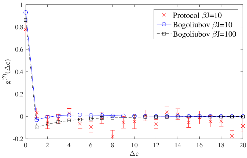
Figure 2: Weak interactions. Normalized correlation function obtained with Eq. (11) simulating $N_{\mathrm{exp}}=10^{4}$ experiments (crosses), compared with the analytic results Eq. (13) (lines with symbols), for a system initially at equilibrium at inverse temperature $\beta J=10$ and $\beta J=100$. Other parameters used are $\eta=0.4J$ and $U/J=0.1$.

Based on Eq. (13), we plot in Fig. 2 the normalized second-order correlation function,

$$g^{(2)}(\Delta{c})=\frac{\braket{\hat{\rho}(0)\hat{\rho}(\Delta{c})}-\braket{\hat{\rho}(0)}\braket{\hat{\rho}(\Delta{c})}}{\braket{\hat{\rho}(0)}^{2}},$$ (14)

as a function of the inter-probe distance $\Delta{c}$ for different temperatures. We see that, for all temperatures, the correlation vanishes for distances beyond a few lattice sites, which agrees with the picture that, in the non-interacting limit, the system is effectively described by a product of on-site coherent states so that $\braket{\hat{\rho}(0)\hat{\rho}(\Delta{c})}=\braket{\hat{\rho}(0)}\braket{\hat{\rho}(\Delta{c})}$ Bloch et al. (2008). Weakly-interacting homogeneous one-dimensional Bose gases also converge to this limit fairly quickly Deuar et al. (2009).

We proceed now to compare these analytic calculations with the estimation by means of the coherence function $\zeta(t)$. To evaluate the right-hand side of Eq. (11), we rewrite the system-qubit interaction Hamiltonian in terms of Bogoliubov operators,

$$\hat{V}=\hat{V}_{SL}+\hat{V}_{SR}=2\overline{\rho}\eta+\sum_{k}\left(\eta_{k}^{\star}\hat{d}_{k}^{\dagger}+\eta_{k}\hat{d}_{k}\right),$$ (15)

where $\eta_{k}=\eta\sqrt{n\epsilon_{k}/M\omega_{k}}(e^{-\mathrm{i}kaj_{L}}+e^{-\mathrm{i}kaj_{R}})$ is the coupling strength of the qubits with the Bogoliubov mode of quasi-momentum $k$. Substituting these expressions into $\hat{H}_{\mathrm{int}}$ allows us to calculate analytically the time evolution of the composite system and, therefore, to determine the coherence function $\zeta(t)$. Full details of the derivation are reported in Appendix A (see also Streif (2016)); here we quote only the final result,

$$\zeta(t) =e^{2\mathrm{i}\eta\overline{\rho}t}\exp\left[-\mathrm{i}\sum_{k}\frac{|\eta_{k}|^{2}}{\omega_{k}^{2}}[\omega_{k}t-\sin(\omega_{k}t)]\right]$$

$$\times\exp{\left[\sum_{k}\left(-2\frac{|\eta_{k}|^{2}}{\omega_{k}^{2}}\sin^{2}\frac{\omega_{k}t}{2}\coth\frac{\beta\omega_{k}}{2}\right)\right]}\>.$$ (16)

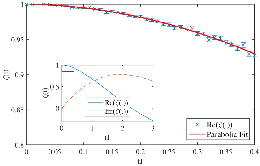
Figure 3: Real part of the coherence function with added Gaussian noise (symbols) and a parabolic fit (solid line). Inset: Real (solid blue line) and imaginary (dashed red line) parts of $\zeta(t)$, Eq. (16), for the case $\Delta{c}=5$. Here, we used a system with $M=1000$ lattice sites and $N=1000$ bosons; and, therefore, an average density $\overline{\rho}=1$. The system is initially in a thermal state with $\beta J=10$; other parameters as in Fig. 2.

In an experiment, the coherence function $\zeta(t)$ can only be measured at discrete times, $t_{r}$. In addition, for each time $t_{r}$, the expectation value defining $\zeta(t_{r})$ is obtained upon accumulation of repeated measurements of the qubits’ state, with individual measurement outcomes exhibiting quantum (shot) noise. To simulate this unavoidable spread of experimental measurement events, and to estimate how many measurements one would need for their statistical average to converge to the expectation value, we follow the scheme in Ref. Johnson et al. (2016) and add Gaussian noise to the calculated values of $\zeta(t_{r})$; see Appendix B for details on how to determine the corresponding variance. As one would do in an experiment, to reduce the ensuing uncertainty in $\zeta(t_{r})$, we repeat the simulated experiment a number $N_{\mathrm{exp}}$ of times and average over all outcomes, for each inter-probe distance $\Delta{c}$. The values of $\zeta(t_{r})$ estimated in this way are presented in Fig. 3 for a system with average density $\overline{\rho}=1$. Here, one can note that the real part of $\zeta(t)$ has a parabolic dependence on time, while the imaginary part is linear around $t=0$. It follows that the second derivative will be real, in accordance with our expectations for the density-density correlation function [cf. Eq. (11)]. Thus, in practice it suffices to measure only the real part of $\zeta(t)$, Eq. (5).

Given the smooth character of $\zeta(t_{r})$, we fit a quadratic polynomial through these values, which enables us to calculate the right-hand side of Eq. (11) and determine the two-point correlation function. We show the corresponding results for $\beta J=10$ in Fig. 2, which are in fair agreement with the analytic result (13). In particular, we see that the value of $g^{(2)}(0)$ derived from the protocol shows the characteristic enhancement of the superfluid phase. Reducing the statistical uncertainty of $g^{(2)}(\Delta{c})$ for $\Delta{c}\gg 1$ requires a relatively large number of measurements $N_{\mathrm{exp}}$, in line with previous experimental determinations of $g^{(2)}(\Delta{c})$ in cold atomic setups Öttl et al. (2005); Schellekens et al. (2005). In the framework of the present two-probe protocol, these fluctuations, and correspondingly $N_{\mathrm{exp}}$, can be reduced by running in parallel an arrangement with $N_{\mathrm{pairs}}$ pairs of probes in a double-well superlattice (Anderlini et al., 2007; Fölling et al., 2007; Hofferberth et al., 2007; Hangleiter et al., 2015); a setup with $N_{\mathrm{pairs}}=100$ probe pairs would reach the precision shown in Fig. 2 with only 100 measurement runs.

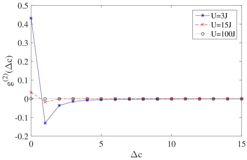
Figure 4: Correlation function $g^{(2)}(\Delta{c})$ for the ground state in the strongly-interacting regime for different interactions strengths, $U/J=3$, $15$, and $100$, as indicated. These points represent the numerically exact expectation values of number operator pairs, $\left(\braket{\hat{\rho}_{i}\hat{\rho}_{j}}-\braket{\hat{\rho}_{i}}\braket{\hat{\rho}_{j}}\right)/\braket{\hat{\rho}_{i}}^{2}$, from the TNT calculation.

III.2 Strong interactions: Insulating phase

For stronger interactions $U/J\gtrsim 1$, the correlations between the bosons in the lattice invalidate an approach based on the Bogoliubov treatment. An efficient method to deal with this situation is Tensor Network Theory (TNT), which provides numerically exact ground state properties of strongly-correlated systems, in particular, of the one-dimensional BHM Orús (2014); Al-Assam et al. (2016a). Here, we apply this method to calculate $g^{(2)}(\Delta{c})$ in the ground state of this model using the implementation Oxford TNT library Al-Assam et al. (2016b). As we are interested in investigating non-local correlation functions, we choose a large system with $M=101$ lattice sites, and $\overline{\rho}=1$ as before, and calculate $g^{(2)}(\Delta{c})$ around the central lattice site so that boundary effects are negligible and the system can still be considered (approximately) translationally invariant. For the calculations presented below, we have checked that sufficient accuracy is reached bounding the site occupation to a maximum of four bosons per site and fixing a truncation parameter (maximum number of Schmidt coefficients) of $\chi=100$.

The TNT method allows us to calculate directly the expectation values of the number operator at each lattice site, $\braket{\hat{\rho}_{i}}$, and all pairs of number operators, $\braket{\hat{\rho}_{i}\hat{\rho}_{j}}$. From these, we obtain directly the normalized two-point correlation function $g^{(2)}(\Delta{c})=\left(\braket{\hat{\rho}_{i}\hat{\rho}_{i+\Delta{c}}}-\braket{\hat{\rho}_{i}}\braket{\hat{\rho}_{i+\Delta{c}}}\right)/\braket{\hat{\rho}_{i}}^{2}$; the results for increasing values of $U/J$ are shown in Fig. 4. As expected, in the limit $U/J\rightarrow\infty$ we recover that $g^{(2)}(\Delta{c})=0$ $\forall\Delta{c}$ as the ground state is a product of on-site Fock states with no density fluctuations Bloch et al. (2008); Endres et al. (2013). These results constitute the test-bed corresponding to the left-hand site of Eq. (11), which we will compare to the outcome of the protocol to obtain $\zeta(t)$ and its derivatives.

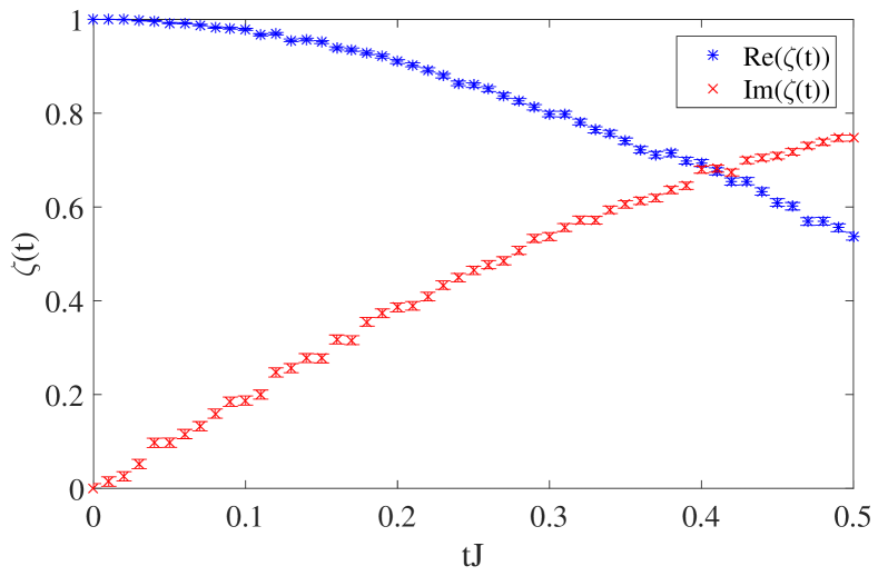
(a)  (b) 

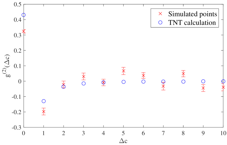
Figure 5: Strong interactions. (a) Real (asterisks) and imaginary (crosses) parts of the coherence function $\zeta(t)$ for $U/J=3$. Other parameters are $\Delta{c}=5$, $M=101$, $\overline{\rho}=1$, and $\eta=J$. (b) Normalized correlation function $g^{(2)}(\Delta{c})$ for the same parameters. The results of the measurement protocol with $N_{\mathrm{exp}}=10^{4}$ (crosses) agree with the numerically exact values calculated with the TNT method (circles).

We calculate $\zeta(t)$ in the strongly-interacting regime in the following way: The coherence function can be written as a trace over system operators only, $\zeta(t)=\mathrm{Tr}_{S}(\hat{U}_{1}(t)\hat{U}_{0}(t)\hat{\rho}_{\beta})$ [cf. Eq. (17)]. Here, $\hat{U}_{0}(t)$ is the evolution operator over a time $t$ with the initial system Hamiltonian, while $\hat{U}_{1}(t)$ is the evolution operator including the coupling to the qubits. For probe qubits localized at lattice sites and coupled to the bosons by contact interactions of strength $\eta$, the effect of the probe-boson coupling amounts to a local shift of the bosons’ chemical potential, $\mu\to\mu-\eta$, at the sites where the probes are located. Thus, we can obtain $\zeta(t_{r})$ at different time steps $t_{r}$ by calculating the expectation value $\mathrm{Tr}_{S}(\hat{U}_{1}(t)\hat{U}_{0}(t)\hat{\rho}_{\beta})$ with $\hat{\rho}_{\beta}$ the ground state of the bosonic system in a lattice with modified local potential at the probe sites.

In our numerical calculations, we take $t_{r}=r\Delta{t}$ with $\Delta{t}=\hbar\times 0.01/J$ and $r=0,\ldots,20$. As for the weakly-interacting regime, we simulate the uncertainty in an experiment by adding noise to each simulated data point, $\zeta(t_{r})$, and calculate the numerical second derivative at $t=0$. We repeat this procedure for all integer distances between the two qubits $0\leq\Delta{c}\leq 15$ ($\ll M$ to avoid boundary effects). The coherence function, $\zeta(t)$ obtained in this way is shown in Fig. 5(a). We observe that both real and imaginary parts exhibit broadly a behavior similar to that of the weakly interacting system. However, the correlation function that one obtains from this according to Eq. (11) is notably different, as shown in Fig. 5(b), where we compare the value of $g^{(2)}(\Delta{c})$ obtained from the coherence function by using Eq. (11) with the numerically exact values derived from the TNT ground state (the latter values are the same as those in Fig. 4 for $U/J=3$). We see that there is a good agreement between the two calculations, as happened in the weakly interacting regime. In particular, the estimation of the correlation function using our protocol is able to detect the reduction in $g^{(2)}(0)$ as the system gets deeper into the Mott insulating phase, $U/J\gg 1$. To illustrate this point, we show in Fig. 6 the normalized correlation function $g^{(2)}(\Delta{c})$ at selected distances $\Delta{c}$ for different values of $U/J$ across the Mott insulator–to–superfluid transition. First, we observe that the outcome of our protocol in each case is very close to the exact result (calculated with Bogoliubov theory for weak interactions and with TNT for stronger interactions). Physically, the local correlation, $g^{(2)}(0)$, decreases steadily as the repulsion between bosons increases, and it vanishes in the limit $U/J\gg 1$. Correlations at larger distances are negative (meaning, it is less probable to find a particle at distance $\Delta{c}$ in the actual ground state than what one would predict by relying only on the average density) and generally of smaller magnitude than the local correlation; they also vanish in the strongly repulsive limit, as expected for a Mott insulator.

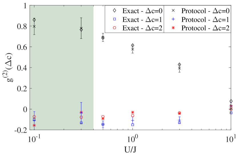
Figure 6: Correlation function $g^{(2)}(\Delta{c})$ for $\Delta{c}\in\{0,1,2\}$ and different values of $U/J$. Bogoliubov theory was used for $U/J\leq 0.4$ with a $\beta J=1000$ thermal state (shaded region), and TNT for larger values of $U/J$. For clarity, we do not include error bars for the $\Delta{c}=2$ calculation; they are similar to those for $\Delta{c}=1$.

IV Discussion and Outlook

In this paper, we have developed a framework to study correlation functions in cold atom systems by using multiple atomic impurities as quantum probes, a setup realized in recent experiments where potassium Ospelkaus et al. (2006); Will et al. (2011); Catani et al. (2012) or cesium Spethmann et al. (2012); Hohmann et al. (2016) atomic impurities were immersed in larger rubidium Bose gases.

We have presented a protocol which is able to measure the density-density correlations of the system relying on measuring the internal states of two probes and studying an off-diagonal element of their reduced density matrix. We have shown that the results of this protocol agree with those of analytic and numerically exact calculations for a one-dimensional Bose-Hubbard model in both the weakly and the strongly interacting regimes. In particular, we have shown that the protocol is able to witness the change in correlations across the superfluid–to–Mott insulator transition.

Non-local density correlations in quantum gases have previously been measured by various methods, including noise interferometry, Bragg spectroscopy, and matter-wave interferometry. Let us briefly contrast our proposal with these techniques. In Bragg spectroscopy, some of the atoms in the system are excited by two-photon Bragg scattering into a state of given momentum and energy. This provides access to the dynamic structure factor of the gas, which is the Fourier transform of the density correlation function Kozuma et al. (1999); Stenger et al. (1999); Menotti et al. (2003); Rey et al. (2005). This method inevitably destroys the initial quantum state of the system, in contrast to our proposal, which is inherently non-destructive and, thus, could permit a time-dependent monitoring of the evolution of correlations. In addition, our protocol can be extended to using $N>2$ quantum probes to determine $N$-point correlation functions.

Matter-wave interferometry Cronin et al. (2009) is a destructive measurement method especially suited to probing the phase structure of bosonic quantum gases. As mentioned earlier, it has been used recently to measure density correlation functions up to $10^{\mathrm{th}}$ order between two quasi-one-dimensional bosonic gases Langen et al. (2015). However, the application of this method to higher-dimensional systems would require a rather involved analysis of the corresponding multi-dimensional phase interference pattern. In contrast, it is straightforward to see that our protocol applies to systems of any dimensionality.

Noise interferometry retrieves information on particle correlations in atomic gases by analyzing the shot-to-shot fluctuations in absorption images of the system after time-of-flight evolution Altman et al. (2004); Greiner et al. (2005); Fölling et al. (2005). In strongly correlated phases, where the time-of-flight technique is not suitable, one could implement noise interferometry by imaging the atoms with a quantum gas microscope Bakr et al. (2009); Gemelke et al. (2009); Sherson et al. (2010); Ott (2016); Kuhr (2016); Cheuk et al. (2015); Haller et al. (2015); Miranda et al. (2015); Edge et al. (2015); Cocchi et al. (2016); Boll et al. (2016); Parsons et al. (2016); Drewes et al. (2016) to analyze correlations in optical lattice setups. Our proposal constitutes a complementary approach of similar experimental complexity, particularly suited to multicomponent setups with impurities Ospelkaus et al. (2006); Will et al. (2011); Catani et al. (2012); Spethmann et al. (2012); Hohmann et al. (2016), with the distinctive feature of allowing non-destructive measurements.

The main challenge of our proposal may lie in the dynamical control of the probe-system coupling. Manipulation via Feshbach resonances is an option if these are available between the atomic species involved. More generally, one could envisage probing a one- or two-dimensional gas by allowing the impurities to “fall through” it, pulled by gravity or driven by an external field. This would turn on and off the interactions without changing the state of the system appreciably (given that there are many more atoms in the background than impurities). This approach could be implemented exploiting existing experimental schemes in which the impurities are trapped near but outside the system and then driven into it for a fixed amount of time Spethmann et al. (2012); Hohmann et al. (2016), or made to penetrate it periodically Eto et al. (2016).

In summary, the framework presented here opens up new possibilities for the experimental investigation of quantum many-body systems and, especially, systems of cold atoms in optical lattices. The protocol can be extended in various ways, e.g., to estimate $N$-point correlation functions. Another possibility stems from the freedom of choosing the kind of interaction Hamiltonian between qubits and system, different choices allowing one to gain access to different observables. For example, by using Raman transitions (Recati et al., 2005), the evolution of the probes becomes sensitive to the phase of the matter wave and one could measure cross-correlation functions (Kaminishi et al., 2015).

Appendix A Bogoliubov treatment of the weakly interacting system

We briefly expand on the explicit calculation of the coherence function $\zeta(t)$ for weak interactions, with the help of Bogoliubov theory, and following the procedure outlined in Johnson et al. (2016). The first step is to introduce a set of projection operators on the Hilbert space of the two qubits,

$$\begin{array}[]{ll}\hat{\mathcal{P}}_{11}=\ket{11}\bra{11}\,,&~{}~{}~{}\hat{\mathcal{P}}_{10}=\ket{10}\bra{10}\,,\\ \hat{\mathcal{P}}_{01}=\ket{01}\bra{01}\,,&~{}~{}~{}\hat{\mathcal{P}}_{00}=\ket{00}\bra{00}\,.\end{array}$$

This enables us to rewrite the full Hamiltonian in a more convenient form.

$$\hat{H}_{\mathrm{tot}} =\hat{\mathcal{P}}_{11}\otimes\left(E_{1}+\hat{H}_{S}+g_{L1}\hat{V}_{SL}+g_{R1}\hat{V}_{SR}\right)+$$

$$+\hat{\mathcal{P}}_{10}\otimes\left(E_{2}+\hat{H}_{S}+g_{L1}\hat{V}_{SL}+g_{R0}\hat{V}_{SR}\right)+$$

$$+\hat{\mathcal{P}}_{01}\otimes\left(E_{3}+\hat{H}_{S}+g_{L0}\hat{V}_{SL}+g_{R1}\hat{V}_{SR}\right)+$$

$$+\hat{\mathcal{P}}_{00}\otimes\left(E_{4}+\hat{H}_{S}+g_{L0}\hat{V}_{SL}+g_{R0}\hat{V}_{SR}\right)\,$$

As stated in the text, we are interested in the time evolution of the qubits only. Therefore, after calculating the time evolution of the composite system, we trace out the degrees of freedom of the bosons. After that, we concentrate on the coherence element of the two-qubit density matrix, $\braket{11}{\hat{\rho}_{\mathrm{Q}}}{00}$. We find that the coherence function can be determined by calculating the expectation value

$$\zeta(t)=\mathrm{Tr}_{S}(\hat{U}_{1}(t)\hat{U}_{0}(t)\hat{\rho}_{S})$$ (17)

with the initial state of the system $\hat{\rho}_{S}$. In this expression

$$\hat{U}_{0}(t)=\hat{\mathcal{T}}\exp{\left(-\frac{\mathrm{i}}{\hbar}\int_{0}^{t}\mathrm{dt^{\prime}}\hat{H}_{S}\right)}$$

is the time evolution operator with the unperturbed system Hamiltonian, and

$$\hat{U}_{1}(t)=\hat{\mathcal{T}}\exp{\left(-\frac{\mathrm{i}}{\hbar}\int_{0}^{t}\mathrm{dt^{\prime}}(\hat{H}_{S}+g(\hat{V}_{SL}+\hat{V}_{SR}))\right)}$$

is the time evolution operator with the Hamiltonian including the coupling to the probes, where we have used that $g_{L0}=g_{R0}=1$ and $g_{L1}=g_{R1}=0$. It is worth noting the similarity of $\zeta(t)$ to the Loschmidt echo (Peres, 1984; Jalabert and Pastawski, 2001), which is a function that enables us to characterize memory effects in the dynamics of quantum systems (see, e.g., Haikka et al. (2012)).

For simplicity, we change into the interaction picture, where $\hat{U}_{0}=\mathbb{1}$. The remaining time evolution operator simplifies to a more convenient expression:

$$\hat{U}_{1}(t)=\hat{\mathcal{T}}\exp{\left(-\frac{\mathrm{i}}{\hbar}\int_{0}^{t}dt^{\prime}\hat{V}_{\mathrm{int}}(t^{\prime})\right)}\>.$$

Here, $\hat{V}_{\mathrm{int}}(t)$ is the interaction part of the Hamiltonian in the interaction picture,

$$\hat{V}_{\mathrm{int}}(t)=2\overline{\rho}\eta+\sum_{k}\left(\eta_{k}^{\star}e^{\mathrm{i}\omega_{k}t}\hat{b}_{k}^{\dagger}+\eta_{k}\hat{b}_{k}e^{-\mathrm{i}\omega_{k}t}\right)\>.$$

We can simplify the expression for $\hat{U}_{1}$ by applying the Magnus expansion Dattoli et al. (1986). To this end, we introduce an operator $\hat{A}$ by

$$\hat{\mathcal{T}}\exp{\left(-\frac{\mathrm{i}}{\hbar}\int_{0}^{t}dt^{\prime}\hat{V}_{\mathrm{int}}(t^{\prime})\right)}=\mathrm{e}^{\hat{A}}\>.$$

This operator can be expressed as a sum of operators $\hat{A}=\sum_{i}\hat{A}_{i}$ which are related to commutators of the interaction Hamiltonian:

$$\hat{A}_{1} =-\mathrm{i}\int_{0}^{t}dt^{\prime}\hat{V}_{\mathrm{int}}(t^{\prime})$$

$$\hat{A}_{2} =\frac{1}{2}\int_{0}^{t}\mathrm{dt^{\prime}}\int_{0}^{t^{\prime}}\mathrm{dt^{\prime\prime}}[\hat{V}_{\mathrm{int}}(t^{\prime}),\hat{V}_{\mathrm{int}}(t^{\prime\prime})]$$

$$\vdots.$$

Given the form of $\hat{V}_{\mathrm{int}}$ above, the commutators at different times are c-numbers, $[\hat{V}_{\mathrm{int}}(t^{\prime}),\hat{V}_{\mathrm{int}}(t^{\prime\prime})]=-2i\sum_{k}|\eta_{k}|^{2}\sin{(\omega_{k}(t^{\prime}-t^{\prime\prime}))}$. Therefore, all terms of the expansion beyond the second term vanish. Thus, we can write the coherence function as

$$\zeta(t) =e^{2\mathrm{i}\overline{\rho}\eta t}\exp{\left[-\mathrm{i}\sum_{k}\frac{|\eta_{k}|^{2}}{\omega_{k}^{2}}[\omega_{k}t-\sin{(\omega_{k}t)}]\right]}$$

$$\times\mathrm{Tr}\left[\exp\left\{-\mathrm{i}\sum_{k}\left(\gamma_{k}\hat{d}_{k}^{\dagger}+\gamma_{k}^{\star}\hat{d}_{k}\right)\right\}\hat{\rho}_{S}\right]$$ (18)

where we have defined $\gamma_{k}=\frac{\eta_{k}^{\star}}{\omega_{k}}\left(\frac{e^{i\omega_{k}t}-1}{\mathrm{i}}\right)$. We are left with the task of calculating the trace over the initial state $\hat{\rho}_{S}$. A close investigation of this expression reveals that the operator acting on $\hat{\rho}_{S}$ is a displacement operator, $\hat{\mathcal{D}}(\alpha)=e^{\alpha\hat{d}^{\dagger}-\alpha^{\star}\hat{d}}$, for each Bogoliubov mode with corresponding displacement $\mathrm{i}\gamma_{k}$. Due to this and the commutation relations of Bogoliubov operators, $[\hat{d}_{k}^{\dagger},\hat{d}_{k^{\prime}}]=\delta_{k,k^{\prime}}$, we can write the trace in the last line of Eq. (18) as the expectation value of a product of displacement operators

$$\mathrm{trace} =\mathrm{Tr}\left[\prod_{k}\hat{\mathcal{D}}_{k}(\mathrm{i}\gamma_{k})\hat{\rho}_{\beta}\right]$$

$$=\sum_{\{n_{k}\}}\prod_{k}\frac{\braket{\hat{\rho}_{k}}^{n_{k}}}{(1+\braket{\hat{\rho}_{k}})^{n_{k}+1}}\braket{\{n_{k}\}}{\prod_{k^{\prime}}\hat{\mathcal{D}}_{k^{\prime}}(\mathrm{i}\gamma_{k^{\prime}})}{\{n_{k}\}}.$$

Here, we have considered that initially the system is in a thermal equilibrium state at inverse temperature $\beta$, so that $\hat{\rho}_{S}=\exp(-\beta\hat{H}_{S})/Z$, with the partition function $Z=\mathrm{Tr}[\exp(-\beta\hat{H}_{S})]$, and then used the diagonal representation of the thermal state in the Fock basis.

The action of a displacement operator on a Fock state $\ket{n}$ is to generate a displaced Fock state $\ket{n,\gamma}$. The remaining overlap of two of these states can be expressed by (Wunsche, 1991)

$$\braket{n,\gamma}{m,\alpha}$$

$$=\braket{\gamma}{\alpha}\sqrt{\frac{n!}{m!}}(\gamma^{\star}-\alpha^{\star})^{m-n}L_{n}^{m-n}[(\gamma-\alpha)(\gamma^{\star}-\alpha^{\star})]\>,$$

where $L_{n}^{a}(x)$ are the generalized Laguerre polynomials and $\braket{\gamma}{\alpha}=\exp[-\frac{1}{2}\left(|\gamma|^{2}+|\alpha|^{2}-2\gamma^{\star}\alpha\right)]$ is the overlap of two coherent states. This enables us to calculate the trace as

$$\mathrm{trace}= \sum_{\{n_{k}\}}\prod_{k}\frac{\braket{\hat{n}_{k}}^{n_{k}}}{(1+\braket{\hat{n}_{k}})^{n_{k}+1}}\braket{\{n_{k}\}}{\{n_{k}\},\{i\gamma_{k}\}}$$

$$= \prod_{k}\sum_{\{n_{k}\}}\frac{\braket{\hat{n}_{k}}^{n_{k}}}{(1+\braket{\hat{n}_{k}})^{n_{k}+1}}e^{-\frac{1}{2}|\gamma_{k}|^{2}}L_{n_{k}}^{0}(|i\gamma_{k}|^{2})\>.$$

This expression can be simplified with the generating function of Laguerre polynomials, $\sum_{n=0}^{\infty}t^{n}L_{n}(x)=\frac{1}{1-t}e^{-\frac{tx}{1-t}}$ (Arfken, 1985), which leads to

$$\mathrm{trace}=\exp{\left\{\sum_{k}\left[-\frac{1}{2}|\gamma_{k}|^{2}\coth{\left(\frac{\beta\hbar\omega_{k}}{2}\right)}\right]\right\}}\>,$$

where we have used $\braket{\hat{n}_{k}}=1/(\exp(\beta\hbar\omega_{k})-1)$ for a thermal state. Substituting this result into Eq. (18) provides Eq. (16).

Appendix B Calculation of the variance

We show how to estimate the uncertainty in the measurement of $\mathrm{Re}(\zeta(t))$ due to the projection noise on the measurement of the state of the qubits. In this way, we determine the noise which has to be added to the calculated values of the coherence function to simulate the outcome of experiments.

In accordance with Eq. (5),

$$\mathrm{Re}(\zeta(t)) =\frac{1}{2}\braket{\hat{\sigma}_{x}\otimes\hat{\sigma}_{x}-\hat{\sigma}_{y}\otimes\hat{\sigma}_{y}}\>,$$ (19)

the real part of the coherence function can be determined by measuring the expectation value of a combination of Pauli matrices on the state of the qubits. Hence, we start by calculating the variance associated with this expectation value. Introducing the shorthand notation $\hat{\sigma}_{xx}=\hat{\sigma}_{x}\otimes\hat{\sigma}_{x}$, and similarly for $\hat{\sigma}_{yy}$ and $\hat{\sigma}_{zz}$, we have

$$\mathrm{Var}(\hat{\sigma}_{xx}-\hat{\sigma}_{yy})=\braket{(\hat{\sigma}_{xx}-\hat{\sigma}_{yy})^{2}}-\braket{\hat{\sigma}_{xx}-\hat{\sigma}_{yy}}^{2}\>.$$

The last term is directly related to the coherence function $\braket{\hat{\sigma}_{xx}-\hat{\sigma}_{yy}}^{2}=4\mathrm{Re}(\zeta(t))^{2}$, whereas the first can be calculated as

$$\langle(\hat{\sigma}_{xx}-\hat{\sigma}_{yy})^{2}\rangle =\braket{\hat{\sigma}_{xx}^{2}+\hat{\sigma}_{yy}^{2}-\hat{\sigma}_{xx}\hat{\sigma}_{yy}-\hat{\sigma}_{yy}\hat{\sigma}_{xx}}$$

$$=2\braket{\mathbb{1}_{4}+\hat{\sigma}_{zz}}\>$$ (20)

where $\mathbb{1}_{4}$ is the $4\times 4$ identity matrix. In the last line, we have used that the Pauli matrices fulfill the algebraic relation $\hat{\sigma}_{a}\,\hat{\sigma}_{b}=\delta_{ab}\mathbb{1}_{2}+\mathrm{i}\,\sum_{c=x,y,z}\epsilon_{abc}\,\hat{\sigma}_{c}$. We observe that the right-hand side of Eq. (20) is a diagonal matrix. Since the time evolution does not affect the diagonal elements, we can evaluate this expectation value over the initial Bell state, resulting in $\langle(\hat{\sigma}_{xx}-\hat{\sigma}_{yy})^{2}\rangle=4$. Thus,

$$\mathrm{Var}(\hat{\sigma}_{xx}-\hat{\sigma}_{yy}) =4\left[1-\mathrm{Re}(\zeta(t))^{2}\right]\>.$$

Substituting this into Eq. (19), it follows that the variance of the real part of the coherence function is connected to the function itself via

$$\mathrm{Var}(\mathrm{Re}(\zeta(t)) =\frac{1}{4}\mathrm{Var}(\hat{\sigma}_{xx}-\hat{\sigma}_{yy})=1-\mathrm{Re}(\zeta(t))^{2}\>.$$

For the error on the imaginary part of the coherence function, the calculation is analogous.

Having determined the variances of the real and imaginary parts of $\zeta(t)$, we simulate the uncertainty in experiments by adding Gaussian noise of zero mean and standard deviations $\sigma_{\mathrm{Re}}=\sqrt{1-\mathrm{Re}(\zeta(t))^{2}}$ and $\sigma_{\mathrm{Im}}=\sqrt{1-\mathrm{Im}(\zeta(t))^{2}}$ to the real and imaginary parts, respectively.

References

- Cazalilla et al. (2011) M. A. Cazalilla, R. Citro, T. Giamarchi, E. Orignac, and M. Rigol, “One dimensional bosons: From condensed matter systems to ultracold gases,” Reviews of Modern Physics 83, 1405–1466 (2011).
- Pines and Nozières (1990) David Pines and Philippe Nozières, The Theory of Quantum Liquids, Vol. 1 (W. A. Benjamin, New York, 1990).
- Leggett (2006) Anthony J. Leggett, Quantum liquids: Bose condensation and Cooper pairing in condensed-matter systems, Oxford Graduate Texts (Oxford University Press, Oxford, UK, 2006).
- Kinoshita et al. (2005) Toshiya Kinoshita, Trevor Wenger, and David S. Weiss, “Local Pair Correlations in One-Dimensional Bose Gases,” Physical Review Letters 95, 190406 (2005).
- Gangardt and Shlyapnikov (2003) D. M. Gangardt and G. V. Shlyapnikov, “Stability and Phase Coherence of Trapped 1D Bose Gases,” Physical Review Letters 90, 010401 (2003).
- Cazalilla (2004) M. A. Cazalilla, “Differences between the Tonks regimes in the continuum and on the lattice,” Physical Review A 70, 041604 (2004).
- Kheruntsyan et al. (2005) K. V. Kheruntsyan, D. M. Gangardt, P. D. Drummond, and G. V. Shlyapnikov, “Finite-temperature correlations and density profiles of an inhomogeneous interacting one-dimensional Bose gas,” Physical Review A 71, 053615 (2005).
- Paredes et al. (2004) Belén Paredes, Artur Widera, Valentin Murg, Olaf Mandel, Simon Fölling, Ignacio Cirac, Gora V. Shlyapnikov, Theodor W. Hänsch, and Immanuel Bloch, “Tonks–Girardeau gas of ultracold atoms in an optical lattice,” Nature 429, 277–281 (2004).
- Fölling et al. (2005) Simon Fölling, Fabrice Gerbier, Artur Widera, Olaf Mandel, Tatjana Gericke, and Immanuel Bloch, “Spatial quantum noise interferometry in expanding ultracold atom clouds,” Nature 434, 481–484 (2005).
- Altman et al. (2004) Ehud Altman, Eugene Demler, and Mikhail D Lukin, “Probing many-body states of ultracold atoms via noise correlations,” Physical Review A 70, 013603 (2004).
- Langen et al. (2015) Tim Langen, Sebastian Erne, Remi Geiger, Bernhard Rauer, Thomas Schweigler, Maximilian Kuhnert, Wolfgang Rohringer, Igor E Mazets, Thomas Gasenzer, and Jörg Schmiedmayer, “Experimental observation of a generalized Gibbs ensemble,” Science 348, 207 (2015).
- Madroñero et al. (2006) Javier Madroñero, Alexey Ponomarev, André R R Carvalho, Sandro Wimberger, Carlos Viviescas, Andrey Kolovsky, Klaus Hornberger, Peter Schlagheck, Andreas Krug, and Andreas Buchleitner, “Quantum Chaos, Transport, and Control–In Quantum Optics,” Advances in Atomic, Molecular and Optical Physics 53, 33 (2006).
- Rigol et al. (2008) Marcos Rigol, Vanja Dunjko, and Maxim Olshanii, “Thermalization and its mechanism for generic isolated quantum systems.” Nature 452, 854–8 (2008).
- Hiller et al. (2012) Moritz Hiller, Hannah Venzl, Tobias Zech, Bartłomiej Oleś, Florian Mintert, and Andreas Buchleitner, “Robust states of ultra-cold bosons in tilted optical lattices,” Journal of Physics B: Atomic, Molecular and Optical Physics 45, 095301 (2012).
- Birman et al. (2013) J.L. Birman, R.G. Nazmitdinov, and V.I. Yukalov, “Effects of symmetry breaking in finite quantum systems,” Physics Reports 526, 1–91 (2013).
- Freese et al. (2016) Johannes Freese, Boris Gutkin, and Thomas Guhr, “Spreading in integrable and non-integrable many-body systems,” Physica A: Statistical Mechanics and its Applications 461, 683–693 (2016).
- Bakr et al. (2009) Waseem S. Bakr, Jonathon I. Gillen, Amy Peng, Simon Fölling, and Markus Greiner, “A quantum gas microscope for detecting single atoms in a Hubbard-regime optical lattice,” Nature 462, 74–77 (2009).
- Gemelke et al. (2009) Nathan Gemelke, Xibo Zhang, Chen-Lung Hung, and Cheng Chin, “In situ observation of incompressible Mott-insulating domains in ultracold atomic gases.” Nature 460, 995–998 (2009).
- Sherson et al. (2010) Jacob F. Sherson, Christof Weitenberg, Manuel Endres, Marc Cheneau, Immanuel Bloch, and Stefan Kuhr, “Single-atom-resolved fluorescence imaging of an atomic Mott insulator,” Nature 467, 68–72 (2010).
- Ott (2016) Herwig Ott, “Single atom detection in ultracold quantum gases: a review of current progress.” Reports on Progress in Physics 79, 054401 (2016).
- Kuhr (2016) Stefan Kuhr, “Quantum-gas microscopes: A new tool for cold-atom quantum simulators,” National Science Review 3, 170–172 (2016).
- Ponomarev et al. (2006) Alexey V. Ponomarev, Javier Madroñero, Andrey R. Kolovsky, and Andreas Buchleitner, “Atomic current across an optical lattice,” Physical Review Letters 96, 050404 (2006).
- Mekhov et al. (2007) I Mekhov, Christoph Maschler, and Helmut Ritsch, “Light scattering from ultracold atoms in optical lattices as an optical probe of quantum statistics,” Physical Review A 76, 053618 (2007).
- Sanders et al. (2010) Scott N. Sanders, Florian Mintert, and Eric J. Heller, “Matter-wave scattering from ultracold atoms in an optical lattice,” Physical Review Letters 105, 035301 (2010).
- Zipkes et al. (2010) Christoph Zipkes, Stefan Palzer, Carlo Sias, and Michael Köhl, “A trapped single ion inside a Bose-Einstein condensate.” Nature 464, 388–91 (2010).
- Schmid et al. (2010) Stefan Schmid, Arne Härter, and Johannes Hecker-Denschlag, “Dynamics of a cold trapped ion in a Bose-Einstein condensate.” Physical review letters 105, 133202 (2010).
- Will et al. (2011) Sebastian Will, Thorsten Best, Simon Braun, Ulrich Schneider, and Immanuel Bloch, “Coherent interaction of a single fermion with a small bosonic field.” Physical review letters 106, 115305 (2011).
- Hunn et al. (2012) Stefan Hunn, Moritz Hiller, Doron Cohen, Tsampikos Kottos, and Andreas Buchleitner, “Inelastic chaotic scattering on a Bose-Einstein condensate,” Journal of Physics B: Atomic, Molecular and Optical Physics 45, 085302 (2012).
- Spethmann et al. (2012) Nicolas Spethmann, Farina Kindermann, Shincy John, Claudia Weber, Dieter Meschede, and Artur Widera, “Dynamics of single neutral impurity atoms immersed in an ultracold gas.” Physical review letters 109, 235301 (2012).
- Fukuhara et al. (2013) Takeshi Fukuhara, Adrian Kantian, Manuel Endres, Marc Cheneau, Peter Schauß, Sebastian Hild, David Bellem, Ulrich Schollwöck, Thierry Giamarchi, Christian Gross, Immanuel Bloch, and Stefan Kuhr, “Quantum dynamics of a mobile spin impurity,” Nature Physics 9, 235–241 (2013).
- Mayer et al. (2014) Klaus Mayer, Alberto Rodriguez, and Andreas Buchleitner, “Matter-wave scattering from interacting bosons in an optical lattice,” Physical Review A - Atomic, Molecular, and Optical Physics 90, 023629 (2014).
- Kozlowski et al. (2015) Wojciech Kozlowski, S.F. Caballero-Benitez, and I. B. Mekhov, “Probing matter-field and atom-number correlations in optical lattices by global nondestructive addressing,” Physical Review A 92, 013613 (2015).
- Hohmann et al. (2015) Michael Hohmann, Farina Kindermann, Benjamin Gänger, Tobias Lausch, Daniel Mayer, Felix Schmidt, and Artur Widera, “Neutral impurities in a Bose-Einstein condensate for simulation of the Fröhlich-polaron,” EPJ Quantum Technology 2, 23 (2015).
- Hohmann et al. (2016) Michael Hohmann, Farina Kindermann, Tobias Lausch, Daniel Mayer, Felix Schmidt, and Artur Widera, “Single-atom thermometer for ultracold gases,” Physical Review A 93, 043607 (2016).
- Chin et al. (2010) Cheng Chin, Rudolf Grimm, Paul Julienne, and Eite Tiesinga, “Feshbach resonances in ultracold gases,” Reviews of Modern Physics 82, 1225–1286 (2010).
- Dorner et al. (2013) R. Dorner, S. R. Clark, L. Heaney, R. Fazio, J. Goold, and V. Vedral, “Extracting Quantum Work Statistics and Fluctuation Theorems by Single-Qubit Interferometry,” Physical Review Letters 110, 230601 (2013).
- Mazzola et al. (2013) L Mazzola, G De Chiara, and M Paternostro, “Measuring the characteristic function of the work distribution.” Physical review letters 110, 230602 (2013).
- Batalhão et al. (2014) Tiago B Batalhão, Alexandre M Souza, Laura Mazzola, Ruben Auccaise, Roberto S Sarthour, Ivan S Oliveira, John Goold, Gabriele De Chiara, Mauro Paternostro, and Roberto M Serra, “Experimental reconstruction of work distribution and study of fluctuation relations in a closed quantum system.” Physical review letters 113, 140601 (2014).
- Gessner et al. (2014) Manuel Gessner, Michael Ramm, Hartmut Häffner, Andreas Buchleitner, and Heinz-Peter Breuer, “Observing a quantum phase transition by measuring a single spin,” EPL (Europhysics Letters) 107, 40005 (2014).
- Cosco et al. (2015) Francesco Cosco, Massimo Borrelli, Francesco Plastina, and Sabrina Maniscalco, “Quantum probing of many-body systems,” , arXiv:1511.00833 (2015).
- Johnson et al. (2016) T. H. Johnson, F. Cosco, M. T. Mitchison, D. Jaksch, and S. R. Clark, “Thermometry of ultracold atoms via nonequilibrium work distributions,” Physical Review A 93, 053619 (2016).
- Elliott and Johnson (2016) T. J. Elliott and T. H. Johnson, “Nondestructive probing of means, variances, and correlations of ultracold-atomic-system densities via qubit impurities,” Physical Review A - Atomic, Molecular, and Optical Physics 93, 043612 (2016).
- Levinsen et al. (2015) Jesper Levinsen, Meera M Parish, and Georg M Bruun, “Impurity in a Bose-Einstein condensate and the Efimov effect,” Phys. Rev. Lett. 115, 125302 (2015).
- Haikka et al. (2011) P. Haikka, S. McEndoo, G. De Chiara, G. M. Palma, and S. Maniscalco, “Quantifying, characterizing, and controlling information flow in ultracold atomic gases,” Physical Review A - Atomic, Molecular, and Optical Physics 84, 031602 (2011).
- Streif (2016) Michael Streif, Investigating ultracold atom systems using multiple quantum probes, Master’s thesis, Universität Freiburg (2016).
- Nielsen et al. (1998) M. A. Nielsen, E. Knill, and R. Laflamme, “Complete quantum teleportation using nuclear magnetic resonance,” Nature 396, 52–55 (1998).
- Jaksch et al. (1998) D. Jaksch, C. Bruder, J. I. Cirac, C. W. Gardiner, and P. Zoller, “Cold bosonic atoms in optical lattices,” Physical Review Letters 81, 3108–3111 (1998).
- Greiner et al. (2002) Markus Greiner, Olaf Mandel, Tilman Esslinger, Theodor W. Hänsch, and Immanuel Bloch, “Quantum phase transition from a superfluid to a Mott insulator in a gas of ultracold atoms,” Nature 415, 39–44 (2002).
- Huckans et al. (2009) J. H. Huckans, I. B. Spielman, B. Laburthe Tolra, W. D. Phillips, and J. V. Porto, “Quantum and classical dynamics of a Bose-Einstein condensate in a large-period optical lattice,” Physical Review A - Atomic, Molecular, and Optical Physics 80, 043609 (2009).
- Pitaevskii and Stringari (2003) Lev P. Pitaevskii and Sandro Stringari, Bose-Einstein condensation, 1st ed., International Series of Monographs on Physics (Oxford University Press, Oxford, UK, 2003).
- Mayer et al. (2015) Klaus Mayer, Alberto Rodriguez, and Andreas Buchleitner, “Matter-wave scattering from strongly interacting bosons in an optical lattice,” Physical Review A 91, 053633 (2015).
- Lewenstein et al. (2012) M. Lewenstein, A. Sanpera, and V. Ahufinger, Ultracold Atoms in Optical Lattices. Simulating Quantum Many-Body Systems (Oxford University Press, Oxford, UK, 2012).
- Griffin (1996) Allan Griffin, “Conserving and Gapless Approximations for an Inhomogeneous Bose Gas at Finite Temperatures,” Physical Review B 53, 9341 (1996).
- Damski and Zakrzewski (2015) Bogdan Damski and Jakub Zakrzewski, “Properties of the one-dimensional Bose-Hubbard model from a high-order perturbative expansion,” New Journal of Physics 17, 125010 (2015).
- Menotti et al. (2003) C. Menotti, M. Krämer, L. P. Pitaevskii, and S. Stringari, “Dynamic structure factor of a Bose-Einstein condensate in a one-dimensional optical lattice,” Physical Review A 67, 053609 (2003).
- Bloch et al. (2008) Immanuel Bloch, Jean Dalibard, and Wilhelm Zwerger, “Many-body physics with ultracold gases,” Reviews of Modern Physics 80, 885–964 (2008).
- Deuar et al. (2009) P. Deuar, A. G. Sykes, D. M. Gangardt, M. J. Davis, P. D. Drummond, and K. V. Kheruntsyan, “Nonlocal pair correlations in the one-dimensional Bose gas at finite temperature,” Physical Review A - Atomic, Molecular, and Optical Physics 79, 043619 (2009).
- Öttl et al. (2005) Anton Öttl, Stephan Ritter, Michael Köhl, and Tilman Esslinger, “Correlations and counting statistics of an atom laser,” Physical Review Letters 95, 090404 (2005).
- Schellekens et al. (2005) M Schellekens, R Hoppeler, A Perrin, J Viana Gomes, D Boiron, A Aspect, and C I Westbrook, “Hanbury Brown Twiss Effect for Ultracold Quantum Gases,” Science 310, 648–651 (2005).
- Anderlini et al. (2007) Marco Anderlini, Patricia J. Lee, Benjamin L. Brown, Jennifer Sebby-Strabley, William D. Phillips, and J. V. Porto, “Controlled exchange interaction between pairs of neutral atoms in an optical lattice,” Nature 448, 452–456 (2007).
- Fölling et al. (2007) Simon Fölling, Stefan Trotzky, Patrick Cheinet, Michael Feld, Robert Saers, Artur Widera, Torben Müller, and Immanuel Bloch, “Direct observation of second-order atom tunnelling,” Nature 448, 1029–1032 (2007).
- Hofferberth et al. (2007) S Hofferberth, I Lesanovsky, B Fischer, T Schumm, and J Schmiedmayer, “Non-equilibrium coherence dynamics in one-dimensional Bose gases,” Nature 449, 324–327 (2007).
- Hangleiter et al. (2015) D. Hangleiter, M. T. Mitchison, T. H. Johnson, M. Bruderer, M. B. Plenio, and D. Jaksch, “Nondestructive selective probing of phononic excitations in a cold Bose gas using impurities,” Physical Review A 91, 013611 (2015).
- Orús (2014) R Orús, “Advances on tensor network theory: symmetries, fermions, entanglement, and holography,” European Physical Journal B 87, 280 (2014).
- Al-Assam et al. (2016a) S. Al-Assam, S. R. Clark, and D. Jaksch, “Tensor Network Theory - Part 1: Overview of core library and tensor operations,” , arXiv:1610.02244 (2016a).
- Al-Assam et al. (2016b) S. Al-Assam, S. R. Clark, D. Jaksch, and TNT Development Team, “Tensor Network Theory Library,” http://www.tensornetworktheory.org, version 1.0.13 (2016b).
- Endres et al. (2013) M. Endres, M. Cheneau, T. Fukuhara, C. Weitenberg, P. Schauß, C. Gross, L. Mazza, M. C. Bañuls, L. Pollet, I. Bloch, and S. Kuhr, “Single-site- and single-atom-resolved measurement of correlation functions,” Applied Physics B 113, 27–39 (2013).
- Ospelkaus et al. (2006) S Ospelkaus, C Ospelkaus, O Wille, M Succo, P Ernst, K Sengstock, and K Bongs, “Localization of bosonic atoms by fermionic impurities in a three-dimensional optical lattice.” Physical review letters 96, 180403 (2006).
- Catani et al. (2012) J. Catani, G. Lamporesi, D. Naik, M. Gring, M. Inguscio, F. Minardi, A. Kantian, and T. Giamarchi, “Quantum dynamics of impurities in a one-dimensional Bose gas,” Physical Review A 85, 023623 (2012).
- Kozuma et al. (1999) M. Kozuma, L. Deng, E. W. Hagley, J. Wen, R. Lutwak, K. Helmerson, S. L. Rolston, and W. D. Phillips, “Coherent Splitting of Bose-Einstein Condensed Atoms with Optically Induced Bragg Diffraction,” Physical Review Letters 82, 871–875 (1999).
- Stenger et al. (1999) J. Stenger, S. Inouye, A. P. Chikkatur, D. M. Stamper-Kurn, D. E. Pritchard, and W. Ketterle, “Bragg Spectroscopy of a Bose-Einstein Condensate,” Physical Review Letters 82, 4569–4573 (1999).
- Rey et al. (2005) Ana Maria Rey, P. Blair Blakie, Guido Pupillo, Carl J. Williams, and Charles W. Clark, “Bragg spectroscopy of ultracold atoms loaded in an optical lattice,” Physical Review A 72, 023407 (2005).
- Cronin et al. (2009) Alexander D. Cronin, Jörg Schmiedmayer, and David E. Pritchard, “Optics and interferometry with atoms and molecules,” Reviews of Modern Physics 81, 1051–1129 (2009).
- Greiner et al. (2005) M Greiner, C A Regal, and D S Jin, “Probing the excitation spectrum of a fermi gas in the BCS-BEC crossover regime.” Physical review letters 94, 070403 (2005).
- Cheuk et al. (2015) Lawrence W. Cheuk, Matthew A. Nichols, Melih Okan, Thomas Gersdorf, Vinay V. Ramasesh, Waseem S. Bakr, Thomas Lompe, and Martin W. Zwierlein, “Quantum-gas microscope for fermionic atoms,” Physical Review Letters 114, 193001 (2015).
- Haller et al. (2015) Elmar Haller, James Hudson, Andrew Kelly, Dylan A. Cotta, Bruno Peaudecerf, Graham D. Bruce, and Stefan Kuhr, “Single-atom imaging of fermions in a quantum-gas microscope,” Nature Physics 11, 738–742 (2015).
- Miranda et al. (2015) Martin Miranda, Ryotaro Inoue, Yuki Okuyama, Akimasa Nakamoto, and Mikio Kozuma, “Site-resolved imaging of ytterbium atoms in a two-dimensional optical lattice,” Physical Review A 91, 063414 (2015).
- Edge et al. (2015) G. J. A. Edge, R. Anderson, D. Jervis, D. C. McKay, R. Day, S. Trotzky, and J. H. Thywissen, “Imaging and addressing of individual fermionic atoms in an optical lattice,” Physical Review A - Atomic, Molecular, and Optical Physics 92, 063406 (2015).
- Cocchi et al. (2016) Eugenio Cocchi, Luke A. Miller, Jan H. Drewes, Marco Koschorreck, Daniel Pertot, Ferdinand Brennecke, and Michael Köhl, “Equation of State of the Two-Dimensional Hubbard Model,” Physical Review Letters 116, 175301 (2016).
- Boll et al. (2016) Martin Boll, Timon A. Hilker, Guillaume Salomon, Ahmed Omran, Jacopo Nespolo, Lode Pollet, Immanuel Bloch, and Christian Gross, “Spin- and density-resolved microscopy of antiferromagnetic correlations in Fermi-Hubbard chains,” Science 353, 1257–1260 (2016).
- Parsons et al. (2016) Maxwell F. Parsons, Anton Mazurenko, Christie S. Chiu, Geoffrey Ji, Daniel Greif, and Markus Greiner, “Site-resolved observations of antiferromagnetic correlations in the Hubbard model,” Science 353, 1253–1256 (2016).
- Drewes et al. (2016) J. H. Drewes, E. Cocchi, L. A. Miller, C. F. Chan, D. Pertot, F. Brennecke, and M. Köhl, “Thermodynamics versus local density fluctuations in the metal–Mott-insulator crossover,” Physical Review Letters 117, 135301 (2016).
- Eto et al. (2016) Yujiro Eto, Masahiro Takahashi, Keita Nabeta, Ryotaro Okada, Masaya Kunimi, Hiroki Saito, and Takuya Hirano, “Bouncing motion and penetration dynamics in multicomponent Bose-Einstein condensates,” Physical Review A 93, 033615 (2016).
- Recati et al. (2005) A. Recati, P. O. Fedichev, W. Zwerger, J. von Delft, and P. Zoller, “Atomic quantum dots coupled to a reservoir of a superfluid Bose-Einstein condensate,” Physical Review Letters 94, 040404 (2005).
- Kaminishi et al. (2015) Eriko Kaminishi, Takashi Mori, Tatsuhiko N. Ikeda, and Masahito Ueda, “Entanglement pre-thermalization in a one-dimensional Bose gas,” Nature Physics 11, 1050–1056 (2015).
- Peres (1984) Asher Peres, “Stability of quantum motion in chaotic and regular systems,” Physical Review A 30, 1610 (1984).
- Jalabert and Pastawski (2001) Rodolfo A Jalabert and Horacio M Pastawski, “Environment-independent decoherence rate in classically chaotic systems,” Phys. Rev. Lett. 86, 2490–2493 (2001).
- Haikka et al. (2012) P. Haikka, J. Goold, S. McEndoo, F. Plastina, and S. Maniscalco, “Non-Markovianity, Loschmidt echo, and criticality: A unified picture,” Physical Review A 85, 060101 (2012).
- Dattoli et al. (1986) G Dattoli, J Gallardo, and A Torre, “Time-ordering techniques and solution of differential difference equation appearing in quantum optics,” Journal of mathematical physics 27, 772–780 (1986).
- Wunsche (1991) Alfred Wunsche, “Displaced {Fock} states and their connection to quasiprobabilities,” Quantum Optics: Journal of the European Optical Society Part B 3, 359 (1991).
- Arfken (1985) G. Arfken, Mathematical Methods for Physicists, 3rd ed. (Academic Press, Orlando, FL, 1985).