Transverse phase space and its multipole decomposition

Abstract:

Relativistic phase space distributions are very interesting objects as they allow one to gather the information extracted from various types of experiments into a single coherent picture. Focusing on the four-dimensional transverse phase space, we identified all the possible angular correlations providing at the same time a clear physical interpretation of all the leading-twist generalized and transverse-momentum dependent parton distributions. We also developed a convenient representation of this four-dimensional space.

1 Introduction

The concept of phase-space distribution can be carried over to the context of Quantum Field Theory. A six-dimensional version has been introduced in Refs. [1, 2] but is valid only for infinitely massive targets in order to get rid of relativistic corrections. For finite target mass, a five-dimensional phase-space distribution free of relativistic corrections can however be introduced within the light-front formalism [3] and appears to be the Fourier transform of Generalized Transverse-Momentum dependent Distributions (GTMDs) [4, 5, 6]. The latter are in some sense the mother distributions of Generalized Parton Distributions (GPDs) and Transverse-Momentum dependent Distributions (TMDs), and provide a natural access to the parton orbital angular momentum (OAM) [3, 7, 8, 9, 11]. Currently, the best hope to access directly these GTMDs is in the low-$x$ regime [12, 13, 14, 15, 16, 17].

At leading twist, there are 32 quark phase-space distributions, half of them being associated to naive $\mathsf{T}$-odd GTMDs and hence encoding initial and/or final-state interactions. A detailed study of these distributions has been presented in Refs. [3, 18]. Here we will focus on the multipole structure of the transverse phase space obtained by integrating the five-dimensional phase-space distributions over the parton longitudinal momentum. This allows us to identify the various possible angular correlations and to determine how they are encoded in the GPDs and TMDs, easier to access experimentally.

The plan of the paper is as follows. In Sec. 2 we define the Wigner distribution as a Fourier transform of the GTMD correlator to the impact-parameter space, and we present its properties under parity and time-reversal transformations. In Sec. 3, we decompose the Wigner functions in terms of basic multipoles in the transverse phase space and coefficient functions, and we summarize all the possible angular correlations encoded in these phase-space distributions. In Sec. 4 we sketch a new way for depicting the transverse phase space, which allows one to visualize the multipole structures simultaneously in both the transverse-momentum and transverse-position spaces. In Sec. 5 we discuss the results for the lowest multipole structure and make the connection with both GPDs and TMDs. A specific relativistic light-front constituent quark model [5] has been used to check the generic decomposition and illustrate particular multipole structures. Finally, we gather our conclusions in Sec. 6.

2 Polarized relativistic phase-space distributions

We adopt the light-front formalism where the components of a four-vector $a^{\mu}$ are given by $[a^{+},a^{-},\bm{a}_{T}]$ with $a^{\pm}=\tfrac{1}{\sqrt{2}}(a^{0}\pm a^{3})$. The quark GTMD correlator is then defined as [4, 6]

$$W^{ab}_{\Lambda^{\prime}\Lambda}\equiv\int\mathrm{d}k^{-}\int\frac{\mathrm{d}^{4}z}{(2\pi)^{4}}\,e^{ik\cdot z}\,\langle P+\tfrac{\Delta}{2},\Lambda^{\prime}|\overline{\psi}_{b}(-\tfrac{z}{2})\,\mathcal{W}\,\psi_{a}(\tfrac{z}{2})|P-\tfrac{\Delta}{2},\Lambda\rangle.$$ (1)

$\mathcal{W}$ is a Wilson line ensuring color gauge invariance, $k$ is the quark average four-momentum, and $|p,\Lambda\rangle$ is the spin-$1/2$ target state with four-momentum $p$ and light-front helicity $\Lambda$. A more consistent definition of the GTMDs should in principle also include a soft factor contribution [19], but the latter has no real impact on the following discussions and can therefore be omitted. We choose to work in the symmetric frame defined by $P^{\mu}=\tfrac{p^{\prime\mu}+p^{\mu}}{2}=[P^{+},P^{-},\bm{0}_{T}]$. At leading twist, one can interpret

$$W_{\vec{S}\vec{S}^{q}}=\tfrac{1}{8}\sum_{\Lambda^{\prime},\Lambda}(\mathds{1}+\vec{S}\cdot\vec{\sigma})_{\Lambda\Lambda^{\prime}}\,\mathrm{Tr}[W_{\Lambda^{\prime}\Lambda}\Gamma_{\vec{S}^{q}}]$$ (2)

with $\Gamma_{\vec{S}^{q}}=\gamma^{+}+S^{q}_{L}\,\gamma^{+}\gamma_{5}+S^{qj}_{T}\,i\sigma^{j+}_{T}\gamma_{5}$, as the GTMD correlator describing the distribution of quarks with polarization $\vec{S}^{q}$ inside a target with polarization $\vec{S}$ [20].

The corresponding phase-space distribution is obtained by Fourier transform [3]

$$\rho_{\vec{S}\vec{S}^{q}}(x,\bm{k}_{T},\bm{b}_{T};\hat{P},\eta)=\int\frac{\mathrm{d}^{2}\Delta_{T}}{(2\pi)^{2}}\,e^{-i\bm{\Delta}_{T}\cdot\bm{b}_{T}}\,W_{\vec{S}\vec{S}^{q}}(P,k,\Delta)\big{|}_{\Delta^{+}=0},$$ (3)

and can be interpreted as giving the quasi-probability of finding a quark with polarization $\vec{S}^{q}$, transverse position $\bm{b}_{T}$ and light-front momentum $(xP^{+},\bm{k}_{T})$ inside a spin-$1/2$ target with polarization $\vec{S}$ [3]. The direction of the average target momentum is given by $\hat{P}=\vec{P}/|\vec{P}|$ and the parameter $\eta$ indicates whether $\mathcal{W}$ goes to $+\infty^{-}$ or $-\infty^{-}$. Because of the hermiticity property of the GTMD correlator (2), this phase-space distribution is always real-valued. Moreover, under parity and time reversal, it behaves as

$$\rho_{\vec{S}\vec{S}^{q}}(x,\bm{k}_{T},\bm{b}_{T};\hat{P},\eta) \stackrel{{\scriptstyle\mathsf{P}}}{{\mapsto}}\rho_{\vec{S}\vec{S}^{q}}(x,-\bm{k}_{T},-\bm{b}_{T};-\hat{P},\eta),$$ (4)

$$\stackrel{{\scriptstyle\mathsf{T}}}{{\mapsto}}\rho_{-\vec{S}-\vec{S}^{q}}(x,-\bm{k}_{T},\bm{b}_{T};-\hat{P},-\eta).$$

There are 16 independent polarization configurations [3, 6] corresponding to 16 independent linear combinations of GTMDs [4, 6]. Each polarization configuration can further be decomposed into naive $\mathsf{T}$-even and $\mathsf{T}$-odd contributions

$$\rho_{\vec{S}\vec{S}^{q}}=\rho^{e}_{\vec{S}\vec{S}^{q}}+\rho^{o}_{\vec{S}\vec{S}^{q}},$$ (5)

where

$$\rho^{e}_{\vec{S}\vec{S}^{q}}(x,\bm{k}_{T},\bm{b}_{T};\hat{P},\eta) =+\rho^{e}_{-\vec{S}-\vec{S}^{q}}(x,-\bm{k}_{T},\bm{b}_{T};-\hat{P},\eta),$$ (6)

$$\rho^{o}_{\vec{S}\vec{S}^{q}}(x,\bm{k}_{T},\bm{b}_{T};\hat{P},\eta) =-\rho^{o}_{-\vec{S}-\vec{S}^{q}}(x,-\bm{k}_{T},\bm{b}_{T};-\hat{P},\eta).$$

In some sense, $\rho^{e}$ describes the intrinsic distribution of quarks inside the target, whereas $\rho^{o}$ describes how extrinsic initial and/or final-state interactions modify this distribution.

3 Multipole decomposition

The relativistic phase-space distribution is linear in $\vec{S}$ and $\vec{S}^{q}$

$$\rho_{\vec{S}\vec{S}^{q}} =\rho_{UU}+S_{L}\,\rho_{LU}+S^{q}_{L}\,\rho_{UL}+S_{L}S^{q}_{L}\,\rho_{LL}$$ (7)

$$\phantom{=}+S^{i}_{T}\,(\rho_{T^{i}U}+S^{q}_{L}\,\rho_{T^{i}L})+S^{qi}_{T}\,(\rho_{UT^{i}}+S_{L}\,\rho_{LT^{i}})+S^{i}_{T}S^{qj}_{T}\,\rho_{T^{i}T^{j}}.$$

Each component $\rho_{X}$ with $X=UU,LU,UL,\cdots$ can further be decomposed into multipoles in both $\bm{k}_{T}$ and $\bm{b}_{T}$ spaces

$$\rho_{X}(x,\bm{k}_{T},\bm{b}_{T};\hat{P},\eta) =\sum_{m_{k},m_{b}}\rho^{(m_{k},m_{b})}_{X}(x,\bm{k}_{T},\bm{b}_{T};\hat{P},\eta),$$ (8)

$$\rho^{(m_{k},m_{b})}_{X}(x,\bm{k}_{T},\bm{b}_{T};\hat{P},\eta) =B^{(m_{k},m_{b})}_{X}(\hat{k}_{T},\hat{b}_{T};\hat{P},\eta)\,C^{(m_{k},m_{b})}_{X}[x,\bm{k}^{2}_{T},(\bm{k}_{T}\cdot\bm{b}_{T})^{2},\bm{b}^{2}_{T}],$$ (9)

with $B^{(m_{k},m_{b})}_{X}$ the basic multipoles constrained by parity and time-reversal and $C^{(m_{k},m_{b})}_{X}$ the coefficient functions which depend on $\mathsf{P}$ and $\mathsf{T}$-invariant variables only. The couple of integers $(m_{k},m_{b})$ gives the order of the basic multipole in $\bm{k}_{T}$ and $\bm{b}_{T}$ spaces. Fig. 1 gives an illustration of the decomposition of a phase-space density into basic multipole and coefficient function.

Note that only the multipoles with $m_{b}=0$ survive integration over $\bm{b}_{T}$ and reduce to TMD amplitudes. Similarly, only the multipoles with $m_{k}=0$ survive integration over $\bm{k}_{T}$. The naive $\mathsf{T}$-even ones correspond to impact-parameter distributions, i.e. Fourier transforms of GPD amplitudes [5, 21]. Interestingly, the naive $\mathsf{T}$-odd ones correspond to new contributions appearing also in the general parametrization of the light-front energy-momentum tensor [22].

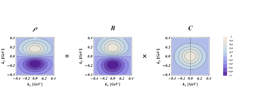
Figure 1: Simple illustration of the decomposition at fixed $x$ and $\bm{b}_{T}$. The phase-space distribution $\rho$ can be written as a product of a basic multipole $B$ (here a dipole in $\bm{k}_{T}$-space) with an oval-shaped coefficient function $C$.

$\rho_{X}$	$U$	$L$	$T_{x}$	$T_{y}$
$U$	$\langle 1\rangle$	$\langle S^{q}_{L}\ell^{q}_{L}\rangle$	$\langle S^{q}_{x}\ell^{q}_{x}\rangle$	$\langle S^{q}_{y}\ell^{q}_{y}\rangle$
$L$	$\langle S_{L}\ell^{q}_{L}\rangle$	$\langle S_{L}S^{q}_{L}\rangle$	$\langle S_{L}\ell^{q}_{L}S^{q}_{x}\ell^{q}_{x}\rangle$	$\langle S_{L}\ell^{q}_{L}S^{q}_{y}\ell^{q}_{y}\rangle$
$T_{x}$	$\langle S_{x}\ell^{q}_{x}\rangle$	$\langle S_{x}\ell^{q}_{x}S^{q}_{L}\ell^{q}_{L}\rangle$	$\langle S_{x}S^{q}_{x}\rangle$	$\langle S_{x}\ell^{q}_{x}S^{q}_{y}\ell^{q}_{y}\rangle$
$T_{y}$	$\langle S_{y}\ell^{q}_{y}\rangle$	$\langle S_{y}\ell^{q}_{y}S^{q}_{L}\ell^{q}_{L}\rangle$	$\langle S_{y}\ell^{q}_{y}S^{q}_{x}\ell^{q}_{x}\rangle$	$\langle S_{y}S^{q}_{y}\rangle$

Table 1: Correlations between target polarization ($S_{L},\bm{S}_{T}$), quark polarization ($S^{q}_{L},\bm{S}^{q}_{T}$) and quark OAM ($\ell^{q}_{L},\bm{\ell}^{q}_{T}$) encoded in the different phase-space distributions $\rho_{X}$.

It turns out that the contributions $\rho_{X}$ can be understood as encoding all the possible angular momentum correlations, see Table 1. Note that $\vec{\ell}^{q}$ refers to the canonical quark OAM, since it is defined in terms of the canonical quark momentum $\vec{k}$ [23]. The relation with the various angular correlations becomes particularly transparent once one sees the five-dimensional relativistic phase-space distributions as six-dimensional distributions integrated over the quark average longitudinal position $b_{L}=\vec{b}\cdot\hat{P}$ [18]

$$\rho_{X}(x,\bm{k}_{T},\bm{b}_{T};\hat{P},\eta)=\int\mathrm{d}b_{L}\,\rho_{X}(\vec{k},\vec{b};\hat{P},\eta).$$ (10)

Working at the level of phase-space distributions gives us much more insight about the physics encoded in the various GPDs and TMDs because integrations over $\bm{b}_{T}$ and $\bm{k}_{T}$ usually hide the precise form of the angular correlation being probed.

4 Representation of transverse phase space

Since we are essentially interested in the traverse phase space $(\bm{k}_{T},\bm{b}_{T})$, we reduce the number of variables by integrating the phase-space distributions $\rho_{X}$ over $x$ and discretizing the polar component of $\bm{b}_{T}$. The resulting transverse phase-space distributions are then represented as sets of distributions in $\bm{k}_{T}$-space

$$\rho_{X}(\bm{k}_{T}|\,\bm{b}_{T})=\int\mathrm{d}x\,\rho_{X}(x,\bm{k}_{T},\bm{b}_{T};\hat{P}=\vec{e}_{z},\eta=+1)\big{|}_{\bm{b}_{T}\text{ fixed}}$$ (11)

with the origin of axes lying on circles of radius $|\bm{b}_{T}|$ at polar angle $\phi_{b}$ in impact-parameter space, see Fig. 2. In this way, one can see how the transverse momentum is distributed at some point in the impact-parameter space.

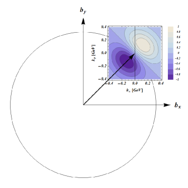
Figure 2: Representation of the transverse phase space. The circle represents the points in impact-parameter space at a fixed distance $|\bm{b}_{T}|$ from the center of the target. To each point on this circle is associated a distribution in transverse-momentum space. See text for more details.

This representation of transverse phase space has the advantage of making the multipole structure in both $\bm{k}_{T}$ and $\bm{b}_{T}$ spaces particularly clear. For example, the basic multipole $B^{(m_{k},m_{b})}_{X}$ will be represented by a $m_{k}$-pole in transverse-momentum space at any transverse position $\bm{b}_{T}$, with the orientation determined by $m_{b}$ and $\phi_{b}=\arg\hat{b}_{T}$. In the following, we chose to represent only eight points in impact-parameter space lying on a circle with radius $|\bm{b}_{T}|=0.4$ fm. Also, for a better legibility, the $\bm{k}_{T}$-distributions are normalized to the absolute maximal value over the whole circle in impact-parameter space

$$\max_{|\bm{b}_{T}|=0.4\text{ fm}}|\rho_{X}(\bm{k}_{T}|\bm{b}_{T})|=1.$$ (12)

5 Discussion

The results presented here are based on the light-front constituent quark model (LFCQM) [5] for up quarks. Light and dark regions correspond to positive and negative domains of the transverse phase-space distributions, respectively. Here we will focus on a couple of multipole structures only. The interested reader will find the complete discussion in Ref. [22].

5.1 $(0,0)$ multipole

The simplest multipole is naturally the one with $m_{k}=m_{b}=0$. It appears in $\rho^{e}_{X}$ with $X=UU,LL,TT$ associated to the respective spin structures $1$, $S_{L}S^{q}_{L}$ and $(\bm{S}_{T}\cdot\bm{S}^{q}_{T})$. These spin-spin correlations survive integration over $\bm{k}_{T}$ and $\bm{b}_{T}$; they are respectively related to $(H,\tilde{H},H_{T})$ in the GPD sector and to $(f_{1},g_{1},h_{1})$ in the TMD sector. Contrary to these GPDs and TMDs, $\rho^{e}_{X}$ is not circularly symmetric, see Fig. 3. The reason is that $\rho^{e}_{X}$ also contains information about the correlation between $\bm{k}_{T}$ and $\bm{b}_{T}$ (encoded in the coefficient functions $C^{e}_{X}$ through the $(\hat{b}_{T}\cdot\hat{k}_{T})^{2}$ dependence) which is lost under integration over $\bm{k}_{T}$ or $\bm{b}_{T}$ [3].

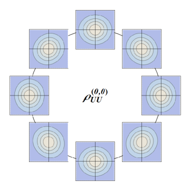
Figure 3: The $(0,0)$ multipole appearing in e.g. $\rho^{e}_{UU}$. See text for more details.

5.2 $(0,1)$ and $(1,0)$ multipoles

The first non-trivial multipoles are the ones with $m_{k}+m_{b}=1$.

The $(0,1)$ multipoles appear in $\rho^{e}_{X}$ with $X=UT,TU$ and in $\rho^{o}_{X}$ with $X=LT,TL$, see Fig. 4. In $\rho^{e}_{X}$, the $\bm{b}_{T}$-dipole is orthogonal to the transverse polarization $(\bm{S}^{q}_{T}\times\hat{b}_{T})_{L}$, $(\bm{S}_{T}\times\hat{b}_{T})_{L}$, and generates a shift in impact-parameter space which finds its physical origin in the intrinsic correlation between the transverse polarization and the quark OAM [24]. In $\rho^{o}_{X}$, the $\bm{b}_{T}$-dipole is parallel to the transverse polarization $S_{L}(\bm{S}^{q}_{T}\cdot\hat{b}_{T})$, $S^{q}_{L}(\bm{S}_{T}\cdot\hat{b}_{T})$, and is associated with an extrinsic double (longitudinal-transverse) spin-orbit correlation. These dipole structures do not survive integration over $\bm{b}_{T}$ and cannot therefore be accessed with TMDs. $\rho^{e}_{X}$ however survive integration over $\bm{k}_{T}$ and are then related to the GPDs $(2\tilde{H}_{T}+E_{T},E)$, respectively.

             

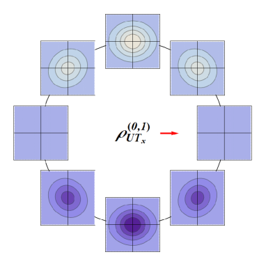
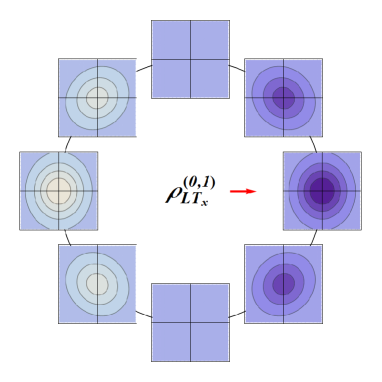
Figure 4: The $(0,1)$ multipoles appearing in e.g. $\rho^{e}_{UT}$ and $\rho^{o}_{LT}$. The arrow indicates the transverse polarization. See text for more details.

Similarly, the $(1,0)$ multipoles appear in $\rho^{e}_{X}$ with $X=LT,TL$ and in $\rho^{o}_{X}$ with $X=UT,TU$, see Fig. 5. In $\rho^{e}_{X}$, the $\bm{k}_{T}$-dipole is parallel to the transverse polarization $S_{L}(\bm{S}^{q}_{T}\cdot\hat{k}_{T})$, $S^{q}_{L}(\bm{S}_{T}\cdot\hat{k}_{T})$, and generates a shift in momentum space which is associated with an intrinsic double (longitudinal-transverse) spin-orbit correlation. In $\rho^{o}_{X}$, the $\bm{k}_{T}$-dipole is orthogonal to the transverse polarization $(\bm{S}^{q}_{T}\times\hat{k}_{T})_{L}$, $(\bm{S}_{T}\times\hat{k}_{T})_{L}$, and indicates the presence of a net transverse flow originating from an extrinsic correlation between the transverse polarization and the quark OAM, reminiscent of a quantum Hall effect. These dipole structures do not survive integration over $\bm{k}_{T}$ and cannot therefore be accessed with GPDs. $\rho^{e}_{X}$ and $\rho^{o}_{X}$ however survive integration over $\bm{b}_{T}$ and are then related to the TMDs $(h^{\perp}_{1L},g_{1T})$ and $(h^{\perp},f_{1T}^{\perp})$, respectively.

             

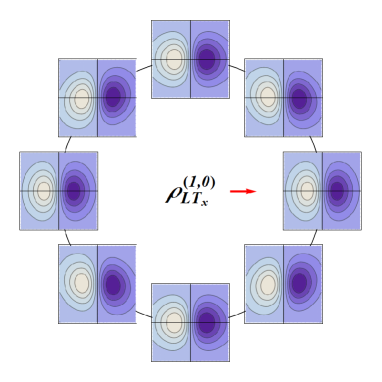
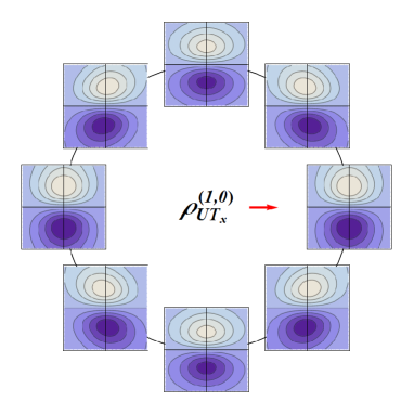
Figure 5: The $(1,0)$ multipoles appearing in e.g. $\rho^{e}_{LT}$ and $\rho^{o}_{UT}$. The arrow indicates the transverse polarization. See text for more details.

5.3 $(1,1)$ multipoles

The last multipoles we will discuss here are the ones with $m_{k}=m_{b}=1$. Since $m_{k}=m_{b}$, these multipoles are invariant under rotation about the longitudinal direction. They appear in $\rho^{e}_{X}$ with $X=UL,LU$ and $\rho^{o}_{X}$ with $X=UU,LL,TT,TT^{\prime}$, see Fig. 6. In $\rho^{e}_{X}$ and $\rho^{o}_{TT^{\prime}}$, the $\bm{k}_{T}$-dipole is oriented along the polar direction $S^{q}_{L}(\hat{b}_{T}\times\hat{k}_{T})_{L}$, $S_{L}(\hat{b}_{T}\times\hat{k}_{T})_{L}$ and $(\bm{S}_{T}\times\bm{S}^{q}_{T})_{L}(\hat{b}_{T}\times\hat{k}_{T})_{L}$. Clearly, $\rho^{e}_{X}$ is related to the orbital motion of quarks correlated with the longitudinal polarization [3, 7, 8, 9, 10, 11]. $\rho^{o}_{TT^{\prime}}$ is less transparent as it originates from an extrinsic double (transverse-transverse) spin-orbit correlation. In $\rho^{o}_{X}$ with $X=UU,LL,TT$, the $\bm{k}_{T}$-dipole is oriented along the radial direction $(\hat{b}_{T}\cdot\hat{k}_{T})$, $S_{L}S^{q}_{L}(\hat{b}_{T}\cdot\hat{k}_{T})$ and $(\bm{S}_{T}\cdot\bm{S}^{q}_{T})(\hat{b}_{T}\cdot\hat{k}_{T})$, and indicates a net expansion or contraction of the target in the transverse plane as a consequence of the initial and/or final-state interactions, the most simple manifestation of the lensing effect in QCD. Unfortunately, none of these structures survive integration over $\bm{k}_{T}$ or $\bm{b}_{T}$ and cannot therefore be accessed with GPDs or TMDs.

             

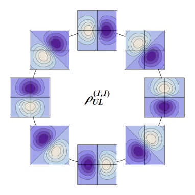
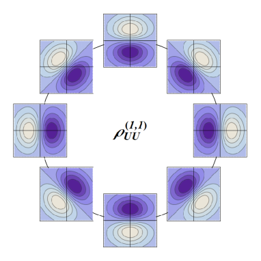
Figure 6: The $(1,1)$ multipoles appearing in e.g. $\rho^{e}_{UL}$ and $\rho^{o}_{UU}$. See text for more details.

6 Conclusions

We presented and discussed a selection of leading-twist quark Wigner distributions in the nucleon, introducing a multipole analysis in the transverse phase space. In this approach, the multipole structures are constrained by parity and time-reversal symmetries and are multiplied by coefficient functions which depend on $\mathsf{P}$ and $\mathsf{T}$-invariant variables only. This representation has several advantages: it provides a clear interpretation of all the amplitudes in terms of the possible correlations between target and quark angular momenta in the transverse phase space, and it provides a convenient basis to make a direct connection with GPDs in impact-parameter space and TMDs in transverse-momentum space. A new graphical representation has also been proposed to display these transverse phase-space distributions.

We presented results for a few lowest multipole structures in both impact-parameter and transverse momentum spaces, half of them being naive $\mathsf{T}$-even and representing the intrinsic structure of the target, the other half being naive $\mathsf{T}$-odd and representing the response of the target to extrinsic initial and/or final-state interactions. These structures have been confirmed and calculated within a light-front consituent quark model

- [1] X. d. Ji, Viewing the proton through ’color’ filters, Phys. Rev. Lett. 91 (2003) 062001 [hep-ph/0304037].
- [2] A. V. Belitsky, X. d. Ji and F. Yuan, Quark imaging in the proton via quantum phase space distributions, Phys. Rev. D 69 (2004) 074014 [hep-ph/0307383].
- [3] C. Lorcé and B. Pasquini, Quark Wigner Distributions and Orbital Angular Momentum, Phys. Rev. D 84 (2011) 014015 [arXiv:1106.0139 [hep-ph]].
- [4] S. Meissner, A. Metz and M. Schlegel, Generalized parton correlation functions for a spin-1/2 hadron, JHEP 0908 (2009) 056 [arXiv:0906.5323 [hep-ph]].
- [5] C. Lorcé, B. Pasquini and M. Vanderhaeghen, Unified framework for generalized and transverse-momentum dependent parton distributions within a 3Q light-cone picture of the nucleon, JHEP 1105 (2011) 041 [arXiv:1102.4704 [hep-ph]].
- [6] C. Lorcé and B. Pasquini, Structure analysis of the generalized correlator of quark and gluon for a spin-1/2 target, JHEP 1309 (2013) 138 [arXiv:1307.4497].
- [7] Y. Hatta, Notes on the orbital angular momentum of quarks in the nucleon, Phys. Lett. B 708, (2012) 186 [arXiv:1111.3547 [hep-ph]].
- [8] C. Lorcé, B. Pasquini, X. Xiong and F. Yuan, The quark orbital angular momentum from Wigner distributions and light-cone wave functions, Phys. Rev. D 85 (2012) 114006 [arXiv:1111.4827 [hep-ph]].
- [9] K. Kanazawa, C. Lorcé, A. Metz, B. Pasquini and M. Schlegel, Twist-2 Generalized TMDs and the Spin/Orbital Structure of the Nucleon, Phys. Rev. D 90 (2014) 014028 arXiv:1403.5226 [hep-ph].
- [10] C. Lorcé, Spin–orbit correlations in the nucleon, Phys. Lett. B 735 (2014) 344 [arXiv:1401.7784 [hep-ph]].
- [11] K. F. Liu and C. Lorcé, The Parton Orbital Angular Momentum: Status and Prospects, Eur. Phys. J. A 52, no. 6 (2016) 160 [arXiv:1508.00911 [hep-ph]].
- [12] A. D. Martin, M. G. Ryskin and T. Teubner, Q**2 dependence of diffractive vector meson electroproduction, Phys. Rev. D 62 (2000) 014022 [hep-ph/9912551].
- [13] V. A. Khoze, A. D. Martin and M. G. Ryskin, Can the Higgs be seen in rapidity gap events at the Tevatron or the LHC?, Eur. Phys. J. C 14 (2000) 525 [hep-ph/0002072].
- [14] A. D. Martin and M. G. Ryskin, Unintegrated generalized parton distributions, Phys. Rev. D 64 (2001) 094017 [hep-ph/0107149].
- [15] M. G. Albrow et al. [FP420 R and D Collaboration], The FP420 & Project: Higgs and New Physics with forward protons at the LHC, JINST 4 (2009) T10001 [arXiv:0806.0302 [hep-ex]].
- [16] A. D. Martin, M. G. Ryskin and V. A. Khoze, Forward Physics at the LHC, Acta Phys. Polon. B 40 (2009) 1841 [arXiv:0903.2980 [hep-ph]].
- [17] Y. Hatta, B. W. Xiao and F. Yuan, Probing the Small- x Gluon Tomography in Correlated Hard Diffractive Dijet Production in Deep Inelastic Scattering, Phys. Rev. Lett. 116, no. 20 (2016) 202301 [arXiv:1601.01585 [hep-ph]].
- [18] C. Lorcé and B. Pasquini, Multipole decomposition of the nucleon transverse phase space, Phys. Rev. D 93, no. 3 (2016) 034040 [arXiv:1512.06744 [hep-ph]].
- [19] M. G. Echevarria, A. Idilbi, K. Kanazawa, C. Lorcé, A. Metz, B. Pasquini and M. Schlegel, Proper definition and evolution of generalized transverse momentum dependent distributions, Phys. Lett. B 759 (2016) 336 [arXiv:1602.06953 [hep-ph]].
- [20] C. Lorcé and B. Pasquini, On the Origin of Model Relations among Transverse-Momentum Dependent Parton Distributions, Phys. Rev. D 84 (2011) 034039 [arXiv:1104.5651 [hep-ph]].
- [21] M. Diehl and P. Hägler, Spin densities in the transverse plane and generalized transversity distributions, Eur. Phys. J. C 44 (2005) 87 [hep-ph/0504175].
- [22] C. Lorcé, The light-front gauge-invariant energy-momentum tensor, JHEP 1508 (2015) 045 [arXiv:1502.06656 [hep-ph]].
- [23] C. Lorcé, Wilson lines and orbital angular momentum, Phys. Lett. B 719 (2013) 185 [arXiv:1210.2581 [hep-ph]].
- [24] M. Burkardt, Transverse deformation of parton distributions and transversity decomposition of angular momentum, Phys. Rev. D 72 (2005) 094020 [hep-ph/0505189].