Abstract

Novel bound states are obtained for manifolds with singular potentials. These singular potentials require proper boundary conditions across boundaries. The number of bound states match nicely with what we would expect for blackholes. Also they serve to model membrane mechanism for the blackhole horizons in simpler contexts. The singular potentials can also mimic expanding boundaries elegantly, there by obtaining appropriately tuned radiation rates.

Modelling quantum black hole

T. R. Govindarajan

Chennai Mathematical Institute, H1, SIPCOT IT Park, Kelambakkam, Siruseri 603103, India

J.M. Munõz-Castañeda

Physics Department, ETSIAE Universidad Politécnica de Madrid,Spain

1 Introduction

W. Pauli [1]remarked the boundaries were the creation of the devil. Bekenstein’s area law [2, 3] for the entropy of blackhole prescribes that the microscopic states live close to the horizon and the number of such states grow rapidly with area. One can proceed at least in the case of large blackholes without the detailed requirements of quantum geometry to study quantum blackholes. Such attempts have been made earlier by ’t Hooft through a brick wall [4], and Beckenstein and Mukhanov[5]. The entropy is understood in some context by entanglement of those inside the horizon which are inaccessible to asymptotic observer with the outside[6, 7].

In this communication we elaborate an earlier proposal[8] by one of us that the existence of bound states in the blackhole geometries resulting from the study of self adjoint extensions of the Laplacian near the horizon. Near horizon geometry of blackholes present a singular potential to the particles and can be studied through quantum mechanics with special boundary conditions. Not only they lead to localised states on the boundary their number also scales like area. This in statistical mechanics or in quantum field theory (QFT) context translates as entropy [9]. Similar is the case of von Neumann entropy when we trace over unobserved bound states for a distant observer. The quantum physics on manifolds with boundaries introduces novel features. They appear in varied situations like Casimir effect [10, 11, 12, 13], quantum hall, topological insulators[14, 15] or quantum gravity contexts like blackhole, or de Sitter spacetime with cosmological horizon [16, 17]. Many of the novel features stem from studying correct boundary conditions which are physically relevant as well mathematically correct to make the Hamiltonian a self adjoint operator in properly extended domains in the Hilbert space of $L^{2}$ functions.

The garden variety boundary conditions are Dirichlet and Neumann for which either the function or the normal derivative vanishes. However as shown for the Laplacian a more general class of boundary condition is possible, a particular example being Robin boundary condition. Here the function and the normal are related on the boundary $(\psi~{}+~{}\kappa\partial\psi)|_{\partial{\cal{M}}}~{}=~{}0$. Dirichlet and Neumann are extreme limits of the Robin boundary condition. But more importantly it introduces a fundamental length $\kappa$ into the theory[18, 19]. Such a parameter will emerge from the coarse grained structure of the underlying space-time or crystalline lattice. Typically it can be related to Planck length in a semiclassical gravity context.

But the boundaries are obtained in reality through singular potentials or point interactions in space-time and such potentials are also subjected to self adjointness conditions on unbounded operators[20, 21, 22]. The well known potential of this kind in one dimension is the $\delta(x)$ which introduces discontinuity in the derivative of the wavefunctions. More general potentials of the same type is the $\delta^{\prime}(x)$ potential which has the new feature of introducing discontinuities in the wavefunction itself. Inspite of such discontinuities the Hamiltonian remains self adjoint and the quantum theory describes well defined unitary evolution. This approach allows study of quntum fields over bounded regions in terms of interesting and meaningful questions that can be answered. One can sacrifice the self adjointness with special boundary conditions like purely ingoing waves leading to quasi normal modes (QNM) which are also linked to ringing modes of stellar objects including blackholes. [23].

We will consider quantum theory with point interactions of the type which is a combination of $\delta$ and $\delta^{\prime}$ potentials. Such a combination in addition to being more general, is also necessitated for several reasons. They arise naturally when we consider self adjoint extensions of Dirac operator with singular $\delta$ potential [24]. But for us it brings new features like what we anticipate from membrane paradigm[16, 17]for black holes through a new parameter. Our constructions can easily be extended to curved backgrounds too.

Introduction of singular distributions as potentials also help in introducing time dependent boundaries and associated radiation. We will study in this communication in Sec 2 a model Schrodinger equation in $R^{2}$ wih singular point interaction potentials $a\delta(r-R)~{}+~{}2b\delta^{\prime}(r-R)$. We consider in Sec 2a the scattering states and in Sec 2b the bound states. In Sec 2c we explain the extension to 3 dimensions. We also remark about BTZ blackhole in this context. In Sec 3 we consider moving boundaries through singular potentials and explain how this program can be carried out[25].

2 The model

The general study of point interactions of the free Hamiltonian in one dimension $H~{}=~{}\frac{\hbar^{2}}{2m}\frac{d^{2}}{dx^{2}}$ is due to Kurasov [26, 27] and uses von Neumann’s theory of symmetric unbounded operators with identical deficiency indices[20]. The general analysis of self adjointness of Laplacian in higher dimensional manifolds with boundaries is more complex due to infinite deficiency indices. But it is possible to relate them directly to boundary conditions of functions and normal derivatives on the boundaries[21, 22]. In cases like ours, the presence of isometries simplifies the problem considerably and provide exact solutions [18].

Consider a Schrodinger Hamiltonian equation in $R^{2}$ for stationary states with a singular potential along a circle of radius $R$:

$$\left[-\frac{\hbar^{2}}{2m}\Delta+a\delta(r-R)+b\delta^{\prime}(r-R)\right]\Psi(r,\theta)=E\Psi(r,\theta)$$ (1)

In order to work with dimensionless quantities, let us introduce new variables and parameters.

$${\bf r}=\frac{\hbar}{mc}\,{\bf x},\ R~{}=~{}\frac{\hbar}{mc}\,X,\ w_{0}=\frac{2a}{\hbar c},\ w_{1}=\frac{mb}{\hbar^{2}},\ \lambda=\frac{2E}{mc^{2}},\$$ (2)

such that (1) becomes with $\varphi({\bf x})=\Psi(r,\theta)$,

$$-\Delta_{\bf x}\,\varphi({\bf x})+w_{0}\delta(x-X)\varphi({\bf x})+2w_{1}\delta^{\prime}(x-X)\varphi({\bf x})=\lambda\,\varphi({\bf x}).$$ (3)

This new parametrization corresponds to lengths being measured in the units of Compton wavelength of the particle. The origin of $a$ is related to the underlying background geometry and is independent of ‘m’. On the other hand ‘b’ is related to the mass ‘m’.

The crucial question is to find the domain of wave functions $\varphi({\bf x})$ that makes $H_{0}$ self adjoint. As these functions and their derivatives have a discontinuity at $x=X$, we have to define the products of the form $\delta(x-X)\varphi({\bf x})$ and $\delta^{\prime}(x-X)\varphi({\bf x})$ in (1). The form for these products are given as:

$$\delta(x-X)\varphi({\bf x}) = \frac{\varphi(X^{+},\theta)+\varphi({X}^{-},\theta)}{2}\,\delta({x-X})\,,$$

$$\delta^{\prime}({x-X})\varphi({\bf x}) = \frac{\varphi({X}^{+},\theta)+\varphi({X}^{-},\theta)}{2}\,\delta^{\prime}({x-X})$$ (4)

$$- \frac{\varphi^{\prime}({X}^{+},\theta)+\varphi^{\prime}({X}^{-},\theta)}{2}\,\delta({x-X})$$

where $f({X}^{+},\theta)$ and $f({X}^{-},\theta)$ are the right and left limits of the function $f({\bf x})$ as ${x}\to{X}$, respectively. The problem is separable and can be reduced to a 1D radial problem with a central potential. In order to obtain a self-adjoint extension of the Hamiltonian we have to find a domain on which this extension acts, namely given by a space of square integrable functions satisfying matching conditions at the point $X$. The radial functions in the domain of the Hamiltonian $H$ are functions in the Sobolev space $W^{2}_{2}({\mathbb{R}}/\{S^{2}(X)\})$ such that at $x=X$ satisfy the following matching conditions given by an $SL(2,R)$ matrix[28]:

$$\left(\begin{array}[]{c}\varphi(X^{+})\\[4.30554pt] \varphi^{\prime}(X^{+})\end{array}\right)=\left(\begin{array}[]{cc}\displaystyle\frac{1+w_{1}}{1-w_{1}}&0\\[4.30554pt] \displaystyle\frac{w_{0}}{1-w_{1}^{2}}&\displaystyle\frac{1-w_{1}}{1+w_{1}}\end{array}\right)\left(\begin{array}[]{c}\varphi(X^{-})\\[4.30554pt] \varphi^{\prime}(X^{-})\end{array}\right)\,.$$ (5)

Note that in the case of $w_{1}$ being zero it goes to known discontinuities in normal derivatives [24].

2.1 Scattering states

For scattering theory we solve Schrodinger equation with plane waves and positive energy $k^{2}$. For each angular momentum $n$ we obtain the following Schrödinger 1D problem for $\varphi(r,\theta)~{}=~{}{\cal{R}}~{}e^{in\theta}$ :

$$\frac{d^{2}{\cal{R}}}{dr^{2}}+\frac{1}{r}\frac{d{\cal{R}}}{dr} + \left(w_{0}\delta(r-R)+2w_{1}\delta^{\prime}(r-R)\right){\cal{R}}$$ (6)

$$- \left(\lambda+\frac{n^{2}}{r^{2}}\right){\cal{R}}=0$$

with $\lambda~{}=-~{}k^{2}$ and suitable boundary conditions. The general scattering solution is given by

$${\cal{R}}(r)=\begin{cases}J_{n}(kr)&r<R\\ A(k,n)J_{n}(kr)+B(k,n)Y_{n}(kr)&r>R\end{cases},$$ (7)

where $J_{n}$ and $Y_{n}$ are the Bessel functions, $A(k,n)$ and $B(k,n)$ constants to be determined through matching boundary conditions.

$$B(k,n) = J_{n}(x)\left(4kw_{1}~{}R~{}J_{n-1}(x)-J_{n}(x)\left(4w_{1}n~{}+~{}w_{0}R\right)\right)$$

$$A(k,n) = J_{n}(x)\left(k(w_{1}+1)^{2}RY_{n-1}(x)-Y_{n}(x)\left(4w_{1}L+w_{0}R\right)\right)$$

$$- k(w_{1}-1)^{2}R~{}J_{n-1}(x)Y_{n}(x)$$

where we have defined $x~{}=~{}kR$. This complicated looking expression can be checked to coincide with expected results for hard sphere ($w_{1}~{}=~{}-1$). Note that when $w_{1}=1$ the exterior side of the Disc $D_{2}$ is seen by the quantum particle as Robin boundary condition while the inside face is Dirichlet. On the other hand for $w_{1}=-1$ this is the other way round. The phase shifts are given by $\tan(\delta_{n})=-B(k,n)/A(k,n)$[29] where $A,B$ are given above.

2.2 Bound states

The Schrodinger equation is Eq. (6) with $\lambda~{}\geq~{}0$. The solutions in the regions $r~{}<~{}R~{}and~{}r~{}>~{}R$ are the modified Bessel functions of the first and second kind: ${\cal{R}}(r)~{}=~{}c~{}I_{n}(\sqrt{\lambda}r)$ and $d~{}K_{n}(\sqrt{\lambda}r)$. We match the boundary conditions at $r~{}=~{}R$ using Eq.5. We rewrite: $\alpha~{}=\frac{1+\omega_{1}}{1-\omega_{1}},~{}~{}\beta~{}=~{}\frac{2\omega_{0}}{1-w_{1}^{2}}$. We get (with $x~{}=~{}\sqrt{\lambda}R$),

$$x\left(\alpha\frac{K_{n}^{\prime}(x)}{K_{n}(x)}~{}-~{}\alpha^{-1}\frac{I_{n}^{\prime}(x)}{I_{n}(x)}\right)~{}=~{}\bar{\beta}$$ (8)

where $\bar{\beta}~{}=~{}\beta~{}R$. We can simplify the above equation using Bessel function identities to get:

$$-x\left(\frac{\alpha~{}K_{n-1}}{K_{n}}~{}+~{}\frac{\alpha^{-1}I_{n-1}}{I_{n}}\right)~{}-~{}n~{}(\alpha~{}-~{}\alpha^{-1})=~{}\bar{\beta}$$ (9)

Now we can look for a maximum value of $n~{}=~{}n_{m}$. It is easy to work out: This gives:

$$-~{}n_{m}~{}(\alpha~{}+~{}\alpha^{-1})~{}=~{}\bar{\beta}$$ (10)

Hence the maximum number of bound states are still proportional to the radius of the circle, but with a renormalised constant $\frac{w_{0}}{2(1~{}+~{}w_{1}^{2})}$. For the special case of $w_{1}~{}=~{}0$ we get maximum number $n_{m}$ of bound states is the nearest integer lower than $\bar{w}_{0}$, which is same as our earlier result[8, 18]. For the case when $w_{1}$ is small when we can drop $w_{1}^{2}$ term we get the number of bound states is unaltered. This is to be expected since the singular potential can be written as shifted singular potential: $V(r)~{}\approx~{}w_{0}~{}\delta(r-R~{}+~{}\frac{2w_{1}}{w_{0}})$.

Energy eigenvalues are obtained numerically for different values $R,w_{0}$ and $w_{1}$ by solving Eq.(9). Similarly we obtain expectation values $<r_{n}>$ by using appropriate ${\cal{R}}(r)$ in the two regions. The graphs demonstrate the number of bound states as well as energy eigenvalues (Fig.2). They also explicitely show that they are localised close to the boundary and deviate externally or internally when we increase the coefficent of $\delta^{\prime}$ potential (Fig.2,3). Interestingly the states are localised outside (inside) the boundary for positive (negative) $w_{1}$ respectively. $w_{1}$ can be tuned to reduce the probability of finding the particle inside model blackhole to be small. Also note that higher angular momenta states move closer to (away from ) the boundary for negative (positive) $w_{1}$. We will remark about this in the conclusions.

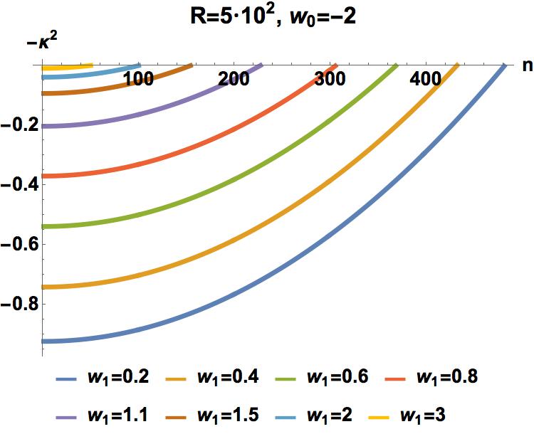
Figure 1: Bound states $E(w_{1})$

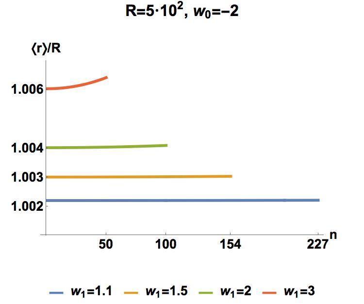
Figure 2: $<r_{n}>/R$ for large $w_{1}$

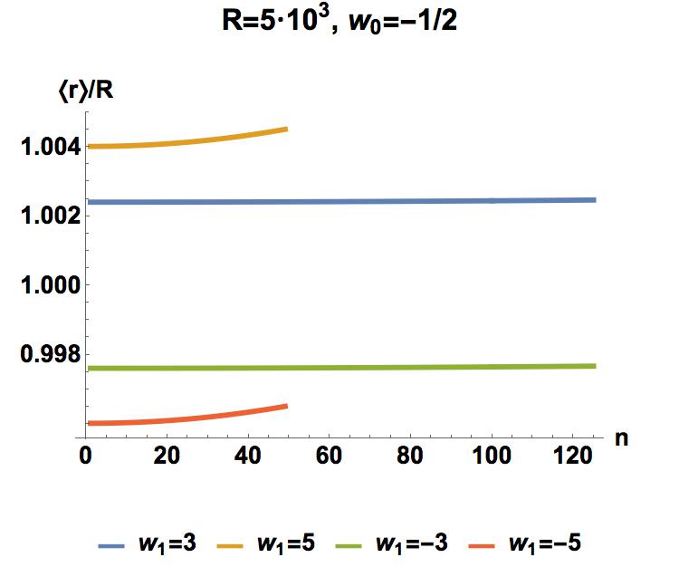
Figure 3: Expectation $<r_{n}>/R$ for large R

2.3 Three dimensions and BTZ blackhole:

We present in this section the results for bound states in $d~{}=~{}3$. For that we consider Schrodinger equation on $R^{3}$ with a singular potential along a sphere: $V(r)~{}=~{}a\delta(r-R)~{}+~{}2b~{}\delta^{\prime}(r-R)$. The required Schrodinger equation in spherical polar coordinates has solutions $\varphi(r,\theta,\phi)~{}=~{}{\cal{R}}(r)Y_{lm}(\theta,\phi)$ where $Y_{lm}$ are spherical harmonics solving angular part of the equations. The radial part of the equation is:

$$\frac{d^{2}{\cal{R}}}{dr^{2}}~{}+~{}\frac{2}{r}\frac{d{\cal{R}}}{dr}~{}-~{}\frac{l(l+1){\cal{R}}}{r^{2}}~{}=~{}\lambda{\cal{R}}$$ (11)

The solutions in the regions $r~{}<~{}R~{}and~{}r~{}>~{}R$ are modified spherical Bessel functions: ${\cal{R}}(r)~{}=~{}c~{}\frac{I_{l+\frac{1}{2}}(\sqrt{\lambda}r)}{\sqrt{r}}$ and  $d~{}\frac{K_{l+\frac{1}{2}}(\sqrt{\lambda}r)}{\sqrt{r}}$. Again matching the boundary conditions at $r~{}=~{}R$ and using Eq.5, the Eq.(9) gets modified to:

$$-x\left(\frac{\alpha K_{l-\frac{1}{2}}}{K_{l+\frac{1}{2}}}+\frac{\alpha^{-1}I_{l-\frac{1}{2}}}{I_{l+\frac{1}{2}}}\right)-(l+1)(\alpha-\alpha^{-1})=\bar{\beta}$$ (12)

The maximum angular momentum allowed $l_{max}~{}=~{}\frac{\bar{\beta}+\alpha}{\alpha~{}+~{}\alpha^{-1}}$. Each angular momentum $l$ has degeneracy of $2l~{}+~{}1$ states. Hence the number of states upto $l_{max}~{}\propto 2l_{max}^{2}$ we get the number of bound states $\propto R^{2}$.

We will briefly mention the toy model of blackhole in 3d, BTZ blackhole [30, 31] For simplicity we consider BTZ blackhole metric with angular momentum $J~{}=~{}0$. The metric is given by:

$$ds^{2}=-\left(\frac{r^{2}}{l^{2}}-M\right)dt^{2}+\left(\frac{r^{2}}{l^{2}}-M\right)^{-1}dr^{2}+r^{2}d\phi^{2}$$ (13)

Here cosmological constant $\frac{1}{l^{2}}$ and $M$ is the mass of the blackhole and horizon is at $r~{}=~{}r_{+}~{}=~{}\sqrt{M}l$. The solution of the scalar field in the presence of this metric along with singular potentials $\delta(r-r_{+})$ and $\delta^{\prime}(r-r_{+})$ can be written as: $e^{-i\omega t~{}+im\phi}{\cal{R}}(r)$. Defining, $z~{}=~{}\frac{r^{2}~{}-~{}r_{+}^{2}}{r^{2}},~{}~{}~{}~{}{\cal{F}}(z)~{}=~{}z^{i\alpha}(1-z)^{-\beta}{\cal{R}}(z)$ one gets the hypergeometric differential equation for ${\cal{F}}(z)$:

$$z(1-z)\frac{d^{2}{\cal{F}}}{dz^{2}}~{}+~{}(c-~{}(1+a+b))\frac{d{\cal{F}}}{dz}~{}+~{}ab{\cal{F}}~{}=~{}0$$ (14)

where $a,b,c,\alpha,\beta$ are constants defined terms of $r_{+},l,m,\omega$. This hypergeometric equation has singularities at $z=0,1$. To obtain the bound states one should match the boundary conditions at $z=0$ for the hypergeometric functions ${\cal{F}}(a,b,c,z)$.

3 Expanding boundaries

In this brief section we explore the singular potentials for introduction of time dependence in boundaries. The simple case of in one dimension with $x~{}>~{}0$: If the boundary is moving with uniform velocity like $x~{}=~{}vt$ it can be studied as a quntum mechanical problem with delta function potential $\delta(x-vt)$. The solution is easy to get as $\psi(x,t)~{}\propto~{}e^{-|\kappa(x-vt)|}e^{-i(\kappa^{2}-v^{2}/2)t-vx}$.

We can easily extend this analysis to a boundary with an acceleration ‘g’ with a singular potential $\delta(x-\frac{gt^{2}}{2})$. This is unitarily equivalent to the static singular potential and an additional gravitional potential $mgx$. This can be seen by using the unitary transformations: $\phi(x,t)~{}=~{}U~{}V~{}\psi(x,t)$ where $V(x,t)~{}=~{}e^{-i\frac{g^{2}t^{2}p_{x}}{2}},~{}~{}U(x,t)~{}=~{}e^{igxt~{}+~{}i\frac{g^{2}t^{3}}{6}}$ The solutions for linear gravitational potential are given by Airy functions.

Similarly we can consider $R^{2}~{}-~{}D$. If the disc is expanding it is better to convert the question to a delta function potential which is expanding.

Berry and Klein [32] showed the time dependent

$$H(r,p,l(t))=\frac{p^{2}}{2m}+\frac{1}{l^{2}}V(r/l).$$ (15)

can be simplified if the time dependence is of the form $l(t)=\sqrt{at^{2}+2bt+c}$. It becomes in a comoving frame:

$$H(\rho,\pi,k)=\frac{\pi^{2}}{2m}+V(\rho)+\frac{1}{2}k\rho^{2},$$ (16)

where $\rho=r/l$ and $k=m(ac-b^{2})$ which is conserved in $\rho,\tau\equiv\int^{t}\frac{dt}{l^{2}(t)}$. The expanding disc in $\mathbb{R}^{2}$ and ball in $\mathbb{R}^{3}$ will come under this class of Hamiltonians. Consider the Hamiltonian [18] in $R^{2}$

$$H~{}=~{}-\Delta~{}+~{}g~{}\delta(r~{}-~{}e^{f}R(0))~{}$$ (17)

By rescaling r we get the potential as $e^{f}\delta(r~{}-~{}R(0))$. The time dependence is shifted to the strength of potential. This is analogous to changing the Hamiltonian to a time dependent one by keeping the domain of the wavefunctions in the Hilbert space same for all times.

Applying Berry, Klein transformation [32] we can convert the problem in a comoving frame to a time independent potential with a delta function along a ring. This will also correspond to generalised pantographic change of Fabio Anza etal [33] This has important consequesnces for the rate of emission or in expanding statistical ensembles with new boundary conditions.

4 Conclusions

In this report we have approached the question of quantum blackhole through straightforward analysis of quantum theory on manifolds with boundaries or equivalently singular potentials. While our study is in Euclidean space it can be applied to curved background also since point interactions are local. This can parallel the recent approach to understand blackholes through conventional notions of particles and forces treating blackholes just like atoms, molecules (see ’t Hooft[34]). These require analysis through self adjoint extensions of operator domains. Our analysis surprisingly brings out the importance of both $\delta$ and $\delta^{\prime}$ potentials. There are a number bound states localised close to the boundary and is proportional to the area. As pointed out in the Introduction [9] they relate to entropy in QFT. Hence the existence of correct behaviour of localised bound states on the boundary is a strong requirement for correct entropy. We also point out the role of $\delta^{\prime}$ potential in extending the support of the bound states to enhanced length scales to allow for the possibility of quantum effects beyond Planck length[35].

Following tHooft [4] one can consider scalar fields to vanish at a small distance away from the horizon. That is $\phi(R+h)~{}=~{}0$. This is for small $h$ equivalent to Robin boundary condition since by expanding around R we get $\phi(R)~{}+~{}h\phi^{\prime}(R)~{}\approx 0$. This boundary condition can also be obtained from $\delta$ function potential. Our potential is a generalisation of the potential which adds another parameter which allows the quantum effects to persist beyond the length parameter $h$. In Kruskal coordinates one avoids the singularity of the metric at the horizon, but contain two copies of the space time. This is mimicked in our case of singular potentials connecting the two regions with suitable boundary conditions to maintain unitarity. Our generalised brickwall mechanism can be studied to obtain all the thermodynamic properties. Detailed analysis using these boundary conditions for the thermodynamic behaviour will be presented elsewhere with Rindler, BTZ and Schwardschild background(under preparation).

These states are interestingly connected through spectrum generating algebra which is a sub algebra of the Schrodinger group. By tuning the strength of the $\delta^{\prime}$ potential one can control the tunnelling through the boundary. Lastly if we scale the radius to $\infty$ keeping number of bound states fixed ($\frac{w_{0}}{w_{1}^{2}}\rightarrow 0$) the states become zero energy bound states and localised at the boundary and play signifcant role for asymptotic symmetries. The connections to QNM which arise from purely ingoing modes is also intriguing. In addition the singular potentials can be time dependent to enable the analysis of expanding boundaries and associated radiation output. This study leads us to new avenues of exploration to situations where boundaries and boundary conditions are involved[25].

Acknowledgements: TRG and JMMC thank Manuel Asorey,University of Zaragoza. TRG acknowledges discussions with Rakesh Tibrewala. JMMC acknowledge the funding by Spanish Government (project MTM2014-57129-C2-1-P) and discussions with L. M. Nieto, M. Gadella, and K.Kirsten.

References

- [1] Growth, Dissolution and Pattern Formation in Geosystems, B. Jamtveit and P. Meakin (Kluwer Academic Publishers, Dordrecht, 2010).
- [2] J.D. Bekenstein, Phys. Rev. D 7, 2333 (1973).
- [3] S.W. Hawking, Comm. Math. Phys. 43, 199 (1975).
- [4] G. ’t Hooft, Nucl. Phys. B 256, 727 (1985).
- [5] J.D. Bekenstein and V.F. Mukhanov, Phys.Lett.B 360,7(1995).
- [6] L.Bombelli, R.K. Koul, J. Lee and R.D. Sorkin, Phys. Rev. D 34, 373 (1986).
- [7] M. Srednicki, Phys. Rev. Lett. 71, 666 (1993);
- [8] T.R. Govindarajan, V. Suneeta and S. Vaidya, Nucl. Phys. B 583, 291 (2000),
- [9] J. Wheeler, It from bit, Sakharov Memorial Lecture on Physics, vol. 2, L. Keldysh and V. Feinberg, Nova (1992)
- [10] J. Mateos Guilarte and J. M. Muñoz-Castañeda, Int. J. Theor. Phys. 50, 2227 (2011).
- [11] J. M. Muñoz-Castañeda, J. Mateos Guilarte, and A. Moreno Mosquera, Phys. Rev. D 87, 105020 (2013),
- [12] J. M. Muñoz-Castañeda and J. Mateos Guilarte, Phys.Rev. D91 025028 (2015),
- [13] D. Karabali and V. P. Nair, Phys. Rev. D 87, 105021 (2013).
- [14] M. Z. Hasan and C. L. Kane, Rev. Mod. Phys. 82, 3045 (2010),
- [15] M. Asorey, A. P. Balachandran, and J. M. Prez-Pardo, J. High Energy Phys. 12 (2013) 073.
- [16] Black Holes: The Membrane Paradigm, edited by K. S. Thorne, R. H. Price, and D. A. Macdonald (Yale University Press, London, 1986,
- [17] T. Damour, Phys. Rev. D 18, 3598 (1978)
- [18] T. R. Govindarajan and R. Tibrewala, Phys. Rev. D 83, 124045 (2011),
- [19] T. R. Govindarajan and V. P. Nair, Phys. Rev. D 89, 025020 (2014).
- [20] M. Reed and B. Simon, Methods of Modern Mathematical Physics Vol. I-IV (Academic Press) (1980).
- [21] M. Asorey, A. Ibort and G. Marmo, Int.J.Geom.Meth.Mod.Phys. 12 1561007 (2015),
- [22] M. Asorey and J.M. Muñoz-Castañeda, Nucl.Phys. B 874, 852 (2013),
- [23] Kostas D. Kokkotas, Bernd G. Schmidt, Living Rev.Rel.2:2 (1999)
- [24] T. R. Govindarajan, and R. Tibrewala, Phys. Rev D92, 045040 (2015).
- [25] T R Govindarajan and J. M. Muñoz-Castañeda, under preparation.
- [26] P. Kurasov, Journal of Mathematical Analysis and Applications 201, 297 (1996).
- [27] Solvable models in quantum mechanics, Albeverio, S. and Gesztesy, F. and Høegh-Krohn, R. and Holden, H, AMS Chelsea Publishing, Providence, RI (2005)
- [28] M. Gadella and J. Negro and L.M. Nieto, Physics Letters A 373, 1310 (2009)
- [29] I. Richard Lapidus, American Journal of Physics, 50, 45 (1982).
- [30] M. Banados, C. Teitelboim and J. Zanelli, Phys. Rev. Lett. 69, 1849 (1992),
- [31] I. Ichinose and Y. Satoh, Nucl. Phys. B 447, 340 (1995).
- [32] M. V. Berry and G. Klein, J. Phys. A 17, 1805 (1984).
- [33] Fabio Anza, Sara Di Martino, Antonino Messina, and Benedetto Militello, Physica Scripta, 90, 074062 (2015).
- [34] G. ’t Hooft, arXive 1605.05119
- [35] H. M. Haggard and C. Rovelli, arXive 1607.00364