$LHC$ production of forward-center and forward-forward di-jets in the $k_{t}$-factorization $unintegrated$ parton distribution frameworks

Abstract

The present work is devoted to study the high-energy $QCD$ events, such as the di-jet productions from proton-proton inelastic collisions at the $LHC$ in the forward-center and the forward-forward configurations, using the $unintegrated$ parton distribution functions ($UPDF$) in the $k_{t}$-factorization framework. The $UPDF$ of $Kimber$ et. al. ($KMR$) and $Martin$ et.al. ($MRW$) are generated in the leading order ($LO$) and next-to-leading order ($NLO$), using the $Harland-Lang$ et al. ($MMHT2014$) $PDF$ libraries. While working in the forward-center and the forward-forward rapidity sectors, one can probe the parton densities at very low longitudinal momentum fractions ($x$). Therefore, such a computation can provide a valuable test-field for these $UPDF$. We find very good agreement with the corresponding di-jet production data available from $LHC$ experiments. On the other hand, as we have also stated in our previous works, (i.e. the protons longitudinal and transverse structure function as well as hadron-hadron $LHC$ $W/Z$ production), the present calculations based on the $KMR$ prescriptions show a better agreement with the corresponding experimental data. This conclusion is achieved, due to the particular visualization of the angular ordering constraint ($AOC$), despite the fact that the $LO-MRW$ and the $NLO-MRW$ formalisms both employ better theoretical descriptions of the $Dokshitzer$-$Gribov$-$Lipatov$ -$Altarelli$-$Parisi$ ($DGLAP$) evolution equation, and hence are expected to produce better results. The form of the $AOC$ in the $KMR$ prescription automatically includes the re-summation of the higher-order $ln({1/x})$ type contributions, i.e. the $Balitski$-$Fadin$-$Kuraev$-$Lipatov$ ($BFKL$) logarithms, in the $LO$-$DGLAP$ evolution equation.

I Introduction

Analyzing the raw data, which comes pouring out of the $LHC$, presents a challenge of considerable proportions, given that the dynamics of the true players in the hadronic inelastic collisions, i.e. partons, are shadowed bye the laws of strong interactions. However, to understand the nature of our universe, it is paramount to enlighten the behavior of these fundamental substances. Amazingly, an answer came a few decades ago, in the form of the $Dokshitzer$-$Gribov$-$Lipatov$-$Altarelli$-$Parisi$ ($DGLAP$) evolution equations, DGLAP1 ; DGLAP2 ; DGLAP3 ; DGLAP4 ,

$${d\over dlog(Q^{2})}g(x,Q^{2}) ={\alpha_{s}(Q^{2})\over 2\pi}\int_{x}^{1}{dz\over z}\left[P_{gg}^{(LO)}({x\over z})g({z},Q^{2})+P_{qg}^{(LO)}({x\over z})\sum_{q}q({z},Q^{2})\right],$$

$${d\over dlog(Q^{2})}q(x,Q^{2}) ={\alpha_{s}(Q^{2})\over 2\pi}\int_{x}^{1}{dz\over z}\left[P_{qq}^{(LO)}({x\over z})q({z},Q^{2})+P_{qg}^{(LO)}({x\over z})g({z},Q^{2})\right].$$ (1)

$g(x,Q^{2})$ and $q(x,Q^{2})$ as the solutions of the $DGLAP$ evolution equations, are single-scale parton density functions ($PDF$), corresponding respectively to gluons and quarks. They depend on the fraction of the longitudinal momentum of parent hadron ($x$) and an ultra-violet cutoff ($Q^{2}$), which denotes the virtuality of the particle that is being exchanged throughout the inelastic scattering ($IS$). $P_{ab}^{(LO)}$ are the LO splitting functions (see the section II). $\alpha_{S}$ represents the $LO$ running coupling constant of the strong interaction, conventionally approximated as:

$$\alpha_{S}(Q^{2})\simeq{12\pi\over(33-2n_{f})log(Q^{2}/\Lambda_{QCD}^{2})},$$

where $n_{f}$ is the number of involving flavors in the given strong interaction and $\Lambda_{QCD}$ is the $QCD$ fundamental low energy scale. The value of the $\Lambda_{QCD}$ can be effectively extracted from experiment, around $300$ $MeV$. The terms on the right-hand side of the equation (1), correspond to the real emission and the virtual contributions, respectively.

The main postulation in the $DGLAP$ evolution equation, i.e. the strong ordering hypothesis, is to neglect the transverse momenta of the partons along the evolution ladder, and to sum over the $\alpha_{S}ln(Q^{2})$ contributions. One finds out that neglecting the contributions that come from this transverse dependency may harm the precision of the calculations, particularly in the high-energy processes and in the small-$x$ region WMRP ; KMR ; MRW ; KKMS ; KIMBER ; WattWZ . Hence, the need for introducing some transverse momentum dependent ($TMD$) evolution equation becomes apparent. This gave rise to the $Ciafaloni$-$Catani$-$Fiorani$-$Marchesini$ ($CCFM$) and the $Balitski$-$Fadin$-$Kuraev$-$Lipatov$ ($BFKL$) evolution equations CCFM1 ; CCFM2 ; CCFM3 ; CCFM4 ; CCFM5 ; BFKL1 ; BFKL2 ; BFKL3 ; BFKL4 ; BFKL5 .

One of the main features of the $CCFM$ evolution equation is that it employs a physical constraint, to ensure that the gluons emissions are accompanied by constant increase in the angle of the emission. This feature which is known as the angular ordering constraint ($AOC$), is related to the color coherent radiations of the gluons The solutions of the $CCFM$ equation, $f(x,k_{t}^{2},\mu^{2})$ is a double-scaled $TMD$ $PDF$, which in addition to the $x$ and $Q$, depends on the transverse momentum of the incoming partons, $k_{t}$. The idea behind the $CCFM$ evolution equation (to make the use of the $AOC$ in the evolution ladder) is valid only in the case of gluon-dominant processes, i.e. in the small-$x$ sector. If the proper physical boundaries are inserted, the $CCFM$ equation will reduce to the conventional $DGLAP$ and $BFKL$ evolutions CCFM-unfolding .

Mathematically speaking, solving the $CCFM$ equation is rather difficult, usually possible with the help of Monte Carlo event generators, references MC1 ; MC2 . On the other hand, the main feature of the $CCFM$ equation, i.e. the $AOC$, can be used only for the gluon evolution and therefore, producing convincing quark contributions in this framework is only a recent development, see the references CCFM-Q1 ; CCFM-Q2 ; CCFM-Q3 . Given these complexities, Martin et al, employed the idea of $last-step$ evolution along the $k_{t}$-factorization framework, kt-fact1 ; kt-fact2 ; kt-fact3 ; kt-fact4 ; kt-fact6 ; WMRP , and developed the $Kimber$-$Martin$-$Ryskin$ ($KMR$) and the $Martin$-$Ryskin$-$Watt$ ($MRW$) approaches KMR ; MRW . Both of these formalisms are constructed around the solutions of the $LO$ $DGLAP$ evolution equations and modified with different visualizations of the angular ordering constraint. Although the $unintegrated$ parton distribution functions ($UPDF$) of $MRW$ in the leading order ($LO$) and next-to-leading order ($NLO$) have been defined to improve the compatibility of the $KMR$ approach with the theory of the $LO$ $DGLAP$ and extend it to a higher order $QCD$, the recent work suggests that the $KMR$ framework is more successful (or at least as successful) in describing experimental data, see for example the references Modarres1 ; Modarres2 ; Modarres3 ; Modarres4 ; Modarres5 ; Modarres6 ; Modarres7 ; Modarres8 ; Modarres9 . Nevertheless, to utter a rigid statement on this matter, further investigation is required.

One extraordinary test-ground for the $UPDF$ of the $k_{t}$-factorization is the probe of the forward-center and forward-forward rapidity sectors in the hadronic collisions, given that it involves the dynamics of the small-$x$ region, e.g. $x\sim 10^{-4}-10^{-5}$, where the gluon density dominates. Since the decisive difference between the $UPDF$ of $KMR$ and $MRW$ is in the different manifestations of the $AOC$, one could argue that working in such phenomenological setups could potentially exploit this diversity and unveil the true capacities of the presumed frameworks. For this propose, we have calculated the process of production of di-jets in the inelastic proton-proton collisions from the forward-center and the forward-forward rapidity regions, utilizing the $UPDF$ of $KMR$ and $MRW$ in the $LO$ and the $NLO$. Comparing these results with each other, and the results of the similar calculations in other frameworks, namely the linear and non-linear $KS$ formalisms, kutak1 ; kutak2 ; kutak3 ; kutak4 ; kutak5 , and with the experimental data from the $CMS$ collaboration CMS1 ; CMS2 , would provide an excellent opportunity to study the strength and the weaknesses of the $UPDF$ in the $k_{t}$-factorization framework.

The outlook of this paper is as follows: In the section II we present a brief introduction to the framework of $k_{t}$-factorization and develop the required prescriptions for the $KMR$ and the $MRW$ $UPDF$, stressing their key differences regarding the involvement of the $AOC$ in their definitions. The $UPDF$ will be prepared in their proper $k_{t}$-factorization schemes using the $PDF$ of $Harland-Lang$ et al. ($MMHT2014$) in the $LO$ and the $NLO$, MMHT . The section III contains a comprehensive description over the utilities and the means for the calculation of the $k_{t}$-dependent cross-section of the di-jets production in the p-p $IS$ processes. The necessary numerical analysis will be presented in the section IV, after which a thorough conclusion will follow in section the V.

II The $UPDF$ calculations in the $k_{t}$-factorization framework

During a high energy hadronic collision, the involving partons, i.e. the partons that appear at the top of their respective evolution ladders, carry some inherently induced transverse momentum, as the remnant of the successive (an potentially infinite) number of evolution steps. When working within the framework of collinear factorization, such transverse momentum dependency is conventionally neglected, due to the assumption of the strong ordering that is embedded in the $LO$ $DGLAP$ evolution equation,

$$k_{t,i-2}^{2}\ll k_{t,i-1}^{2}\ll k_{t,i}^{2}\ll\cdots\ll k_{t,n}^{2}\ll\mu^{2}.$$

Avoiding such assumption, one can include the contributions coming from the transverse momentum distributions of the partons, using either the solutions of the $CCFM$ evolution equation or unify the $BFKL$ and the $DGLAP$ single-scaled evolution equations to form a properly tuned $k_{t}$-dependent framework, unified ; stasto1 . Utilizing these methods does not always come easy, since these frameworks are mathematically complex and in the case of $CCFM$, not enough to include all of the contributing sub-processes. Alternatively, the single-scaled $PDF$ of the $DGLAP$ evolution equation can be convoluted with the required $k_{t}$-dependency during the last step of the evolution KIMBER , postulating that:

$$k_{t,i-2}^{2}\ll k_{t,i-1}^{2}\ll k_{t,i}^{2}\ll\cdots\ll k_{t,n}^{2}\sim\mu^{2}.$$

Consequently, one may use the defining identity of the $k_{t}$-factorization,

$$a(x,\mu^{2})=\int^{\mu^{2}}{dk_{t}^{2}\over k_{t}^{2}}f_{a}(x,k_{t}^{2},\mu^{2}),$$ (2)

to define the $UPDF$, $f_{a}(x,k_{t}^{2},\mu^{2})$, with $a(x,\mu^{2})$ being the solutions of the $DGLAP$ equation times $x$ (i.e. $xq(x,Q^{2})$ and $xg(x,Q^{2})$). we should make this comment here that in the more precise definition, one should use the generalized $UPDF$ kt-fact1 ; kt-fact2 ; kt-fact3 ; kt-fact4 ; kt-fact6 ; WMRP , i.e. the double-$UPDF$ ($DUPDF$), such that they take into account both quarks and gluons. Then we should write (compare with equation (2)):

$$a(x,\mu^{2})=\int^{\mu^{2}}{dk_{t}^{2}\over k_{t}^{2}}\int^{1}_{x}f_{a}(x,z,k_{t}^{2},\mu^{2}).$$

However, in this work we continue our calculations by using the $UPDF$. Afterwards, one can easily derive the direct expressions for the $UPDF$ of the $k_{t}$-factorization, $f_{a}(x,k_{t}^{2},\mu^{2})$. Furthermore, in order to avoid the soft-gluon singularities, it is necessary to impose some physical constraint into this definition in the form of the $AOC$. Naturally, imposing different visualizations of the $AOC$ will from different formalisms for the $UPDF$.

The first choice is the so called the $KMR$ prescription. Introducing the virtual (loop) contributions via the Sudakov form factor,

$$T_{a}(k_{t}^{2},\mu^{2})=exp\left(-\int_{k_{t}^{2}}^{\mu^{2}}{\alpha_{S}(k^{2})\over 2\pi}{dk^{2}\over k^{2}}\sum_{b=q,g}\int^{1-\Delta}_{0}dz^{\prime}P_{ab}^{(LO)}(z^{\prime})\right),$$ (3)

and utilizing the $LO$ splitting functions, $P_{ab}^{(LO)}(z=x/x^{\prime})$,

$$P_{gg}^{(LO)}(z) =\;\;6\left(z(1-z)+{1-z\over z}+{z\over 1-z}\right),$$

$$P_{qq}^{(LO)}(z) =\;\;{4\over 3}\left({1+z^{2}\over 1-z}\right),$$

$$P_{qg}^{(LO)}(z) =\;\;{1\over 2}\left(z^{2}+(1-z)^{2}\right),$$

$$P_{gq}^{(LO)}(z) =\;\;{4\over 3}{1+(1-z)^{2}\over z},$$ (4)

as the probability of the emission of a parton $a$ (with the longitudinal momentum fraction $x$) from a parent parton b (with the longitudinal momentum fraction $x^{\prime}$), $Kimber$ et al have defined the $UPDF$ of $KMR$ as follows:

$$f_{a}(x,k_{t}^{2},\mu^{2})=T_{a}(k_{t}^{2},\mu^{2})\sum_{b=q,g}\left[{\alpha_{S}(k_{t}^{2})\over 2\pi}\int^{1-\Delta}_{x}dzP_{ab}^{(LO)}(z)b\left({x\over z},k_{t}^{2}\right)\right].$$ (5)

The $LO$ splitting functions parameterize the probability of evolving from a scale $k_{t}$ to a higher scale $\mu$ without any parton emissions. Naturally, the $NLO$ extensions of these functions would take more complicated forms, see the following equation (10) in relation to the $MRW$ prescriptions. The infra-red cut-off $\Delta=k_{t}/(\mu+k_{t})$ represents a visualization of the $AOC$, which automatically excludes the $x=x^{\prime}$ point from the range of $z$-integration blocking the soft gluon singularities that arise form the $1/(1-z)$ terms in the splitting functions.

One immediately notes that throughout the above definition, the $k_{t}$-dependency gets introduced into the $UPDF$, only at the last step of the evolution. In order to produce these $UPDF$, the single scaled $b(x,k_{t}^{2})$ functions can be obtained from the $MMHT2014$ library, MMHT , where the calculation of the single-scaled functions have been carried out using the $IS$ data on the $F_{2}$ structure function of the proton. Additionally, using the constraint,

$$T_{a}(k_{t}^{2}\geq\mu^{2},\mu^{2})=1,$$

provides the $KMR$ formalism with a smooth behavior over the small-$x$ region, where the $\alpha_{S}ln(1/x)$ effects dominate and the $BFKL$ evolution equation becomes important. The reader should notice that in the $k_{t}>\mu$ domain, the unintegrated quark densities of the $KMR$ approach are non-vanishing, these parton density functions are considered to be in the $LO$ level.

The second option is the $MRW$ procedure. The $UPDF$ of $KMR$, despite being proven to have physical value, suffers a miss-alignment with the theory of the color coherent radiations, since the $AOC$ is a by-product of the successive gluonic emissions, therefore, its manifestation (the infra-red cut-off $\Delta$), should only act on $P_{qq}(z)$ and $P_{gg}(z)$ splitting functions, i.e. the terms including the on-shell gluon emissions. Correcting this problem, $Martin$ et al defined the $MRW$ unintegrated densities in the $LO$ through the following definitions MRW

$$f_{q}^{LO}(x,k_{t}^{2},\mu^{2}) =T_{q}(k_{t}^{2},\mu^{2}){\alpha_{S}(k_{t}^{2})\over 2\pi}\int_{x}^{1}dz\left[P_{qq}^{(LO)}(z){x\over z}q\left({x\over z},k_{t}^{2}\right)\Theta\left({\mu\over\mu+k_{t}}-z\right)\right.$$ (6)

$$\left.+P_{qg}^{(LO)}(z){x\over z}g\left({x\over z},k_{t}^{2}\right)\right],$$

and

$$f_{g}^{LO}(x,k_{t}^{2},\mu^{2}) =T_{g}(k_{t}^{2},\mu^{2}){\alpha_{S}(k_{t}^{2})\over 2\pi}\int_{x}^{1}dz\left[P_{gq}^{(LO)}(z)\sum_{q}{x\over z}q\left({x\over z},k_{t}^{2}\right)\right.$$ (7)

$$\left.+P_{gg}^{(LO)}(z){x\over z}g\left({x\over z},k_{t}^{2}\right)\Theta\left({\mu\over\mu+k_{t}}-z\right)\right],$$

with the modified loop contributions

$$T_{q}(k_{t}^{2},\mu^{2})=exp\left(-\int_{k_{t}^{2}}^{\mu^{2}}{\alpha_{S}(k^{2})\over 2\pi}{dk^{2}\over k^{2}}\int^{z_{max}}_{0}dz^{\prime}P_{qq}^{(LO)}(z^{\prime})\right),$$ (8)

and

$$T_{g}(k_{t}^{2},\mu^{2})=exp\left(-\int_{k_{t}^{2}}^{\mu^{2}}{\alpha_{S}(k^{2})\over 2\pi}{dk^{2}\over k^{2}}\left[\int^{z_{max}}_{z_{min}}dz^{\prime}z^{\prime}P_{gg}^{(LO)}(z^{\prime})+n_{f}\int^{1}_{0}dz^{\prime}P_{qg}^{(LO)}(z^{\prime})\right]\right),$$ (9)

where $z_{max}=1-z_{min}=\mu/(\mu+k_{t})$ WATT . To a good approximation, include the main kinematics of partonic evolution are included in both of the $UPDF$ of $KMR$ and $MRW$. Interestingly, the particular choice of the $AOC$ in the $KMR$ formalism, despite being of the $LO$, includes some higher order contributions, i.e. from the $ln(1/x)$-dominant sector. On the other hand, in the $MRW$ case, the extension to the higher order must be inserted by the means of extra constraints.

To include the $NLO$ corrections into the $LO$ $MRW$ framework, one needs to define the $NLO$ splitting functions as,

$$\tilde{P}_{ab}^{(LO+NLO)}(z)=\tilde{P}_{ab}^{(LO)}(z)+{\alpha_{S}\over 2\pi}\tilde{P}_{ab}^{(NLO)}(z),$$ (10)

with

$$\tilde{P}_{ab}^{(i)}(z)=P_{ab}^{i}(z)-\Theta(z-(1-\Delta^{\prime}))\delta_{ab}F^{i}_{ab}P_{ab}(z),$$ (11)

with $i=0$ corresponding to the $LO$ and $i=1$ to the $NLO$ levels (It has been argued that, applying the approximation $P^{(LO+NLO)}(z)\sim P^{(LO)}(z)$ will simplify the $NLO$ prescription and have a negligible effect on the outcome MRW , therefore we do not need to express the exact forms of the $NLO$ splitting functions) . Consequently, the introduction of the $AOC$ into the $NLO$ $MRW$ formalism is through the extended splitting functions and the $\Theta(z-(1-\Delta^{\prime}))$ constraint, with $\Delta^{\prime}$ being defined as:

$$\Delta^{\prime}={k\sqrt{1-z}\over k\sqrt{1-z}+\mu}.$$

Additionally, one have to cut off the tail of the probability into the $k_{t}>\mu$ region by inserting a secondary $AOC$ related term into the body of the real emission sector,

$$f_{a}^{NLO}(x,k_{t}^{2},\mu^{2}) =\int_{x}^{1}dzT_{a}\left(k^{2}={k_{t}^{2}\over(1-z)},\mu^{2}\right){\alpha_{S}(k^{2})\over 2\pi}\sum_{b=q,g}\tilde{P}_{ab}^{(LO+NLO)}(z)$$ (12)

$$\times b^{NLO}\left({x\over z},k^{2}\right)\Theta\left(1-z-{k_{t}^{2}\over\mu^{2}}\right).$$

The $Sudakov$ form factors in this framework are formulated as:

$$T_{q}(k^{2},\mu^{2})=exp\left(-\int_{k^{2}}^{\mu^{2}}{\alpha_{S}(q^{2})\over 2\pi}{dq^{2}\over q^{2}}\int^{1}_{0}dz^{\prime}z^{\prime}\left[\tilde{P}_{qq}^{(0+1)}(z^{\prime})+\tilde{P}_{gq}^{(0+1)}(z^{\prime})\right]\right),$$ (13)

$$T_{g}(k^{2},\mu^{2})=exp\left(-\int_{k^{2}}^{\mu^{2}}{\alpha_{S}(q^{2})\over 2\pi}{dq^{2}\over q^{2}}\int^{1}_{0}dz^{\prime}z^{\prime}\left[\tilde{P}_{gg}^{(0+1)}(z^{\prime})+2n_{f}\tilde{P}_{qg}^{(0+1)}(z^{\prime})\right]\right).$$ (14)

The reader can find a comprehensive description of the $NLO$ splitting functions in the references MRW ; PNLO .

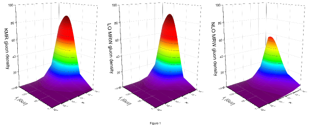
Figure 1: The gluonic $UPDF$ of the $k_{t}$-factorization versus the fractional longitudinal momentum of the parent hadron ($x$) and the transverse momentum of the parton, appearing on the top of the evolution ladder ($k_{t}$) at $\mu=100\;GeV$. The difference in the behavior of the $UPDF$ in different frameworks is a direct consequence of employing different manifestations of the $AOC$ in their respective definitions. To plot these diagrams we have used the $PDF$ libraries of $MMHT2014$ in the $LO$ and the $NLO$ as the input for the equations (5), (7) and (12).

In the figure 1, the $UPDF$ of the $k_{t}$-factorization are plotted against the fractional longitudinal momentum of the parent hadron ($x$) and the transverse momentum of the parton, appearing on the top of the evolution ladder ($k_{t}$). The obvious difference in the behavior of the $UPDF$ in different frameworks is a direct consequence of employing different manifestations of the $AOC$ in their respective definitions.

III The Di-jet production in the p-p collisions at the $LHC$

Generally speaking, the main contributions into the hadronic cross-section of the di-jet productions at the $LHC$, i.e.,

$$P_{1}+P_{2}\to J_{1}+J_{2}+X,$$

are the $LO$ partonic sub-processes:

$$g(\textbf{k}_{1})+g^{*}(\textbf{k}_{2})\to g(\textbf{p}_{1})+g(\textbf{p}_{2}),$$

$$g(\textbf{k}_{1})+g^{*}(\textbf{k}_{2})\to q(\textbf{p}_{1})+\bar{q}(\textbf{p}_{2}),$$

$$q(\textbf{k}_{1})+g^{*}(\textbf{k}_{2})\to q(\textbf{p}_{1})+g(\textbf{p}_{2}).$$ (15)

Since we are considering the forward sector for the partons that are produced in the $k_{t}$-factorization, the stared partons in the equation (15), one can safely neglect the $qq$ and $q\bar{q}$ sub-processes. In the collinear factorization framework, the cross-section of a hadronic $IS$ can be written as a sum over all of the involving partonic cross-sections, times the probability of appearing the particular partonic configuration at top of the evolution ladder of the individual hadrons, i.e.,

$$\sigma_{Hadron-Hadron} =\sum_{a_{1},a_{2}=q,g}\int_{0}^{1}{dx_{1}\over x_{1}}\int_{0}^{1}{dx_{2}\over x_{2}}\;a_{1}(x_{1},\mu_{1}^{2})\;a_{2}(x_{2},\mu_{2}^{2})\;$$

$$\times\hat{\sigma}_{a_{1}-a_{2}}(x_{1},k^{2}_{1,t}=0,\mu_{1}^{2};x_{2},k^{2}_{2,t}=0,\mu_{2}^{2}),$$

(16)

where $\hat{\sigma}_{a_{1}-a_{2}}$ denotes the cross-section of the incoming partons $a_{1}$ and $a_{2}$, respectively with the longitudinal momentum fractions $x_{1}$ and $x_{2}$, the hard scales $\mu_{1}$ and $\mu_{2}$ and neglected transverse momenta. $\hat{\sigma}_{a_{1}-a_{2}}$ may be defined as follows:

$$d\hat{\sigma}_{a_{1}a_{2}}=d\phi_{a_{1}a_{2}}{|{\mathcal{M}_{a_{1}a_{2}}}|^{2}\over F_{a_{1}a_{2}}},$$ (17)

with the multi-particle phase space $d\phi_{a_{1}a_{2}}$,

$$d\phi_{a_{1}a_{2}}\equiv\prod_{i}{d^{3}p_{i}\over 2E_{i}}\delta^{(4)}\left(\sum p_{in}-\sum p_{out}\right),$$ (18)

and the flux factor $F_{a_{1}a_{2}}$,

$$F_{a_{1}a_{2}}\equiv x_{1}x_{2}s.$$ (19)

$s$ is the center of mass energy squared,

$$s=(P_{1}+P_{2})^{2}=2P_{1}.P_{2},$$

with $P_{1}$ and $P_{2}$ being the 4-momenta of the incoming hadrons, where we have neglected the mass of the proton, while working in the infinite momentum frame. ${\mathcal{M}_{a_{1}a_{2}}}$ in the equation (17) are the matrix elements of the partonic sub-processes, the equations (15). To calculate these quantities, one must first understand the exact kinematics that rule over the corresponding partonic sub-processes.

To include the contributions coming from the transverse momentum dependency of the probability functions, one can use the definition of the $UPDF$ in the framework of $k_{t}$-factorization, the equation (2) and rewrite the equation (16) as follows:

$$\sigma_{Hadron-Hadron} =\sum_{a_{1},a_{2}=q,g}\int_{0}^{1}{dx_{1}\over x_{1}}\int_{0}^{1}{dx_{2}\over x_{2}}\int_{0}^{\infty}{dk^{2}_{1,t}\over k^{2}_{1,t}}\int_{0}^{\infty}{dk^{2}_{2,t}\over k^{2}_{2,t}}\;f_{a_{1}}(x_{1},k^{2}_{1,t},\mu_{1}^{2})\;f_{a_{2}}(x_{2},k^{2}_{2,t},\mu_{2}^{2})$$ (20)

$$\times\hat{\sigma}_{a_{1}a_{2}}(x_{1},k^{2}_{1,t},\mu_{1}^{2};x_{2},k^{2}_{2,t},\mu_{2}^{2}).$$

Now, it is convenient to characterize $d\phi_{a_{1}a_{2}}$ in term of the transverse momenta of the product particles, $p_{i,t}$, their rapidities, $y_{i}$, and the azimuthal angles of the emissions, $\varphi_{i}$,

$${d^{3}p_{i}\over 2E_{i}}={\pi\over 2}dp_{i,t}^{2}dy_{i}{d\varphi_{i}\over 2\pi}.$$ (21)

Working in the proton-proton center of mass frame, one may use below kinematics,

$$P_{1} ={\sqrt{s}\over 2}(1,0,0,1),\;\;\;P_{2}={\sqrt{s}\over 2}(1,0,0,-1),$$

$$\textbf{k}_{i} =x_{i}\textbf{P}_{i}+\textbf{k}_{i,\perp},\;\;\;k_{i,\perp}^{2}=-k_{i,t}^{2},\;\;\;i=1,2\;,$$ (22)

where the $k_{i}$ are the 4-momenta of the partons that enter the semi-hard process. Then, for each partonic sub-process, the conservation of the transverse momentum reads as,

$$\textbf{k}_{1,\perp}+\textbf{k}_{2,\perp}=\textbf{p}_{1,\perp}+\textbf{p}_{2,\perp}.$$ (23)

Afterwards, one can simply define,

$$x_{1} ={1\over\sqrt{s}}\left(p_{1,t}e^{+y_{1}}+p_{2,t}e^{+y_{2}}\right),$$

$$x_{2} ={1\over\sqrt{s}}\left(p_{1,t}e^{-y_{1}}+p_{2,t}e^{-y_{2}}\right).$$ (24)

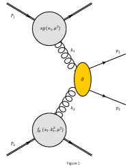
Figure 2: The deep inelastic scattering of two protons in the forward-center configuration. The diagram shows the $g^{*}+g\to q+\bar{q}$ sub-process, assuming that one of the quarks is being produced in the forward sector (bounded by $3.2<|\eta_{f}|<4.7$) and the other in the center sector (bounded by $|\eta_{c}|<2.8$). The parton density related to the first proton is being described with the $integrated$ $PDF$ while the second parton is prepared using the $UPDF$ in one of our presumed frameworks.

The figure 2 illustrates the schematics for a proton-proton deep inelastic collision in the forward-center (or the forward-forward) rapidity sector in a particular partonic sub-process, i.e. $g^{*}+g\to q+\bar{q}$. Working within the boundaries of the forward-center or the forward-forward rapidity sector, without damaging the main assumptions, one can assume that $x_{1}\sim 1$ and $x_{2}\ll 1$. In the direct consequent of a such approximation, we can safely neglect the transverse momentum dependency of the first parton entering the hard process (shift it to the collinear domain), and rewrite the equation (20) as,

$$\sigma_{Hadron-Hadron} =\sum_{a_{1},a_{2}=q,g}\int_{0}^{1}{dx_{1}\over x_{1}}\int_{0}^{1}{dx_{2}\over x_{2}}\int_{0}^{\infty}{dk^{2}_{t}\over k^{2}_{t}}a_{1}(x_{1},\mu_{1}^{2})\;f_{a_{2}}(x_{2},k^{2}_{t},\mu_{2}^{2})$$ (25)

$$\times\hat{\sigma}_{a_{1}a_{2}}(x_{1},\mu_{1}^{2};x_{2},k^{2}_{t},\mu_{2}^{2}),$$

with the $k_{t}$ being defined as,

$$k_{t}=\left[p_{1,t}^{2}+p_{2,t}^{2}+2p_{1,t}p_{2,t}cos(\Delta\varphi)\right]^{1/2},$$ (26)

and $\Delta\varphi=\varphi_{1}-\varphi_{2}$.

After determining the kinematics of the involving processes, it is possible to calculate their matrix elements, i.e. ${\mathcal{M}_{a_{1}a_{2}}}$. To this end, one have to sum over the $dk_{i,t}^{2}/k_{i,t}^{2}$ terms only from the ladder-type diagrams, and somehow systematically dispose the interference (the non-ladder) diagrams, e.g. by using a physical gauge for the gluons,

$$d_{\mu\nu}(k)=-g_{\mu\nu}+{k_{\mu}n_{\nu}+n_{\mu}k_{\nu}\over k.n}.$$ (27)

Note that $n=x_{1}P_{1}+x_{2}P_{2}$ is the gauge-fixing vector. One might expect that neglecting the contributions coming from the non-ladder diagrams, i.e. the diagrams where the production of the jets is a by-product of the hadronic collision (see the reference Modarres9 ; Deak1 ), would have a numerical effect on the results. Hence, using the equation (27) as our choice for the axial gauge for the gluons, we can safely subtract the ”unfactorizable” contributions coming from the non-ladder type diagrams. Thus, using the regular Feynman rules, inserting the ”non-sense” polarization for the incoming gluons

$$\sum\epsilon^{\mu}(\textbf{k}_{i})\epsilon^{*\nu}(\textbf{k}_{i})={k_{i,t}^{\mu}k_{i,t}^{\nu}\over\textbf{k}_{i,t}^{2}},$$ (28)

and imposing the ”eikonal” approximation to justify the use of an on-shell prescription for the off-shell particles (via neglecting the exchanged momenta in the quark-gluon vertices and preserving the spin of the gluons, see the references Modarres9 ; Deak1 ; LIP1 ),

$$-i\bar{u}(p_{i})\gamma^{\mu}u(p_{i})\to{-2i\over k_{i,t}^{2}}P_{i}^{\mu},$$ (29)

one can manage to extract the matrix element, corresponding to the processes of the equation (15), see the appendix A.

Now, using the above equations, one can derive the master equation for the total cross-section of the production of di-jets in the framework of $k_{t}$-factorization,

$$\sigma_{p-p}(P_{1}+P_{2}\to J_{1}+J_{2}) =\sum_{a,c,d=q,g}{1\over 1+\delta_{cd}}\int{p_{1,t}p_{2,t}\over 8\pi^{2}(x_{1}x_{2}s)^{2}}dy_{1}dy_{2}{dp_{1,t}dp_{2,t}\over k^{2}_{t}}d\Delta\varphi\;a(x_{1},\mu^{2})$$ (30)

$$\times\;f_{g}(x_{2},k^{2}_{t},\mu^{2})\;|\mathcal{M}_{a+g\to c+d}(x_{1},\mu^{2};x_{2},k^{2}_{t})|^{2}.$$

The term $1/(1+\delta_{cd})$ restrains the over-counting indices. Note that, the existence of the term $k^{-2}_{t}$ in the equation (30) is the remnant of the re-summation factor, $dk_{t}^{2}/k_{t}^{2}$, from the equation (2) and since we are interested to look for the transverse momentum dependent jets with $p_{i,t}>20\;GeV$, the presence of such denominator would not cause any complication in the master equation. Additionally, we have to decide how to validate our $UPDF$ in the non-perturbative region. i.e. where $k_{t}<\mu_{0}$ with $\mu_{0}=1\;GeV$. A natural option would be to fulfill the requirement that:

$$\lim_{k_{t}^{2}\rightarrow 0}f_{g}(x,k_{t}^{2},\mu^{2})\sim k_{t}^{2},$$

and therefore, one can safely choose the following approximation for the non-perturbative region:

$$f_{g}(x,k_{t}^{2}<\mu_{0}^{2},\mu^{2})={k_{t}^{2}\over\mu_{0}^{2}}g(x,\mu_{0}^{2})T_{g}(\mu_{0}^{2},\mu^{2}).$$ (31)

In the next section, we will introduce some of the numerical methods that have been used for the calculation of the cross-section of the production of di-jets, using the $UPDF$ of $KMR$ and $MRW$.

IV The numerical analysis

We perform the 5-fold integration of the master equation (30), using the $\mathtt{VEGAS}$ algorithm in Monte-Carlo integration. To do this, we have selected the hard-scale of the $UPDF$ as the share of each of the parent hadrons from the total energy of the center-of-mass frame:

$$\mu={1\over 2}E_{CM}.$$ (32)

Variating this normalization value around a factor of 2, will provide each framework with a decent uncertainty bound. One would also set the upper boundaries on the transverse momentum integrations to $p_{i,max}=4\mu$, noting that increasing this upper value does not have any effect on the outcome.

The forward rapidity sectors is conventionally defined as,

$$3.2<|\eta_{f}|<4.8,$$ (33)

where $\eta$ denotes the pseudorapidity of a produced particle,

$$\eta=-ln\left[tan\left({\theta\over 2}\right)\right],$$

with $\theta$ being the angle between the propagation axis and the momentum of the particle. Alternatively, to work in the central rapidity sector, one have to choose,

$$|\eta_{c}|<2.8.$$ (34)

Therefore, while working in the infinite momentum frame i.e. where $\eta\simeq y$, to perform our calculations in the forward-center region, we set:

$$y_{1}=\eta_{c},\;\;\;y_{2}=\eta_{f}.$$

Trivially, the choice

$$y_{1}=\eta_{f},\;\;\;y_{2}=\eta_{f},$$

marks the forward-forward region. Such framework should be ideal to describe the inclusive $CMS$ data regarding the forward-center di-jet measurements for $p_{i,t}>35\;GeV$. After confirming that, one can go further, producing predictions in the framework of forward-forward di-jet production for the $LHC$.

Moreover, as a consequence of employing the inclusive scenario (i.e. $p_{i,t}>35\;GeV$ and limiting the rapidity integrations to the forward or central regions), one must assure that the produced jets must lie within this specific region. Thus, in order to cut-off the collinear and the soft singularities, it is conventional to use the anti-$k_{t}$ algorithm Cacciari , with radius $R=1/2$, bounding the jets to this particular initial setup, through inserting a constraint on the $y-\varphi$ plane:

$$R>\left[(\Delta\varphi)^{2}+(y_{2}-y_{1})^{2}\right]^{1/2}.$$ (35)

Introducing the anti-$k_{t}$ jet constraint ensures the production of 2 separated jets and rejects any single-jet scenarios.

V Results, Discussions and Conclusions

Having in mind the theory and the notions of the previous sections, we are able to calculate the production rates belonging to the di-jets in the forward-center and the forward-forward rapidity sectors, from the perspective of the $k_{t}$-factorization framework, utilizing the $UPDF$ of $KMR$ and $MRW$. The $PDF$ of $Harland-Lang$ et al. MMHT , $MMHT2014$, in the $LO$ and $NLO$ levels, are used as the input functions for the unintegrated gluon densities, i.e., the equations (5), (7) and (12). Additionally, they are fit to be used as the solutions of the $DGLAP$, the $PDF$ of the collinear factorization, directly in the master equation (30). We tend to perform the above calculations in any of our presumed frameworks, the $KMR$, the $LO$ $MRW$ and the $NLO$ $MRW$, then compare the results to each other, to the similar calculations in other frameworks and to the existing experimental data, in the case of the forward-center.

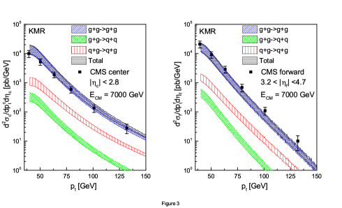
Figure 3: The differential cross-section for the production of di-jets in the forward-center rapidity sector, calculated in the $KMR$ framework for $E_{CM}=7\;TeV$. The contributions from each of the involving sub-processes form the equation (15) have been plotted separately. The black-oblique patterned histograms illustrate the sum of the partonic contributions. To determine the uncertainty of the calculations, we have manipulated the hard scale of the $UPDF$, $\mu=E_{CM}/2$, by a factor of 2. The data point are from the measurements of the $CMS$ collaboration, the reference CMS1 .

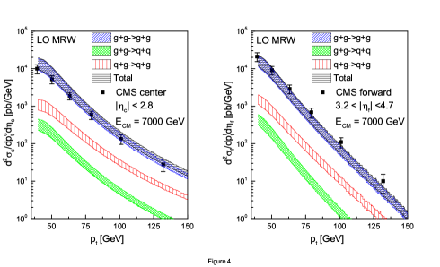
Figure 4: The differential cross-section for the production of di-jets in the forward-center rapidity sector, calculated in the $LO$ $MRW$ framework. The notion of the diagrams are as in the figure 3.

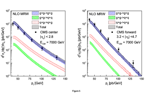
Figure 5: The differential cross-section for the production of di-jets in the forward-center rapidity sector, calculated in the $NLO$ $MRW$ framework. The notion of the diagrams are as in the figure 3.

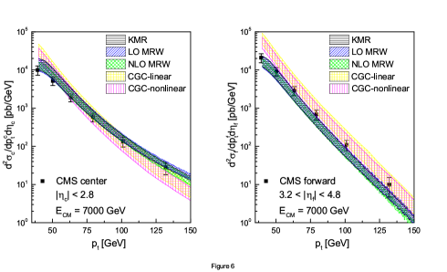
Figure 6: The comparison between the differential cross-sections of the production of di-jets from the forward-center rapidity sector, in the different frameworks of the $k_{t}$-factorization. The results have been prepared as the numerical solutions the equation (30), using the $UPDF$ of $KMR$ and $MRW$ in the $LO$ and $NLO$ with $E_{CM}=7\;TeV$. The data points are from the $CMS$ report CMS1 . The yellow-checkered and the purple-vertically stripped patters represent the calculations in the linear and non-linear $KS$ frameworks, respectively, see the reference kutak1 .

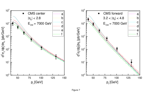
Figure 7: The differential cross-section for the production of di-jets in the forward-center rapidity sector, for different choices of the hard scale and from the dominant $g^{*}+g\to g+g$ sub-process. The calculations have been carried on in the $KMR$ framework for $E_{CM}=7\;TeV$. The histograms $a$ through $f$ have been calculated using the conditions from the equation (36). We have chosen the condition $e$ (the black-continues histograms), i.e. the equation (32), as the primary prescription throughout this work.

So, the figures 3, 4 and 5 present the reader with the differential cross-section for the production of well-separated forward-central di-jets ($d^{2}\sigma/dp_{t}d\eta$), plotted against the transverse momentum of the corresponding jets ($p_{t}$) in the $KMR$, the $LO$ $MRW$ and the $NLO$ $MRW$ schemes respectively. The uncertainty bounds are calculated, variating the hard scale of the $UPDF$ with a factor of 2, since this is the only arbitrary physical parameter in the framework of $k_{t}$-factorization. The blue-hatched pattern, the green-checkered and the red-vertically stripped patterns illustrate the individual contributions of the partonic sub-processes from the equation (15), corresponding to the $g^{*}+g\to g+g$, $g^{*}+g\to q+\bar{q}$ and $g^{*}+q\to g+q$ processes respectively. The black-horizontally stripped pattern represents the sum of the sub-contributions. The calculations have been compared against the experimental data of the $CMS$ collaboration, the reference CMS1 . One immediately notices that the share of the $g^{*}+g\to g+g$ sub-process dominates, relative to the negligible shares of the remaining two sub-processes. Although all of these frameworks are relatively successful in describing the experimental data, see the figure 6, it is interesting to find that the $UPDF$ of $KMR$ do as well as (if not better than) the $UPDF$ of $MRW$ in predicting the experimental results. The closeness of the behavior of different frameworks is a consequence of our choice for the hard scale of the $UPDF$, the equation (32). In order to enlighten this point, the figure 7 illustrates the result of making different choices in such calculations, using the $UPDF$ of the $KMR$. To demonstrate the effect of changing the hard scale of the $UPDF$ in the outcome, the histograms are calculated utilizing the following hard scale prescriptions

$$a)\;\;\;\mu={1\over 2}\left(p_{1,t}+p_{2,t}\right),$$

$$b)\;\;\;\mu={1\over 2}\left(p_{1,t}^{2}+p_{2,t}^{2}\right)^{1/2},$$

$$c)\;\;\;\mu=Max(p_{1,t},p_{2,t}),$$

$$d)\;\;\;\mu={1\over 4}E_{CM},$$

$$e)\;\;\;\mu={1\over 2}E_{CM},$$

$$f)\;\;\;\mu=E_{CM},$$ (36)

where $Max(p_{1,t},p_{2,t})$ returns the higher value between the transverse momenta of the produced jets. To save computation time, we only considered the contributions coming form the dominant $g^{*}+g\to g+g$ sub-processes. The choice $a$, which have been used in the similar calculations (e.g., the references kutak1 ; kutak2 ; kutak3 ; kutak4 ; kutak5 in the high energy factorization, from the point of view of the $UPDF$ of the color gloss condensation, ($CGC$)) proves to be in contrast with the particular manifestation of the $AOC$, specially in the case of $NLO$ $MRW$ $UPDF$. This is in addition to the considerable off-shoot of the results in the smaller values of the transverse momenta belonging to the produced jets. In the figure 6, the yellow-checkered and the purple-vertically stripped patters represent the calculations in the linear and the non-linear $KS$ frameworks, respectively. The above separation between the predictions of the $KS$ framework and the experimental data is apparent. To avoid such complications, we have chosen the condition $e$, in the equation (36), as the primary prescription for the hard scale of our $UPDF$ throughout this work, see the section IV.

Having a closer look into the figure 6, one notices that such off-shooting results also appear in our settings for the production of di-jets. This is perhaps because of the over-simplified dynamics that have been used to derive these measurements. An increase in the precision may be realized via including higher order diagrams and introducing the final state parton showers in this frameworks kutak6 . Beside this point, note that our results show an acceptable agreement with the experimental data of the $CMS$ collaboration, reference CMS1 . Another interesting observation is that in the large $k_{t}$, where the higher order corrections become important, the calculations in the $KMR$ approach start to separate from the $LO\;MRW$ and behave similar to the $NLO\;MRW$. The reason is that the inclusion of the $non-diagonal$ splitting functions into the domain of the $AOC$ introduces some corrections from the $NLO$ region (in the form of $ln(1/x)$ re-summations) into the $KMR$ formalism.

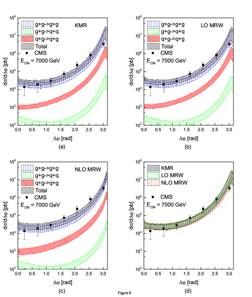
Figure 8: The differential cross-section for the production of di-jets versus the angle of the out-coming jets, $\Delta\varphi$. The calculations are in the forward-center rapidity sector for $E_{CM}=7\;TeV$. The panels (a), (b) and (c) illustrate the calculations, utilizing the $UPDF$ of $KMR$, $LO$ $MRW$ and $NLO$ $MRW$, respectively. The contributions from each of the involving sub-processes are shown separately. The panel (d) presents the comparison of these measurements against each other as well as the experimental data of the $CMS$ collaboration, the reference CMS2 . The uncertainty of the calculations are provided through manipulating the hard scale of the $UPDF$ by a factor of 2.

A recent report from the $CMS$ collaboration, the reference CMS2 , concerns the angular distribution of the produced jets in the forward-center rapidity sector from a deep inelastic event at the $LHC$. Making use of this new information, we have calculated the differential cross-section of the forward-central di-jet production ($d\sigma/d\Delta\varphi$), plotted in the figure 8 against the angular difference of the produced partons (or equivalently the angular difference of the produced jets, $\Delta\varphi$). The panels (a), (b) and (c) in this figure illustrate the details of the calculations in each framework, consisting of the individual contributions of the sub-processes and the corresponding uncertainty bounds. The panel (d) presents the reader with the comparison of the total amounts in the presumed formalisms to each other and to the data from the reference CMS2 . Again, the results in the $KMR$ approach seems to be equally good (or better than) those from the $MRW$ in the $LO$ or the $NLO$.

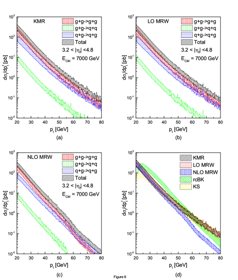
Figure 9: The calculated predictions for the production of forward-forward di-jets in the framework of $k_{t}$-factorization with the central-mass energy of $7\;TeV$. The differential cross-section for the production of di-jets are plotted against the transverse momenta of the produced jets, in the $KMR$, $LO\;MRW$ and $NLO\;MRW$ schemes (i.e. the panels (a), (b) and (c), respectively), demonstrating the contributions of the individual sub-processes. The uncertainty bound is determined by manipulating the hard scale of the $UPDF$, $\mu=E_{CM}/2$, by a factor of 2. The panel (d) represents a comparison between the results of the $k_{t}$-factorization with the results from other frameworks, namely the Balitsky-Kovchegov $TMD$ $PDF$ convoluted with running coupling corrections ($rcBK$, see the references BK1 ; BK2 ) and the Kutak-Sapeta $TMD$ $PDF$ ($KS$), reference kutak5 .

After proving the success of our formalism in describing the experimental data for the production of di-jets in the forward-center rapidity region, we can move forward with the prediction of a similar event, in the forward-forward sector, i.e. by choosing the rapidity of the produced jets ($y_{1}$ and $y_{2}$) to be both in the boundaries that where specified within the equation (33). Therefore, in the figure 9 the reader is presented with our predictions regarding the dependency of the differential cross-section of the forward-forward di-jet production ($d\sigma_{f}/dp_{t}^{f}$) to the transverse momenta of the produced jets ($p_{t}$), in the framework of $k_{t}$-factorization. The panels (a), (b) and (c) of the figure illustrate these predictions in the $KMR$, the $LO\;MRW$ and the $NLO\;MRW$ formalisms, respectively. The contributions of the individual partonic sub-processes are included. These contributions have the same general behavior as in the forward-central case, in spite of the fact that the measured contribution for the $g^{*}+g\to g+g$ and the $g^{*}+q\to g+q$ sub-processes are closer, compared to their counterparts from the forward-center region,

$$\hat{\sigma}_{F-C}(g^{*}+g\to g+g)\gg\hat{\sigma}_{F-C}(g^{*}+q\to g+q)\gg\hat{\sigma}_{F-C}(g^{*}+g\to q+\bar{q}),$$

$$\hat{\sigma}_{F-F}(g^{*}+g\to g+g)\gtrsim\hat{\sigma}_{F-F}(g^{*}+q\to g+q)\gg\hat{\sigma}_{F-F}(g^{*}+g\to q+\bar{q}).$$ (37)

In addition, one can clearly perceive the effect of the $\Theta(1-z-(k_{t}^{2}/\mu^{2}))$ constraint in the $NLO\;MRW$ results, causing a steep descend in the corresponding histograms, in contrast with the behaviors of the results of the $KMR$ and the $LO\;MRW$ formalisms. Again, the similarity of the predictions of the $KMR$ and the $LO\;MRW$ schemes are a consequence of our choice of the hard scale, $\mu$. Such similarity was also observed else where, e.g. the references Modarres7 ; Modarres8 ; Modarres9 , specially in the smaller $x$ domains.

The panel (d) of the figure 9 represents a comparison between the results of the $k_{t}$-factorization with the results from other frameworks, namely the $Balitsky$-$Kovchegov$ $TMD$ $PDF$ convoluted with the running coupling corrections ($rcBK$, see the references BK1 ; BK2 ) and the $Kutak$-$Sapeta$ $TMD$ $PDF$ ($KS$), the reference kutak5 . Both of these frameworks are specially designed to describe the behavior of the small-x region, incorporating the non-linear evolution of the $unintegrated$ parton densities with the $KS$ framework and the high energy factorization ($HEF$) formalism, in accordance with the $BFKL$ iterative evolution equation. In the absence of any experimental data, we refrain ourselves from any assessments regarding these results. Nevertheless, the predictions of the $KMR$ scheme (because of its previous success) may provide a base line for a sound comparison. Also, the singular behavior of the $NLO\;MRW$ results may appear undesirable.

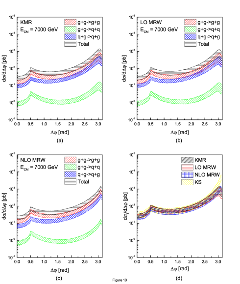
Figure 10: The calculated predictions regarding the dependency of the differential cross-section for the production of forward-forward di-jets to $\Delta\varphi$ using the $UPDF$ of $k_{t}$-factorization for $E_{CM}=7\;TeV$. The notion on the diagrams are as in the figure 9. In the panel (d), we have compared our results with the predictions made using the $KS$ $TMD$ $PDF$ from the reference kutak5 .

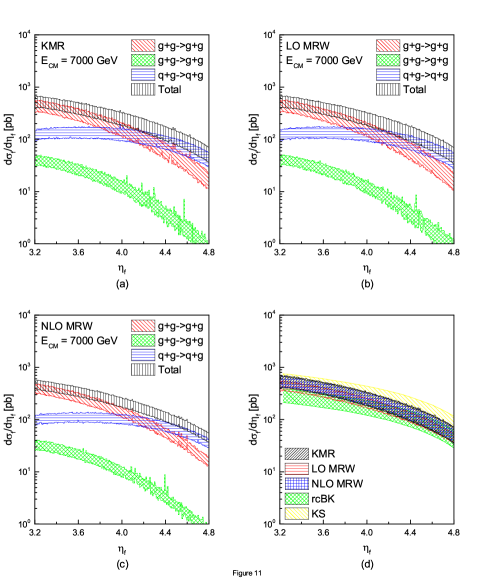
Figure 11: The calculated predictions regarding the dependency of the differential cross-section for the production of forward-forward di-jets to rapidity of the produced jets, using the $UPDF$ of $k_{t}$-factorization for $E_{CM}=7\;TeV$. The notion on the diagrams are as in the figure 9. In the panel (d), we have compared our results with the predictions made using the $rcBK$ and $KS$ $TMD$ $PDF$ from the reference kutak5 .

Similar predictions are presented in the figures 10 and 11, describing the dependency of the differential cross-section of the forward-forward di-jet production, to the angle of the produced jets ($d\sigma_{f}/d\Delta\varphi$ to $\Delta\varphi$ in the figure 10) and to their rapidity ($d\sigma_{f}/d\eta_{f}$ to $\eta_{f}$ in the figure 11). The notions of these diagrams are as in the figure 9. The panel (d) of each figure includes the comparison of the $k_{t}$-factorization results to the existing results in the $rcBK$ and the $KS$ frameworks. The irregular behavior of the $NLO\;MRW$ scheme in both cases, manifests itself in the form of lower values of the predicted differential cross-section. Again, the reliability of these predictions lies within the excellent credit of the $KMR$ $UPDF$ in describing the high energy $QCD$ events.

In summary, throughout this work, we have tested the $UPDF$ of the $k_{t}$-factorization, namely the $KMR$ and $MRW$ formalisms in the $LO$ and the $NLO$, calculating the production rate of the di-jet pairs at the deep inelastic $QCD$ collisions in the forward-center rapidity sector, compared the results to the existing experimental data of the $CMS$ collaborations and to the results of other frameworks. Through our analysis we have suggested that despite the theoretical advantages of the $MRW$ formalism, the $KMR$ approach performs as good as (if not better) behavior toward describing the experimental data. This is in general agreement with our previous findings, the references Modarres1 ; Modarres2 ; Modarres3 ; Modarres4 ; Modarres5 ; Modarres6 ; Modarres7 ; Modarres8 ; Modarres9 . Additionally, one can clearly see that the $KMR$ or $MRW$ prescription work better than the $KS$ in describing the experiment. Based on these observations one concludes that the hard-scale dependence should be necessarily included in $TMD$ analysis. Furthermore, we have predicted the results of the similar events in the forward-forward rapidity region, relying on the previous success of the $UPDF$ of the $k_{t}$-factorization.

Appendix A The matrix elements of the partonic sub-processes

Assuming that $\mu_{1}=\mu_{2}\equiv\mu$, the matrix element squares, $|\mathcal{M}_{a_{1}+a_{2}\to b_{1}+b_{2}}|^{2}$, corresponding to the equations (15) can be defined for a $QCD$ $IS$ event as follows (also see the reference kutak5 )

$$|\mathcal{M}_{g+g\to g+g}(x_{1},\mu;x_{2},k^{2}_{t})|^{2} =C_{1}A_{1},$$

$$|\mathcal{M}_{g+g\to q+\bar{q}}(x_{1},\mu;x_{2},k^{2}_{t})|^{2} =C_{2}A_{2}+C^{\prime}_{2}A^{\prime}_{2},$$

$$|\mathcal{M}_{q+g\to q+g}(x_{1},\mu;x_{2},k^{2}_{t})|^{2} =C_{3}A_{3}+C^{\prime}_{3}A^{\prime}_{3},$$ (38)

with

$$C_{1} ={9\over 8}\left({\alpha_{S}(\mu^{2})\over 4\pi}\right)^{2}$$

$$C_{2} ={1\over 6}\left({\alpha_{S}(\mu^{2})\over 4\pi}\right)^{2}\;\;\;,C^{\prime}_{2}={1\over 8}C_{2},$$

$$C_{3} ={4\over 9}\left({\alpha_{S}(\mu^{2})\over 4\pi}\right)^{2}\;\;\;,C^{\prime}_{3}={1\over 8}C_{3},$$ (39)

and

$$A_{1} ={2(e^{\Delta y}R_{t}+1)^{2}(R_{t}e^{-\Delta y}(R_{t}e^{-\Delta y}+1)+1)^{2}(cos(\Delta\varphi)+2cosh(\Delta y))\over R_{t}^{2}(R_{t}e^{-\Delta y}+1)^{2}(cos(\Delta\varphi)+cosh(\Delta y))},$$

$$A_{2} ={(R_{t}+e^{-\Delta y})^{2}(R_{t}^{2}e^{-\Delta y}+e^{\Delta y})\over R_{t}(R_{t}e^{-\Delta y}+1)^{2}},$$

$$A^{\prime}_{2} ={(R_{t}+e^{-\Delta y})^{2}(R_{t}^{2}e^{-\Delta y}+e^{\Delta y})\over R_{t}(R_{t}e^{-\Delta y}+1)^{2}(cosh(\Delta y)-cos(\Delta\varphi))}cos(\Delta\varphi),$$

$$A_{3} ={(R_{t}+e^{-\Delta y})^{2}((R_{t}+e^{\Delta y})^{2}+R_{t}^{2})\over 2R_{t}(R_{t}e^{-\Delta y}+1)(cosh(\Delta y)-cos(\Delta\varphi))},$$

$$A^{\prime}_{3} =2e^{-\Delta y}(e^{-\Delta y}-cos(\Delta\varphi)){(R_{t}+e^{-\Delta y})^{2}((R_{t}+e^{\Delta y})^{2}+R_{t}^{2})\over 2R_{t}(R_{t}e^{-\Delta y}+1)(cosh(\Delta y)-cos(\Delta\varphi))},$$ (40)

where

$$\Delta y=y_{2}-y_{1},\;\;\;R_{t}={p_{1,t}\over p_{2,t}}.$$

Using the above information, one can calculate the cross-sections of the equation (15).

References

- (1) V.N. Gribov and L.N. Lipatov, Yad. Fiz., 15 (1972) 781.
- (2) L.N. Lipatov, Sov.J.Nucl.Phys., 20 (1975) 94.
- (3) G. Altarelli and G. Parisi, Nucl.Phys.B, 126 (1977) 298.
- (4) Y.L. Dokshitzer, Sov.Phys.JETP, 46 (1977) 641.
- (5) L.V. Gribov, E.M. Levin, M.G. Ryskin, Phys. Rep. 100, (1983) 1.
- (6) E.M. Levin, M.G. Ryskin, Yu.M. Shabelsky, A.G. Shuvaev, Sov. J. Nucl. Phys. 53, (1991) 657.
- (7) S. Catani,M. Ciafaloni, F. Hautmann, Phys. Lett. B 242, (1990) 97.
- (8) S. Catani, M. Ciafoloni, F. Hautmann, Nucl. Phys. B 366, (1991) 135.
- (9) J.C. Collins, R.K. Ellis, Nucl. Phys. B 360, (1991) 3.
- (10) G. Watt, A.D. Martin and M.G. Ryskin, Eur.Phys.J.C 31 (2003) 73.
- (11) M.A. Kimber, A.D. Martin and M.G. Ryskin, Phys.Rev.D, 63 (2001) 114027.
- (12) A.D. Martin, M.G. Ryskin, G. Watt, Eur.Phys.J.C, 66 (2010) 163.
- (13) M.A. Kimber, J. Kwiecinski, A.D. Martin, A.M. Stasto, Phys.Rev.D 62, (2000) 094006.
- (14) M.A. Kimber, Unintegrated Parton Distributions, Ph.D. Thesis, University of Durham, U.K. (2001).
- (15) G. Watt, A.D. Martin and M.G. Ryskin, Phys.Rev.D 70 (2004) 014012.
- (16) M. Ciafaloni, Nucl.Phys.B, 296 (1988) 49.
- (17) S. Catani, F. Fiorani, and G. Marchesini, Phys.Lett.B, 234 (1990) 339.
- (18) S. Catani, F. Fiorani, and G. Marchesini, Nucl.Phys.B, 336 (1990) 18.
- (19) M. G. Marchesini, Proceedings of the Workshop QCD at 200 TeV Erice, Italy, edited by L. Cifarelli and Yu.L. Dokshitzer, Plenum, New York (1992) 183.
- (20) G. Marchesini, Nucl.Phys.B, 445 (1995) 49.
- (21) V.S. Fadin, E.A. Kuraev and L.N. Lipatov, Phys. Lett. B, 60 (1975) 50.
- (22) L.N. Lipatov, Sov.J.Nucl.Phys., 23 (1976) 642.
- (23) E.A. Kuraev, L.N. Lipatov and V.S. Fadin, Sov. Phys. JETP, 44 (1976) 45.
- (24) E.A. Kuraev, L.N. Lipatov and V.S. Fadin, Sov. Phys. JETP, 45 (1977) 199.
- (25) Ya.Ya. Balitsky and L.N. Lipatov, Sov.J.Nucl.Phys., 28 (1978) 822.
- (26) J. Kwiecinski, A.D. Martin, P.J. Sutton, Phys. Rev. D 52 (1995) 1445.
- (27) H. Jung, Comput. Phys. Commun. 143 (2002) 100-111.
- (28) H. Jung et al, Eur. Phys. J. C70 (2010) 1237-1249.
- (29) F. Hautmann, M. Hentschinski, H. Jung, arXiv:1207.6420 [hep-ph].
- (30) F. Hautmann, H. Jung, S. Taheri Monfared, Eur.Phys.J. C74 (2014) 3082.
- (31) O. Gituliar, M. Hentschinski, K. Kutak, JHEP 1601 (2016) 181.
- (32) M. Modarres, H. Hosseinkhani, Nucl.Phys.A, 815 (2009) 40.
- (33) M. Modarres, H. Hosseinkhani, Few-Body Syst., 47 (2010) 237.
- (34) H. Hosseinkhani, M. Modarres, Phys.Lett.B, 694 (2011) 355.
- (35) H. Hosseinkhani, M. Modarres, Phys.Lett.B, 708 (2012) 75.
- (36) M. Modarres, H. Hosseinkhani, N. Olanj, Nucl.Phys.A, 902 (2013) 21.
- (37) M. Modarres, H. Hosseinkhani and N. Olanj, Phys.Rev.D, 89 (2014) 034015.
- (38) M. Modarres, H. Hosseinkhani, N. Olanj and M.R. Masouminia, Eur. Phys. J. C 75 (2015) 556.
- (39) M. Modarres, M.R. Masouminia, H. Hosseinkhani, and N. Olanj, Nucl. Phys. A 945 (2016) 168.
- (40) M. Modarres, M.R. Masouminia, R. Aminzadeh Nik, H. Hosseinkhani, N. Olanj, Phys.Rev.D, 94 (2016) 0744035.
- (41) K. Kutak and J. Kwiecinski, Eur. Phys. J. C 29 (2003) 521 [arXiv:hep-ph/0303209].
- (42) M. Deak, F. Hautmann, H. Jung and K. Kutak, arXiv:1012.6037 [hep-ph].
- (43) K, Kutak, S, Sapeta, Phys. Rev. D 86 (2012) 094043.
- (44) M. Deak, F. Hautmann, H. Jung, K. Kutak, JHEP 0909 (2009) 121.
- (45) A. van Hameren, P. Kotko, K. Kutak, S. Sapeta, arXiv:1404.6204v2 [hep-ph].
- (46) CMS Collaboration, CMS-PAS-FSQ-12-008, (2014).
- (47) CMS Collaboration, CMS-PAS-FWD-10-006, (2011).
- (48) L. A. Harland-Lang, A. D. Martin, P. Motylinski, R.S. Thorne, Eur.Phys.J.C 75 (2015) 204.
- (49) J. Kwiecinski, A.D. Martin and A.M. Stasto, Phys.Rev.D, 56 (1997) 3991.
- (50) K. Golec-Biernat and A.M. Stasto, Phys.Rev.D, 80 (2009) 014006.
- (51) M.A. Kimber, A.D. Martin and M.G. Ryskin, Eur. Phys. J. C12 (2000) 655.
- (52) G. Watt, Parton Distributions, Ph.D. Thesis, University of Durham, U.K. (2004).
- (53) W. Furmanski, R. Petronzio, Phys. Lett. B 97, 437 (1980).
- (54) M. Deak, Transversal momentum of the electroweak gauge boson and forward jets in high energy factorisation at the , Ph.D. Thesis, University of Hamburg, Germany, 2009.
- (55) S. P. Baranov, A.V. Lipatov, and N. P. Zotov, Phys. Rev. D 78 (2008) 014025.
- (56) M. Cacciari, G. P. Salam and G. Soyez, JHEP 0804 (2008) 063.
- (57) M. Bury, M. Deak, K. Kutak and S. Sapeta, arXiv:1604.01305 [hep-ph].
- (58) I. Balitsky, Nucl. Phys. B 463 (1996) 99.
- (59) Y. V. Kovchegov, Phys. Rev. D 60 (1999) 034008.