A study on nonnegativity preservation in finite element approximation of Nagumo-type nonlinear differential equations

Abstract

Preservation of nonnengativity and boundedness in the finite element solution of Nagumo-type equations with general anisotropic diffusion is studied. Linear finite elements and the backward Euler scheme are used for the spatial and temporal discretization, respectively. An explicit, an implicit, and two hybrid explicit-implicit treatments for the nonlinear reaction term are considered. Conditions for the mesh and the time step size are developed for the numerical solution to preserve nonnegativity and boundedness. The effects of lumping of the mass matrix and the reaction term are also discussed. The analysis shows that the nonlinear reaction term has significant effects on the conditions for both the mesh and the time step size. Numerical examples are given to demonstrate the theoretical findings.

AMS 2010 Mathematics Subject Classification. 65M60, 65M50

Key words. finite element method, anisotropic diffusion, nonnegativity preservation, boundedness preservation, maximum principle

1 Introduction

We consider Nagumo-type equations in the form

$$\frac{\partial u}{\partial t}-\nabla\cdot(\mathbb{D}\nabla u)=uf(u),\quad\text{ in }\quad\Omega_{T}=\Omega\times(0,T]$$ (1)

$$u(\mbox{\boldmath$x$},t)=g(\mbox{\boldmath$x$},t),\qquad\qquad\quad\text{ on }\quad\partial\Omega\times(0,T]$$ (2)

$$u(\mbox{\boldmath$x$},0)=u_{0}(\mbox{\boldmath$x$}),\qquad\qquad\quad\text{\, in }\quad\Omega$$ (3)

where $\Omega\subset\mathbb{R}^{d}$ is a connected, bounded polygonal or polyhedral domain ($d=1,2$ or $3$ is the space dimension), $\mbox{\boldmath$x$}=(x_{1},\cdots,x_{d})^{T}$ denotes the coordinates on $\Omega$, $T>0$ is a fixed time, $f(u)$, $g(\mbox{\boldmath$x$},t)$, and $u_{0}(\mbox{\boldmath$x$})$ are given functions, and $\mathbb{D}$ denotes the diffusion tensor that can be isotropic (when it is in the form of $\mathbb{D}=\alpha I$, with $\alpha$ being a scalar function and $I$ being the identity matrix) or anisotropic. We assume that $\mathbb{D}$ is continuous and symmetric and uniformly positive definite on $\Omega$. In our analysis, $f(u)$ and $f^{\prime}(u)$ are assumed to be continuous and bounded for all bounded $u$. A special example is the well-known Nagumo equation [34, 36] where $f(u)=(1-u)(u-a)$ and $a\in(0,1)$ is a parameter. It can be shown (using an argument similar to the proof of the maiximum principle for linear parabolic equations [13]) that the solution of the problem (1), (2), and (3) is nonnegative when $g$ and $u_{0}$ are nonnegative. Moreover, for the case of the Nagumo equation where $f(1)=0$, we have the boundedness $u\leq 1$ when $g\leq 1$ and $u_{0}\leq 1$.

Nagumo-type equations arise in various fields including physiology, biological and chemical processes, and ecology; e.g., see [2, 18, 24, 27, 33, 40, 42, 44, 45]. The Nagumo equation also appears as one of the two coupled equations in the well-known Fitzhugh-Nagumo model [12, 17, 19, 25, 30]. Understanding the former will help with understanding the latter. The numerical solution of Nagumo-type equations and corresponding models has been studied extensively in the past; e.g., see [1, 7, 11, 12, 20, 22, 26, 30, 34, 39, 41]. However, very little attention has so far been paid to the studies of preservation of solution nonnegativity and boundedness in the discretization of Nagumo-type equations. The existing work includes [7, 32, 39, 41] where only finite difference discretization and isotropic diffusion have been considered. On the other hand, preservation of solution nonnegativity and boundedness has important physical implications and has attracted considerable attention from researchers in the recent years [7, 14, 15, 16, 28, 29, 31, 38, 43, 46, 47]. For example, Li and Huang [28, 29] have developed conditions for general linear diffusion equations for the linear finite element solution to satisfy maximum principle (MP). The schemes in [38, 46] (finite volume methods) and [47] (discontinuous Galerkin schemes) can be used for nonlinear equations but only allow a small time step due to their explicit time integration.

The objective of this work is to study preservation of solution nonnengativity and boundedness in the finite element approximation of Nagumo-type equations with general anisotropic diffusion. We consider anisotropic diffusion here because Nagumo-type equations with anisotropic diffusion can arise from various applications. For example, in cardiac electrophysiology, the conductivity tensor varies with location and direction. The typical conductivities in cardiac tissue are 0.05 m/s for the sinoatrial and the atrioventricular node, 1 m/s for the atrial pathways, the His bundle and the ventricular muscle bundle, and 4 m/s in the Purkinje fibers [18]. In chemical systems with excitable and oscillatory media, the diffusion tensor is also heterogeneous and anisotropic [35]. We shall use linear finite elements and the backward Euler scheme for the spatial and temporal discretization, respectively. Four treatments of the nonlinear reaction term will be considered, including an explicit, an implicit, and two hybrid explicit-implicit treatments. Conditions for the mesh and the time step size will be developed for the numerical solution to preserve nonnegativity and boundedness. The effects of lumping of the mass matrix and the reaction term will also be discussed. It is emphasized that the current work is a nontrivial extension of our previous work [29] where only linear diffusion equations have been studied. As will be seen, the nonlinear reaction term can have significant effects on the mesh and time step size conditions.

The rest of the paper is organized as follows. Sect. 2 introduces the finite element formulation for (1). Conditions for nonnegativity preservation using different treatments of Nagumo nonlinearity are developed in Sect. 3. Lumping for the mass matrix and the reaction term is discussed in Sect. 4, followed by the investigation of boundedness preservation in Sect. 5. Numerical results are presented in Sect. 6, and conclusions are drawn in Sect. 7.

2 Finite element formulation

In this section we describe the linear finite element approximation of the Nagumo-type equation (1). Assume that an affine family of simplicial triangulations $\{\mathcal{T}_{h}\}$ is given for $\Omega$. Define

$$U_{g}=\{v\in H^{1}(\Omega),\quad v|_{\partial\Omega}=g\}.$$

Let $g_{h}$ be a piecewise linear approximation of $g$ on $\mathcal{T}_{h}$. We denote the linear finite element space associated with $\mathcal{T}_{h}$ and $g_{h}$ by $U^{h}_{g_{h}}$. A linear finite element solution $u_{h}(t)\in U^{h}_{g_{h}},\;t\in(0,T]$ for (1) is defined by

$$\int_{\Omega}\frac{\partial u_{h}}{\partial t}\,v_{h}d\mbox{\boldmath$x$}+\int_{\Omega}(\nabla v_{h})^{T}\;\mathbb{D}\nabla u_{h}d\mbox{\boldmath$x$}=\int_{\Omega}u_{h}f(u_{h})\,v_{h}d\mbox{\boldmath$x$},\quad\forall v_{h}\in U_{0}^{h}$$ (4)

where $U_{0}^{h}$ is the subspace of the linear finite element space with vanishing boundary values.

The above equation can be cast in matrix form. Denote the numbers of the elements, vertices, and interior vertices of $\mathcal{T}_{h}$ by $N_{e}$, $N_{v}$, and $N_{vi}$, respectively. For notational simplicity, we assume that the vertices have been ordered in such a way that the first $N_{vi}$ vertices are the interior vertices. Let $\phi_{j}$ be the linear basis function associated with the $j$-th vertex, $\mbox{\boldmath$x$}_{j}$. Then we can express $u_{h}$ as

$$u_{h}=\sum_{j=1}^{N_{v}}u_{j}\phi_{j}.$$ (5)

Inserting this into (4) and taking $v_{h}=\phi_{i}$ ($i=1,...,N_{vi}$) successively, we obtain the matrix form of the semi-discrete system as

$$M\,\frac{d\mbox{\boldmath$u$}}{dt}+A\,\mbox{\boldmath$u$}=\mbox{\boldmath$b$}(u_{h})+\mbox{\boldmath$g$},$$ (6)

where $\mbox{\boldmath$u$}=(u_{1},...,u_{N_{vi}},u_{N_{vi}+1},...,u_{N_{v}})^{T}$ is the unknown vector and $M$ and $A$ are the mass and stiffness matrices, respectively. The entries of the matrices are given by

$$m_{ij}=\begin{cases}\int_{\Omega}\phi_{j}\phi_{i}\,d\mbox{\boldmath$x$}=\sum\limits_{K\in\mathcal{T}_{h}}\int_{K}\phi_{j}\phi_{i}\,d\mbox{\boldmath$x$},&i=1,...,N_{vi}\\ 0,&i=N_{vi}+1,...,N_{v}\end{cases}$$ (7)

$$a_{ij}=\begin{cases}\int_{\Omega}(\nabla\phi_{i})^{T}\;\mathbb{D}\nabla\phi_{j}\,d\mbox{\boldmath$x$}=\sum\limits_{K\in\mathcal{T}_{h}}|K|(\nabla\phi_{i})^{T}\;\mathbb{D}_{K}\nabla\phi_{j},&i=1,...,N_{vi}\\ \delta_{ij},&i=N_{vi}+1,...,N_{v}\end{cases}$$ (8)

where $j=1,...,N_{v}$, $\mathbb{D}_{K}$ is the average of $\mathbb{D}$ over $K$, and $|K|$ denotes the volume of $K$. The right-hand side vectors $\mbox{\boldmath$b$}(u_{h})=(b_{i})$ and $\mbox{\boldmath$g$}=(g_{i})$ are given by

$$b_{i}=\begin{cases}\int_{\Omega}u_{h}f(u_{h})\phi_{i}\,d\mbox{\boldmath$x$}=\sum\limits_{K\in\mathcal{T}_{h}}\int_{K}u_{h}f(u_{h})\phi_{i}\,d\mbox{\boldmath$x$},&i=1,...,N_{vi}\\ 0,&i=N_{vi}+1,...,N_{v}\end{cases}$$ (9)

$$g_{i}=\begin{cases}0,&i=1,...,N_{vi}\\ g(\mbox{\boldmath$x$}_{i},t),&i=N_{vi}+1,...,N_{v}.\end{cases}$$ (10)

For the time discretization we denote the numerical approximation of the solution at $t=t_{n}$ by $u_{h}^{n}$. Applying the backward Euler method to all but the reaction term in (6), we get

$$M\,\frac{\mbox{\boldmath$u$}^{n+1}-\mbox{\boldmath$u$}^{n}}{\Delta t_{n}}+A\,\mbox{\boldmath$u$}^{n+1}=\mbox{\boldmath$\tilde{b}$}(\mbox{\boldmath$u$}^{n},\mbox{\boldmath$u$}^{n+1})+\mbox{\boldmath$g$}^{n+1},$$ (11)

where $\Delta t_{n}=t_{n+1}-t_{n}$, $\mbox{\boldmath$g$}^{n+1}=\mbox{\boldmath$g$}(t_{n+1})$, and $\mbox{\boldmath$\tilde{b}$}(\mbox{\boldmath$u$}^{n},\mbox{\boldmath$u$}^{n+1})$ is an approximation of $\mbox{\boldmath$b$}(u_{h})$ for the time step.

We investigate four approximations in the current work. The first one (called the explicit method or EM) is to define $\mbox{\boldmath$\tilde{b}$}(\mbox{\boldmath$u$}^{n},\mbox{\boldmath$u$}^{n+1})=\mbox{\boldmath$b$}(u_{h}^{n})$. This explicit treatment has been commonly used in the so-called implicit-explicit integration of semi-linear parabolic equations; e.g., see [3, 4, 10, 23]. The second approximation is a fully implicit method (IM) that treats the product implicitly, i.e., $\mbox{\boldmath$\tilde{b}$}(\mbox{\boldmath$u$}^{n},\mbox{\boldmath$u$}^{n+1})=\mbox{\boldmath$b$}(u_{h}^{n+1})$. The third and last approximations are hybrid explicit-implicit methods (HEIM) that use an explicit treatment for some factors and implicit treatment for others in the product. The detail of these approximations and their effects on the preservation of nonnegativity and boundedness of the solution will be discussed in the next section.

3 Preservation of nonnegativity

In this section we describe four approximations of the reaction term and study the conditions on the mesh and the time step under which the numerical solution of the system (6) preserves the nonnegativity of the solution of the continuous problem. We assume that $f(u)$ and $f^{\prime}(u)$ exist and are continuous and bounded for any bounded $u\in\mathbb{R}$.

3.1 Dihedral angles and nonobtuse angle conditions

Consider a generic element $K\in\mathcal{T}_{h}$ and denote its vertices by $\mbox{\boldmath$x$}_{0},\,...,\,\mbox{\boldmath$x$}_{d}$. Note that it is more proper to denote these vertices by $\mbox{\boldmath$x$}_{0}^{K},\,...,\,\mbox{\boldmath$x$}_{d}^{K}$. For notational simplicity we suppress the superscript $K$ as long as no confusion is caused. This convention will apply to other related quantities. Define the edge matrix (of size $d\times d$) of $K$ as

$$E=[\mbox{\boldmath$x$}_{1}-\mbox{\boldmath$x$}_{0},\cdots,\mbox{\boldmath$x$}_{d}-\mbox{\boldmath$x$}_{0}].$$ (12)

Notice that $E$ is non-singular as long as $K$ is not degenerate. Using the edge matrix we can define the so-called $q$-vectors as

$$[\mbox{\boldmath$q$}_{1},\cdots,\mbox{\boldmath$q$}_{d}]=E^{-T},\quad\mbox{\boldmath$q$}_{0}=-\sum_{i=1}^{d}\mbox{\boldmath$q$}_{i}.$$ (13)

Denote the face opposite to vertex $\mbox{\boldmath$x$}_{i}$ (i.e., the face not having $\mbox{\boldmath$x$}_{i}$ as its vertex) by $S_{i}$.

      Lemma 3.1.

The vector $\mbox{\boldmath$q$}_{i}$ is normal to the face $S_{i}$ for $i=0,1,\cdots,d$.

Proof.

For $i=1,\cdots,d$, from the definition (13) we have

$$\mbox{\boldmath$q$}_{i}^{T}(\mbox{\boldmath$x$}_{j}-\mbox{\boldmath$x$}_{0})=\delta_{ij},\quad j=1,...,d$$

which implies that $\mbox{\boldmath$q$}_{i}$ is orthogonal to $(d-1)$ edges of $S_{i}$ and therefore orthogonal to $S_{i}$ itself. For $\mbox{\boldmath$q$}_{0}$, we have, for $i,j=1,...,d$,

$$\mbox{\boldmath$q$}_{0}^{T}(\mbox{\boldmath$x$}_{i}-\mbox{\boldmath$x$}_{j}) = \mbox{\boldmath$q$}_{0}^{T}(\mbox{\boldmath$x$}_{i}-\mbox{\boldmath$x$}_{0})-\mbox{\boldmath$q$}_{0}^{T}(\mbox{\boldmath$x$}_{j}-\mbox{\boldmath$x$}_{0})$$

$$= -\sum_{k=1}^{d}\mbox{\boldmath$q$}_{k}^{T}(\mbox{\boldmath$x$}_{i}-\mbox{\boldmath$x$}_{0})+\sum_{k=1}^{d}\mbox{\boldmath$q$}_{k}^{T}(\mbox{\boldmath$x$}_{j}-\mbox{\boldmath$x$}_{0})$$

$$= -\sum_{k=1}^{d}\delta_{ki}+\sum_{k=1}^{d}\delta_{kj}=-1+1=0,$$

which implies that $\mbox{\boldmath$q$}_{0}$ is orthogonal to $S_{0}$. ∎

      Lemma 3.2.

The vector $\mbox{\boldmath$q$}_{i}$ is equal to the gradient of the linear basis function at $\mbox{\boldmath$x$}_{i}$, i.e., $\mbox{\boldmath$q$}_{i}=\nabla\phi_{i}$, for $i=0,1,\cdots,d$.

Proof.

We first prove for the result for $i=1,\cdots,d$. From the definition of the linear basis functions, we have

$$\sum_{i=0}^{d}\phi_{i}=1,\qquad\sum_{i=0}^{d}\phi_{i}\mbox{\boldmath$x$}_{i}=\mbox{\boldmath$x$}.$$

Combining them we get

$$\sum_{i=1}^{d}(\mbox{\boldmath$x$}_{i}-\mbox{\boldmath$x$}_{0})\phi_{i}=\mbox{\boldmath$x$}-\mbox{\boldmath$x$}_{0}.$$

Differentiating both sides with respect to $x$, we have

$$\sum_{i=1}^{d}(\mbox{\boldmath$x$}_{i}-\mbox{\boldmath$x$}_{0})(\nabla\phi_{i})^{T}=I,$$

where $I$ is the $d\times d$ identity matrix. This equation can be rewritten in matrix form as

$$E[\nabla\phi_{1},\cdots,\nabla\phi_{d}]^{T}=I,$$

which implies that

$$[\nabla\phi_{1},\cdots,\nabla\phi_{d}]=E^{-T}.$$

From the definition of the $q$-vectors (13), we know $\mbox{\boldmath$q$}_{i}=\nabla\phi_{i}$ for $i=1,...,d$. Moreover, differentiating $\sum\limits_{i=0}^{d}\phi_{i}=1$, we have

$$\nabla\phi_{0}=-\sum_{i=1}^{d}\nabla\phi_{i}=-\sum_{i=1}^{d}\mbox{\boldmath$q$}_{i}=\mbox{\boldmath$q$}_{0}.$$

∎

Figure 1: The $q$-vectors, faces, and the dihedral angle $\alpha_{12}$ between $S_{1}$ and $S_{2}$ for a triangular element.

From the above two lemmas one can see that $\mbox{\boldmath$q$}_{i}$ ($i=0,1,...,d$) are along the fastest ascent direction (i.e., the direction pointing to the vertex $\mbox{\boldmath$x$}_{i}$) and thus the inward normal direction of $S_{i}$. The $q$-vectors and the faces for a triangular element are illustrated in Fig. 1.

Recall that the dihedral angles are defined as the angles between any two different faces. Then, from the above lemmas we can compute the angles using the $q$-vectors as

$$\cos({\alpha}_{ij})=-\frac{\mbox{\boldmath$q$}_{i}^{T}\mbox{\boldmath$q$}_{j}}{\|\mbox{\boldmath$q$}_{i}\|\cdot\|\mbox{\boldmath$q$}_{j}\|}=-\frac{(\nabla\phi_{i})^{T}\nabla\phi_{j}}{\|\nabla\phi_{i}\|\cdot\|\nabla\phi_{j}\|},\quad i\neq j,\quad i,j=0,1,\cdots,d$$ (14)

where $\|\cdot\|$ denotes the $l_{2}$ vector norm. From this, the well-known nonobtuse angle condition [5, 9] can be rewritten as

$$(\nabla\phi_{i})^{T}\nabla\phi_{j}\leq 0,\quad\forall i\neq j,\quad i,j=0,1,\cdots,d,\quad\forall K\in\mathcal{T}_{h}.$$ (15)

The expressions of the dihedral angles can also be derived in a similar way for the metric specified by $\mathbb{M}_{K}$, the average of a metric tensor $\mathbb{M}$ over $K$. Notice that $\mathbb{M}_{K}$ is constant on $K$ and a metric tensor is always assumed to be symmetric and uniformly positive definite on $\Omega$. Recall that the Riemannian distance in $\mathbb{M}_{K}$ is defined as

$$\|\mbox{\boldmath$x$}\|_{\mathbb{M}_{K}}=\sqrt{\mbox{\boldmath$x$}^{T}\mathbb{M}_{K}\mbox{\boldmath$x$}}=\sqrt{(\mathbb{M}_{K}^{\frac{1}{2}}\mbox{\boldmath$x$})^{T}(\mathbb{M}_{K}^{\frac{1}{2}}\mbox{\boldmath$x$})}.$$

Thus, computing the dihedral angles of $K$ in the metric $\mathbb{M}_{K}$ is equivalent to computing those for the simplex (denoted by $\tilde{K}$) with vertices $\mathbb{M}_{K}^{\frac{1}{2}}\mbox{\boldmath$x$}_{0},\;...,\;\mathbb{M}_{K}^{\frac{1}{2}}\mbox{\boldmath$x$}_{d}$. The edge matrix and $q$-vectors of $\tilde{K}$ are given by

$$\tilde{E}=[\mathbb{M}_{K}^{\frac{1}{2}}(\mbox{\boldmath$x$}_{1}-\mbox{\boldmath$x$}_{0}),\cdots,\mathbb{M}_{K}^{\frac{1}{2}}(\mbox{\boldmath$x$}_{d}-\mbox{\boldmath$x$}_{0})]=\mathbb{M}_{K}^{\frac{1}{2}}E,$$

$$[\tilde{\mbox{\boldmath$q$}}_{1},\;...,\;\tilde{\mbox{\boldmath$q$}}_{d}]=\tilde{E}^{-T}=\mathbb{M}_{K}^{-\frac{1}{2}}E^{-T}=[\mathbb{M}_{K}^{-\frac{1}{2}}\mbox{\boldmath$q$}_{1},\;\cdots,\;\mathbb{M}_{K}^{-\frac{1}{2}}\mbox{\boldmath$q$}_{d}],$$

$$\tilde{\mbox{\boldmath$q$}}_{0}=-\sum_{i=1}^{d}\tilde{\mbox{\boldmath$q$}}_{i}=\mathbb{M}_{K}^{-\frac{1}{2}}\mbox{\boldmath$q$}_{0}.$$

Using these, the dihedral angles of $K$ in the metric $\mathbb{M}_{K}$ can be expressed as

$$\cos(\tilde{\alpha}_{ij})=-\frac{\mbox{\boldmath$\tilde{q}$}_{i}^{T}\mbox{\boldmath$\tilde{q}$}_{j}}{\|\mbox{\boldmath$\tilde{q}$}_{i}\|\cdot\|\mbox{\boldmath$\tilde{q}$}_{j}\|}=-\frac{\mbox{\boldmath$q$}_{i}^{T}\mathbb{M}_{K}^{-1}\mbox{\boldmath$q$}_{j}}{\|\mbox{\boldmath$q$}_{i}\|_{\mathbb{M}_{K}^{-1}}\cdot\|\mbox{\boldmath$q$}_{j}\|_{\mathbb{M}_{K}^{-1}}}=-\frac{(\nabla\phi_{i})^{T}\mathbb{M}_{K}^{-1}\nabla\phi_{j}}{\|\nabla\phi_{i}\|_{\mathbb{M}_{K}^{-1}}\cdot\|\nabla\phi_{j}\|_{\mathbb{M}_{K}^{-1}}},\quad i\neq j.$$ (16)

In our analysis, the metric tensor is chosen as the inverse of the diffusion matrix, viz., $\mathbb{M}=\mathbb{D}^{-1}$. In this case, we have

$$\cos(\tilde{\alpha}_{ij})=-\frac{(\nabla\phi_{i})^{T}\mathbb{D}_{K}\nabla\phi_{j}}{\|\nabla\phi_{i}\|_{\mathbb{D}_{K}}\cdot\|\nabla\phi_{j}\|_{\mathbb{D}_{K}}},\quad i\neq j.$$ (17)

Then, the mesh is nonobtuse in the metric $\mathbb{D}^{-1}$ if

$$(\nabla\phi_{i})^{T}\mathbb{D}_{K}\nabla\phi_{j}\leq 0,\quad\forall i\neq j,\quad i,j=0,1,\cdots,d,\quad\forall K\in\mathcal{T}_{h}.$$ (18)

This is referred to as the anisotropic nonobtuse angle condition (ANOAC). It was first used in [28] for the analysis of preservation of the maximum principle in the linear finite element solution of linear anisotropic diffusion problems. The following lemma is quoted from [28].

      Lemma 3.3.

The stiffness matrix $A$ in (8) is an $M$-matrix and has nonnegative row sums if the mesh satisfies ANOAC (18).

A nonsingular matrix $A=(a_{ij})$ is said to be an $M$-matrix if (a) $a_{ii}>0$ and $a_{ij}\leq 0$ for $i\neq j$ and (b) the entries of its inverse are nonnegative. In our analysis we will use a sufficient condition for $M$-matrices (e.g., see Plemmons [37]) that requires $A$ to be a $Z$-matrix (i.e., $a_{ij}\leq 0$) and be strictly diagonally dominant.

To conclude this subsection, we list a few facts that will be needed in our analysis. We have (e.g., see Ciarlet [8, Page 201])

$$\int_{K}\phi_{i}\phi_{j}\,d\mbox{\boldmath$x$}=\frac{|K|}{(d+1)(d+2)},\qquad\int_{K}\phi_{i}^{2}\,d\mbox{\boldmath$x$}=\frac{2|K|}{(d+1)(d+2)},\quad i\neq j.$$ (19)

Moreover, it can be shown that

$$|K|=\frac{|\det(E)|}{d!},\quad h_{i}=\frac{1}{\|\mbox{\boldmath$q$}_{i}\|}=\frac{1}{\|\nabla\phi_{i}\|},$$ (20)

$$|\tilde{K}|=|K|\det(\mathbb{D}_{K})^{-\frac{1}{2}},\quad\tilde{h}_{i}=\frac{1}{\|\tilde{\mbox{\boldmath$q$}}_{i}\|}=\frac{1}{\|\nabla\phi_{i}\|_{\mathbb{D}_{K}}},$$ (21)

where $h_{i}$ and $\tilde{h}_{i}$ are the distance/height from vertex $\mbox{\boldmath$x$}_{i}$ to face $S_{i}$ in the Euclidean metric and the metric $\mathbb{D}_{K}^{-1}$, respectively. Furthermore, we define

$$\mathbb{D}_{acute}=\left(\frac{|\Omega|}{N_{e}}\right)^{\frac{2}{d}}\min\limits_{K\in\mathcal{T}_{h}}\min\limits_{\begin{subarray}{c}i,j=0,...,d\\ i\neq j\end{subarray}}(-(\nabla\phi_{i})^{T}\mathbb{D}_{K}\nabla\phi_{j}).$$ (22)

From (17) and (21), we can rewrite this definition as

$$\mathbb{D}_{acute}=\left(\frac{|\Omega|}{N_{e}}\right)^{\frac{2}{d}}\min\limits_{K\in\mathcal{T}_{h}}\min\limits_{\begin{subarray}{c}i,j=0,...,d\\ i\neq j\end{subarray}}\frac{\cos(\tilde{\alpha}_{ij})}{\tilde{h}_{i}\tilde{h}_{j}}.$$ (23)

Here, the factor, $(|\Omega|/N_{e})^{\frac{2}{d}}$, which is the squared average element size, has been added to make the quantity dimensionless. Using this definition, we can state ANOAC (18) as $\mathbb{D}_{acute}\geq 0$ and the anisotropic acute angle condition (AAAC) as $\mathbb{D}_{acute}>0$.

Consider a family of uniformly acute meshes $\{\mathcal{T}_{h}\}$ that satisfies

$$0<\tilde{\alpha}_{ij}\leq\tilde{\alpha}<\frac{\pi}{2},\quad i,j=0,...,d,\quad i\neq j,\quad\forall K\in\mathcal{T}_{h},\quad\forall\mathcal{T}_{h}\in\{\mathcal{T}_{h}\}$$ (24)

for some constant $\tilde{\alpha}$. For these meshes, we have

$$\mathbb{D}_{acute}\geq\left(\frac{|\Omega|}{N_{e}}\right)^{\frac{2}{d}}\frac{\cos(\tilde{\alpha})}{\tilde{h}^{2}}>0,$$ (25)

where $\tilde{h}$ is the maximal element diameter of $\mathcal{T}_{h}$ in the metric $\mathbb{D}^{-1}$ and we have used the fact that $\tilde{h}_{i}\leq\tilde{h}$. It is worth pointing out that, if the eigenvalues of $\mathbb{D}$ are bounded uniformly on $\Omega$ from below (away from zero) and above, we have $\tilde{h}=\mathcal{O}(h)$.

3.2 Explicit method (EM)

In this case, the reaction term is calculated explicitly, viz.,

$$\left.u_{h}f(u_{h})\right|_{t_{n+1}}\approx u_{h}^{n}f(u_{h}^{n}).$$

This gives rise to

$$\tilde{\mbox{\boldmath$b$}}(\mbox{\boldmath$u$}^{n},\mbox{\boldmath$u$}^{n+1})=\mbox{\boldmath$b$}(\mbox{\boldmath$u$}^{n}).$$ (26)

It can be rewritten as

$$\tilde{\mbox{\boldmath$b$}}(\mbox{\boldmath$u$}^{n},\mbox{\boldmath$u$}^{n+1})=C(\mbox{\boldmath$u$}^{n})\,\mbox{\boldmath$u$}^{n},$$ (27)

where $C(\mbox{\boldmath$u$}^{n})=(c_{ij})$ is given by

$$c_{ij}=\begin{cases}\int_{\Omega}f(u_{h}^{n})\phi_{j}\phi_{i}\,d\mbox{\boldmath$x$},&i=1,...,N_{vi}\\ 0,&i=N_{vi}+1,...,N_{v}\end{cases},\quad j=1,...,N_{v}.$$ (28)

Substituting this into (11), we have

$$(M+\Delta t_{n}A)\mbox{\boldmath$u$}^{n+1}=(M+\Delta t_{n}\,C)\mbox{\boldmath$u$}^{n}+\Delta t_{n}\,\mbox{\boldmath$g$}^{n+1}.$$ (29)

For any function $v=v(\mbox{\boldmath$x$})$, we introduce the positive-negative part decomposition $v(\mbox{\boldmath$x$})=v^{+}(\mbox{\boldmath$x$})+v^{-}(\mbox{\boldmath$x$})$, where $v^{+}(\mbox{\boldmath$x$})=\max\{v(\mbox{\boldmath$x$}),0\}$ and $v^{-}(\mbox{\boldmath$x$})=\min\{v(\mbox{\boldmath$x$}),0\}$.

      Theorem 3.1.

Assume $u_{0}(\mbox{\boldmath$x$})\geq 0$ and $g(\mbox{\boldmath$x$},t)\geq 0$. The scheme (29) preserves the nonnegativity of the solution of the continuous problem if the mesh satisfies ANOAC (18), i.e., $\mathbb{D}_{acute}\geq 0$ and the time step satisfies

$$\frac{\left(\frac{|\Omega|}{N_{e}}\right)^{\frac{2}{d}}}{(d+1)(d+2)\mathbb{D}_{acute}}\leq\Delta t_{n}\leq\frac{1}{\max\limits_{\mbox{\boldmath$x$}}|f^{-}(u_{h}^{n})|},\quad n=0,1,...$$ (30)

Proof.

We shall show that $M+\Delta t_{n}C$ is a non-negative matrix and $M+\Delta t_{n}A$ an $M$-matrix. The former is obvious for $i=N_{vi}+1,...,N_{v}$ from the definitions of $M$ (7) and $C$ (28). So we only need to consider the situation with $i=1,...,N_{vi}$ and $j=1,...,N_{v}$. Assume that $\mbox{\boldmath$u$}^{n}\geq 0$ (in the component-wise sense). From (7) and (28), we have

$$m_{ij}+\Delta t_{n}c_{ij}=\sum\limits_{K\in\mathcal{T}_{h}}\int_{K}(1+\Delta t_{n}f(u_{h}^{n}))\phi_{j}\phi_{i}\,d\mbox{\boldmath$x$}.$$ (31)

The right-hand side is guaranteed to be nonnegative if $1+\Delta t_{n}f(u_{h}^{n})\geq 0$, which holds when the right inequality of (30) is satisfied.

To show that $M+\Delta t_{n}A$ is an $M$-matrix, we show that it is a $Z$-matrix and strictly diagonally dominant. For diagonal entries with $i=1,...,N_{vi}$, from (7), (8) and (19) we have

$$m_{ii}+\Delta t_{n}a_{ii} = \sum\limits_{K\in\mathcal{T}_{h}}\int_{K}\phi_{i}^{2}\,d\mbox{\boldmath$x$}+\Delta t_{n}\sum\limits_{K\in\mathcal{T}_{h}}|K|(\nabla\phi_{i})^{T}\;\mathbb{D}_{K}\;\nabla\phi_{i}$$

$$= \sum\limits_{K\in\omega_{i}}\int_{K}\phi_{i}^{2}\,d\mbox{\boldmath$x$}+\Delta t_{n}\sum\limits_{K\in\omega_{i}}|K|(\nabla\phi_{i})^{T}\;\mathbb{D}_{K}\;\nabla\phi_{i}$$

$$\geq \frac{2|\omega_{i}|}{(d+1)(d+2)}>0,$$

where $\omega_{i}$ is the patch of the elements containing $\mbox{\boldmath$x$}_{i}$ as a vertex and we have used the fact that $\mathbb{D}_{K}$ is positive definite. Similarly, for off-diagonal entries with $i=1,...,N_{vi}$, $j=1,...,N_{v}$, $i\neq j$, we have

$$m_{ij}+\Delta t_{n}\,a_{ij} = \sum_{K\in\mathcal{T}_{h}}\int_{K}\phi_{j}\phi_{i}\,d\mbox{\boldmath$x$}+\Delta t_{n}\,\sum\limits_{K\in\mathcal{T}_{h}}|K|(\nabla\phi_{i})^{T}\;\mathbb{D}_{K}\;\nabla\phi_{j}$$

$$= \sum_{K\in\omega_{i}\cap\omega_{j}}\int_{K}\phi_{j}\phi_{i}\,d\mbox{\boldmath$x$}+\Delta t_{n}\,\sum\limits_{K\in\omega_{i}\cap\omega_{j}}|K|(\nabla\phi_{i})^{T}\;\mathbb{D}_{K}\;\nabla\phi_{j}$$

$$= \sum_{K\in\omega_{i}\cap\omega_{j}}|K|\left(\frac{1}{(d+1)(d+2)}+\Delta t_{n}\;(\nabla\phi_{i})^{T}\;\mathbb{D}_{K}\;\nabla\phi_{j}\right)$$

$$\leq \sum_{K\in\omega_{i}\cap\omega_{j}}|K|\left(\frac{1}{(d+1)(d+2)}-\Delta t_{n}\left(\frac{|\Omega|}{N_{e}}\right)^{-\frac{2}{d}}\mathbb{D}_{acute}\right)\leq 0,$$

where we have used the definition of $\mathbb{D}_{acute}$ and the condition (30). It is easy to check that $m_{ii}+\Delta t_{n}\,a_{ii}>0$ and $m_{ij}+\Delta t_{n}\,a_{ij}\leq 0$ ($i\neq j$) for $i=N_{vi}+1,...,N_{v}$. Thus, $M+\Delta t_{n}A$ is a $Z$-matrix.

The diagonal dominance follows from the fact that $M+\Delta t_{n}A$ is a $Z$-matrix and that, for $i=1,...,N_{vi}$,

$$\sum\limits_{j=1}^{N_{v}}(m_{ij}+\Delta t_{n}\,a_{ij}) = \int_{\Omega}\phi_{i}\sum_{j=1}^{N_{v}}\phi_{j}d\mbox{\boldmath$x$}+\Delta t_{n}\,\int_{\Omega}(\nabla\phi_{i})^{T}\mathbb{D}\sum_{j=1}^{N_{v}}\nabla\phi_{j}d\mbox{\boldmath$x$}$$

$$= \int_{\Omega}\phi_{i}d\mbox{\boldmath$x$}=\frac{|\omega_{i}|}{(d+1)(d+2)}>0.$$

Thus, $M+\Delta t_{n}A$ is an $M$-matrix.

Using the assumptions $\mbox{\boldmath$g$}^{n+1}\geq 0$ and $\mbox{\boldmath$u$}^{n}\geq 0$ and the fact that $(M+\Delta t_{n}C)\geq 0$ and $M+\Delta t_{n}A$ is an $M$-matrix, from (29) we know that $\mbox{\boldmath$u$}^{n+1}\geq 0$. From the induction, the numerical solution stays nonnegative for all time. ∎

      Remark 3.1.

The upper bound of (30) does not impose a serious restriction on $\Delta t_{n}$. For example, for the case with Nagumo’s equation, we have $f(u)=(1-u)(u-a)$. Assuming that the numerical solution stays in [0,1], we have $\max_{\mbox{\boldmath$x$}}|f^{-}(u_{h}^{n})|\leq a$. Thus, the right condition is satisfied if $\Delta t_{n}\leq 1/a$. Moreover, the lower bound of (30) becomes unbounded if $\mathbb{D}_{acute}=0$, which happens if there is a right dihedral angle. Thus, (30) effectively requires $\mathbb{D}_{acute}>0$, i.e., the mesh be acute. Furthermore, (30) implies that

$$(d+1)(d+2)\mathbb{D}_{acute}\geq\left(\frac{|\Omega|}{N_{e}}\right)^{\frac{2}{d}}\max\limits_{\mbox{\boldmath$x$}}|f^{-}(u_{h}^{n})|.$$ (33)

If the mesh is uniformly acute (cf. (24)), from (25) we know that (33) and (30) essentially are

$$\mathcal{O}(1)\geq\mathcal{O}(h^{2}),\qquad\mathcal{O}(h^{2})\leq\Delta t_{n}\leq\mathcal{O}(1),$$

which can readily be satisfied when the mesh is sufficiently fine. ∎

3.3 Implicit method (IM)

Another straightforward treatment for the reaction term is to evaluate it fully implicitly, i.e.,

$$\left.u_{h}f(u_{h})\right|_{t_{n+1}}\approx u_{h}^{n+1}f(u_{h}^{n+1}).$$

But this will require the solution of nonlinear algebraic systems. To avoid this, we can use a linearization, for instance,

$$u_{h}^{n+1}f(u_{h}^{n+1})\approx u_{h}^{n+1}(f(u_{h}^{n})+u_{h}^{n}f^{\prime}(u_{h}^{n}))-u_{h}^{n}f^{\prime}(u_{h}^{n})u_{h}^{n}.$$

This gives rise to

$$\tilde{\mbox{\boldmath$b$}}(\mbox{\boldmath$u$}^{n},\mbox{\boldmath$u$}^{n+1})=B\,\mbox{\boldmath$u$}^{n+1}+C\,\mbox{\boldmath$u$}^{n},$$ (34)

where $B=(b_{ij})$ and $C=(c_{ij})$ are given by

$$b_{ij}=\begin{cases}\int_{\Omega}(f(u_{h}^{n})+u_{h}^{n}f^{\prime}(u_{h}^{n}))\phi_{j}\phi_{i}\,d\mbox{\boldmath$x$},&i=1,...,N_{vi}\\ 0,&i=N_{vi}+1,...,N_{v}\end{cases},\quad j=1,...,N_{v}$$ (35)

$$c_{ij}=\begin{cases}-\int_{\Omega}u_{h}^{n}f^{\prime}(u_{h}^{n})\phi_{j}\phi_{i}\,d\mbox{\boldmath$x$},&i=1,...,N_{vi}\\ 0,&i=N_{vi}+1,...,N_{v}\end{cases},\quad j=1,...,N_{v}.$$ (36)

Substituting (34) into (11), we have

$$(M-\Delta t_{n}B+\Delta t_{n}A)\mbox{\boldmath$u$}^{n+1}=(M+\Delta t_{n}\,C)\mbox{\boldmath$u$}^{n}+\Delta t_{n}\,\mbox{\boldmath$g$}^{n+1}.$$ (37)

      Theorem 3.2.

Assume $u_{0}(\mbox{\boldmath$x$})\geq 0$ and $g(\mbox{\boldmath$x$},t)\geq 0$. The scheme (37) preserves the nonnegativity of the solution if the mesh satisfies

$$\mathbb{D}_{acute}>\left(\frac{|\Omega|}{N_{e}}\right)^{\frac{2}{d}}\frac{\max\limits_{\mbox{\boldmath$x$}}\left|\left(f(u_{h}^{n})+u_{h}^{n}f^{\prime}(u_{h}^{n})\right)^{-}\right|}{(d+1)(d+2)}$$ (38)

and the time step satisfies

$$\frac{\left(\frac{|\Omega|}{N_{e}}\right)^{\frac{2}{d}}}{(d+1)(d+2)\mathbb{D}_{acute}-\left(\frac{|\Omega|}{N_{e}}\right)^{\frac{2}{d}}\max\limits_{\mbox{\boldmath$x$}}\left|\left(f(u_{h}^{n})+u_{h}^{n}f^{\prime}(u_{h}^{n})\right)^{-}\right|}$$

$$\qquad\qquad\leq\Delta t_{n}<\frac{1}{\max\limits_{\mbox{\boldmath$x$}}\{\left(u_{h}^{n}f^{\prime}(u_{h}^{n})\right)^{+},\left(f(u_{h}^{n})+u_{h}^{n}f^{\prime}(u_{h}^{n})\right)^{+}\}}.$$ (39)

Proof.

The proof is similar to that for Theorem 3.1. A sufficient condition for $M+\Delta t_{n}C\geq 0$ is

$$1-\Delta t_{n}u_{h}^{n}f^{\prime}(u_{h}^{n})\geq 0\quad\text{or}\quad\Delta t_{n}\leq\frac{1}{\max\limits_{\mbox{\boldmath$x$}}\left(u_{h}^{n}f^{\prime}(u_{h}^{n})\right)^{+}}.$$ (40)

For the matrix $M-\Delta t_{n}B+\Delta t_{n}A$ on the left-hand side, the diagonal entries are

$$m_{ii}-\Delta t_{n}\,b_{ii}+\Delta t_{n}\,a_{ii}$$

$$\qquad\qquad=\sum_{K\in\omega_{i}\cap\omega_{j}}\left(\int_{K}(1-\Delta t_{n}[f(u_{h}^{n})+u_{h}^{n}f^{\prime}(u_{h}^{n})])\phi_{i}^{2}\,d\mbox{\boldmath$x$}+\Delta t_{n}|K|\;(\nabla\phi_{i})^{T}\mathbb{D}_{K}\nabla\phi_{i}\right),$$

and a sufficient condition for them to be nonnegative is

$$\Delta t_{n}\leq\frac{1}{\max\limits_{\mbox{\boldmath$x$}}\left(f(u_{h}^{n})+u_{h}^{n}f^{\prime}(u_{h}^{n})\right)^{+}}.$$ (41)

The off-diagonal entries are given by

$$m_{ij}-\Delta t_{n}\,b_{ij}+\Delta t_{n}\,a_{ij}$$

$$\qquad\qquad=\sum_{K\in\omega_{i}\cap\omega_{j}}\left(\int_{K}(1-\Delta t_{n}[f(u_{h}^{n})+u_{h}^{n}f^{\prime}(u_{h}^{n})])\phi_{j}\phi_{i}\,d\mbox{\boldmath$x$}+\Delta t_{n}|K|\;(\nabla\phi_{i})^{T}\mathbb{D}_{K}\nabla\phi_{j}\right).$$

A sufficient condition for them to be nonpositive is (38) and

$$\Delta t_{n}\geq\frac{\left(\frac{|\Omega|}{N_{e}}\right)^{\frac{2}{d}}}{(d+1)(d+2)\mathbb{D}_{acute}-\left(\frac{|\Omega|}{N_{e}}\right)^{\frac{2}{d}}\max\limits_{\mbox{\boldmath$x$}}\left|\left(f(u_{h}^{n})+u_{h}^{n}f^{\prime}(u_{h}^{n})\right)^{-}\right|}.$$ (42)

For the diagonal dominance, we have

$$\sum_{j=1}^{N_{v}}(m_{ij}-\Delta t_{n}\,b_{ij}+\Delta t\,a_{ij})=\int_{\Omega}(1-\Delta t_{n}[f(u_{h}^{n})+u_{h}^{n}f^{\prime}(u_{h}^{n})]\phi_{i}\,d\mbox{\boldmath$x$},$$ (43)

which is strictly positive if

$$\Delta t_{n}<\frac{1}{\max\limits_{\mbox{\boldmath$x$}}\left(f(u_{h}^{n})+u_{h}^{n}f^{\prime}(u_{h}^{n})\right)^{+}}.$$ (44)

Combining the above conditions we obtain (39). ∎

      Remark 3.2.

The condition (39) is comparable with (30), which effectively requires the mesh to be acute. The conditions (39) and (38) implies that

$$(d+1)(d+2)\mathbb{D}_{acute}>\left(\frac{|\Omega|}{N_{e}}\right)^{\frac{2}{d}}\left(\max\limits_{\mbox{\boldmath$x$}}\left|f(u_{h}^{n})+u_{h}^{n}f^{\prime}(u_{h}^{n})\right|+\max\limits_{\mbox{\boldmath$x$}}\left(u_{h}^{n}f^{\prime}(u_{h}^{n})\right)^{+}\right).$$

When the mesh is uniformly acute, the above condition, (39), and (38) will essentially become

$$\mathcal{O}(1)\geq\mathcal{O}(h^{2}),\quad\mathcal{O}(h^{2})\leq\Delta t_{n}<\mathcal{O}(1),\quad\mathcal{O}(1)\geq\mathcal{O}(h^{2}).$$

They can be met easily when the mesh is sufficiently fine. ∎

3.4 Hybrid explicit-implicit method (HEIM)

We now consider two hybrid approximations using $u_{h}^{n}$ and $u_{h}^{n+1}$ for the reaction term $u_{h}f(u_{h})$ in (9).

3.4.1 HEIM I

In this case, the reaction term is approximated by

$$\left.u_{h}f(u_{h})\right|_{t_{n+1}}\approx u_{h}^{n+1}f(u_{h}^{n}).$$ (45)

This gives

$$\tilde{\mbox{\boldmath$b$}}(\mbox{\boldmath$u$}^{n},\mbox{\boldmath$u$}^{n+1})=B\,\mbox{\boldmath$u$}^{n+1},$$ (46)

where $B=(b_{ij})$ is given by

$$b_{ij}=\begin{cases}\int_{\Omega}f(u_{h}^{n})\phi_{j}\phi_{i}\,d\mbox{\boldmath$x$},&i=1,...,N_{vi}\\ 0,&i=N_{vi}+1,...,N_{v}\end{cases},\quad j=1,...,N_{v}.$$ (47)

Substituting the above into (11), we have

$$(M-\Delta t_{n}B+\Delta t_{n}A)\mbox{\boldmath$u$}^{n+1}=M\mbox{\boldmath$u$}^{n}+\Delta t_{n}\,\mbox{\boldmath$g$}^{n+1}.$$ (48)

Similar to Theorem 3.2 for the scheme (37), we have the following theorem.

      Theorem 3.3.

Assume $u_{0}(\mbox{\boldmath$x$})\geq 0$ and $g(\mbox{\boldmath$x$},t)\geq 0$. The scheme (37) preserves the nonnegativity of the solution if the mesh satisfies

$$\mathbb{D}_{acute}>\left(\frac{|\Omega|}{N_{e}}\right)^{\frac{2}{d}}\frac{\max\limits_{\mbox{\boldmath$x$}}\left|f^{-}(u_{h}^{n})\right|}{(d+1)(d+2)}$$ (49)

and the time step satisfies

$$\frac{\left(\frac{|\Omega|}{N_{e}}\right)^{\frac{2}{d}}}{(d+1)(d+2)\mathbb{D}_{acute}-\left(\frac{|\Omega|}{N_{e}}\right)^{\frac{2}{d}}\max\limits_{\mbox{\boldmath$x$}}\left|f^{-}(u_{h}^{n})\right|}\leq\Delta t_{n}<\frac{1}{\max\limits_{\mbox{\boldmath$x$}}f^{+}(u_{h}^{n})}.$$ (50)

      Remark 3.3.

Conditions (49) and (50) imply

$$(d+1)(d+2)\mathbb{D}_{acute}>\left(\frac{|\Omega|}{N_{e}}\right)^{\frac{2}{d}}\max\limits_{\mbox{\boldmath$x$}\in\Omega}|f(u_{h}^{n})|.$$

This condition, (49), and (50) can be met easily when the mesh is uniformly acute and sufficiently fine. ∎

3.4.2 HEIM II

In this case, the reaction term is approximated using the positive-negative part decomposition of $f(u_{h}^{n})$, viz.,

$$\left.u_{h}f(u_{h})\right|_{t_{n+1}}\approx u_{h}^{n+1}f^{-}(u_{h}^{n})+u_{h}^{n}f^{+}(u_{h}^{n}).$$ (51)

This approximation has been used by Qin et al. [39] for a finite difference solution of Nagumo’s equation (with $\mathbb{D}=I$). The approximation gives rise to

$$\tilde{\mbox{\boldmath$b$}}(\mbox{\boldmath$u$}^{n},\mbox{\boldmath$u$}^{n+1})=B\,\mbox{\boldmath$u$}^{n+1}+C\,\mbox{\boldmath$u$}^{n},$$ (52)

where $B=(b_{ij})$ and $C=(c_{ij})$ are given by

$$b_{ij}=\begin{cases}\int_{\Omega}f^{-}(u_{h}^{n})\phi_{j}\phi_{i}\,d\mbox{\boldmath$x$},&i=1,...,N_{vi}\\ 0,&i=N_{vi}+1,...,N_{v}\end{cases},\quad j=1,...,N_{v}$$ (53)

$$c_{ij}=\begin{cases}\int_{\Omega}f^{+}(u_{h}^{n})\phi_{j}\phi_{i}\,d\mbox{\boldmath$x$},&i=1,...,N_{vi}\\ 0,&i=N_{vi}+1,...,N_{v}\end{cases},\quad j=1,...,N_{v}.$$ (54)

Inserting (52) into (11), we have

$$(M-\Delta t_{n}B+\Delta t_{n}A)\mbox{\boldmath$u$}^{n+1}=(M+\Delta t_{n}\,C)\mbox{\boldmath$u$}^{n}+\Delta t_{n}\,\mbox{\boldmath$g$}^{n+1}.$$ (55)

The matrix $M+\Delta t_{n}\,C$ is nonnegative. For the matrix $M-\Delta t_{n}B+\Delta t_{n}A$ on the left-hand side, the diagonal entries are positive,

$$m_{ii}-\Delta t_{n}\,b_{ii}+\Delta t_{n}\,a_{ii}=\sum_{K\in\omega_{i}\cap\omega_{j}}\left(\int_{K}(1-\Delta t_{n}f^{-}(u_{h}^{n}))\phi_{i}^{2}\,d\mbox{\boldmath$x$}+\Delta t_{n}|K|\;(\nabla\phi_{i})^{T}\mathbb{D}_{K}(\nabla\phi_{i}\right)>0.$$

The off-diagonal entries are given by

$$m_{ij}-\Delta t_{n}\,b_{ij}+\Delta t_{n}\,a_{ij}=\sum_{K\in\omega_{i}\cap\omega_{j}}\left(\int_{K}(1-\Delta t_{n}f^{-}(u_{h}^{n}))\phi_{j}\phi_{i}\,d\mbox{\boldmath$x$}+\Delta t_{n}|K|\;(\nabla\phi_{i})^{T}\mathbb{D}_{K}\nabla\phi_{j}\right),$$

which are nonpositive if

$$\Delta t_{n}\geq\frac{\left(\frac{|\Omega|}{N_{e}}\right)^{\frac{2}{d}}}{(d+1)(d+2)\mathbb{D}_{acute}-\left(\frac{|\Omega|}{N_{e}}\right)^{\frac{2}{d}}\max\limits_{\mbox{\boldmath$x$}\in\Omega}\left|f^{-}(u_{h}^{n})\right|}.$$

Similarly, for the diagonal dominance, we have

$$\sum_{j=1}^{N_{v}}(m_{ij}-\Delta t_{n}\,b_{ij}+\Delta t_{n}\,a_{ij})=\int_{\Omega}(1-\Delta t_{n}f^{-}(u_{h}^{n})\phi_{i}\,d\mbox{\boldmath$x$}>0.$$

Summarizing the above analysis, we obtain the following theorem.

      Theorem 3.4.

Assume $u_{0}(\mbox{\boldmath$x$})\geq 0$ and $g(\mbox{\boldmath$x$},t)\geq 0$. The scheme (55) preserves the nonnegativity of the solution if the mesh satisfies

$$\mathbb{D}_{acute}>\left(\frac{|\Omega|}{N_{e}}\right)^{\frac{2}{d}}\frac{\max\limits_{\mbox{\boldmath$x$}}\left|f^{-}(u_{h}^{n})\right|}{(d+1)(d+2)}$$ (56)

and the time step satisfies

$$\Delta t_{n}\geq\frac{\left(\frac{|\Omega|}{N_{e}}\right)^{\frac{2}{d}}}{(d+1)(d+2)\mathbb{D}_{acute}-\left(\frac{|\Omega|}{N_{e}}\right)^{\frac{2}{d}}\max\limits_{\mbox{\boldmath$x$}\in\Omega}\left|f^{-}(u_{h}^{n})\right|}.$$ (57)

      Remark 3.4.

Conditions (57) and (56) are almost the same as (50) and (49) except that $\Delta t_{n}$ has no upper bound for the current case. They can be met when the mesh is uniformly acute and sufficiently fine. ∎

3.5 Summary

To summarize, we note that all approximations require that the mesh be at least acute in the metric $\mathbb{D}^{-1}$ and the time step be bounded below and above (except HEIM II for which $\Delta t_{n}$ is bounded only below). When the mesh is uniformly acute in the metric $\mathbb{D}^{-1}$, the conditions for $\Delta t_{n}$ essentially read as

$$\mathcal{O}(h^{2})\leq\Delta t_{n}\leq\mathcal{O}(1),$$

which can be met when the mesh is sufficiently fine.

Moreover, by comparing the results in Theorems 3.1, 3.2, 3.3, and 3.4 in this section for Nagumo-type equations with Theorem 3.1 of [29] for pure diffusion problems we can see that the reaction term affects both the mesh and time step conditions. For the current situation the mesh has to be at least acute in the metric $\mathbb{D}^{-1}$ and the time step is bounded below and above. On the other hand, for pure diffusion problems it is only required that the mesh be nonobtuse in the metric $\mathbb{D}^{-1}$ and the time step be bounded below.

4 Lumping for the mass matrix and reaction term

In this section we consider the lumping technique for the mass matrix and the reaction term. We first recall that the lumping technique is equivalent to approximating integrals with the nodal numerical quadrature

$$\int_{K}v(\mbox{\boldmath$x$})d\mbox{\boldmath$x$}\approx\frac{|K|}{d+1}\sum_{j=0}^{d}v(\mbox{\boldmath$x$}_{j}),$$

where $\mbox{\boldmath$x$}_{j}$, $j=0,...,d$ denote the vertices of $K$. Using this, the mass and reaction terms in (4) (with $v_{h}$ being replaced by $\phi_{i}$) are approximated by

$$\int_{\Omega}\frac{\partial u_{h}}{\partial t}\phi_{i}d\mbox{\boldmath$x$}=\sum_{K\in\mathcal{T}_{h}}\int_{K}\frac{\partial u_{h}}{\partial t}\phi_{i}d\mbox{\boldmath$x$}\approx\frac{|\omega_{i}|}{d+1}\frac{du_{i}}{dt},$$

$$\int_{\Omega}u_{h}f(u_{h})\phi_{i}d\mbox{\boldmath$x$}=\sum_{K\in\mathcal{T}_{h}}\int_{K}u_{h}f(u_{h})\phi_{i}d\mbox{\boldmath$x$}\approx\frac{|\omega_{i}|}{d+1}u_{i}f(u_{i}).$$

Then the finite element equation with lumping is given by

$$\bar{M}\frac{d\mbox{\boldmath$u$}}{dt}+A\mbox{\boldmath$u$}=\bar{\mbox{\boldmath$b$}}(u_{h})+\mbox{\boldmath$g$},$$ (58)

where $A$ and $g$ are given in (8) and (10), respectively, and $\bar{M}$ (which is diagonal) and $\bar{\mbox{\boldmath$b$}}(u_{h})$ are given by

$$\bar{m}_{ii}=\begin{cases}\frac{|\omega_{i}|}{d+1},&\text{for}\quad i=1,...,N_{vi}\\ 0,&\text{for}\quad i=N_{vi}+1,...,N_{v}\end{cases}$$ (59)

$$\bar{b}_{i}=\begin{cases}\frac{|\omega_{i}|}{d+1}u_{i}f(u_{i}),&\text{for}\quad i=1,...,N_{vi}\\ 0,&\text{for}\quad i=N_{vi}+1,...,N_{v}.\end{cases}$$ (60)

The backward Euler scheme for (58) is

$$\bar{M}\frac{\mbox{\boldmath$u$}^{n+1}-\mbox{\boldmath$u$}^{n}}{\Delta t_{n}}+A\mbox{\boldmath$u$}^{n+1}=\tilde{\bar{\mbox{\boldmath$b$}}}(\mbox{\boldmath$u$}^{n},\mbox{\boldmath$u$}^{n+1})+\mbox{\boldmath$g$}^{n+1},$$ (61)

where $\tilde{\bar{\mbox{\boldmath$b$}}}(\mbox{\boldmath$u$}^{n},\mbox{\boldmath$u$}^{n+1})$ is an approximation to $\bar{\mbox{\boldmath$b$}}(u_{h})$ at $t=t_{n+1}$. As in the previous section, we consider here four approximations to the reaction term. Since the analysis is similar, we record below the sufficient conditions for the preservation of solution nonnegativity without proof.

• The EM approximation is

  $$\left.u_{i}f(u_{i})\right|_{t_{n+1}}\approx u_{i}^{n}f(u_{i}^{n}).$$

  The sufficient condition for the nonegativity preservation of the solution is that (a) the mesh satisfies ANOAC (18) and (b) the time step satisfies

  $$\Delta t_{n}\leq\frac{1}{\max_{i}\left|f^{-}(u_{i}^{n})\right|}.$$

• The IM approximation is

  $$\left.u_{i}f(u_{i})\right|_{t_{n+1}}\approx u_{i}^{n+1}f(u_{i}^{n+1})\approx u_{i}^{n+1}(f(u_{i}^{n})+u_{i}^{n}f^{\prime}(u_{i}^{n}))-u_{i}^{n}f^{\prime}(u_{i}^{n})u_{i}^{n}.$$

  The sufficient condition for the nonegativity preservation of the solution is that (a) the mesh satisfies ANOAC (18) and (b) the time step satisfies

  $$\Delta t_{n}\leq\frac{1}{\max_{i}\{(f(u_{i}^{n})+u_{i}^{n}f^{\prime}(u_{i}^{n}))^{+},(u_{i}^{n}f^{\prime}(u_{i}^{n}))^{+}\}}.$$

• The HEIM I approximation is

  $$\left.u_{i}f(u_{i})\right|_{t_{n+1}}\approx u_{i}^{n+1}f(u_{i}^{n}).$$

  The sufficient condition for the nonegativity preservation of the solution is that (a) the mesh satisfies ANOAC (18) and (b) the time step satisfies

  $$\Delta t_{n}<\frac{1}{\max_{i}f^{+}(u_{i}^{n})}.$$ (62)

• The HEIM II approximation is

  $$\left.u_{i}f(u_{i})\right|_{t_{n+1}}\approx u_{i}^{n+1}f^{-}(u_{i}^{n})+u_{i}^{n}f^{+}(u_{i}^{n}).$$

  The sufficient condition for the nonegativity preservation of the solution is that the mesh satisfies ANOAC (18).

By comparing the above results with those in the previous section, we can see that the lumping of the mass and reaction terms improves both the mesh and time step conditions. In the current situation, it is sufficient to require that the mesh be nonobtuse (instead of acute or uniformly acute). Moreover, the time step does not need to be bounded below. Once again, HEIM II gives the weakest condition, which does not require the time step be bounded above either.

5 Preservation of boundedness

The analysis in the previous two sections can also be applied to preservation of solution boundedness. We take Nagumo’s equation as an example. It has $f(u)=(1-u)(u-a)$ for $a\in(0,1)$ and the upper bound $u\leq 1$.

We first consider the explicit method (29). Notice that $u_{h}\leq 1$ is equivalent to $v_{h}\geq 0$, where $v_{h}=1-u_{h}$. Inserting $\mbox{\boldmath$u$}^{n}=\mbox{\boldmath$e$}-\mbox{\boldmath$v$}^{n}$ and $\mbox{\boldmath$u$}^{n+1}=\mbox{\boldmath$e$}-\mbox{\boldmath$v$}^{n+1}$ into (29), where $\mbox{\boldmath$e$}=[1,...,1]^{T}$, and using the properties of matrices $A$ and $C$, we obtain

$$(M+\Delta t_{n}A)\mbox{\boldmath$v$}^{n+1}=(M+\Delta t_{n}\tilde{C})\mbox{\boldmath$v$}^{n}+\Delta t_{n}\tilde{\mbox{\boldmath$g$}}^{n+1},$$ (63)

where

$$\tilde{c}_{i,j}=\begin{cases}\int_{\Omega}\phi_{i}\phi_{j}u_{h}^{n}(a-u_{h}^{n})d\mbox{\boldmath$x$},&i=1,...,N_{vi}\\ 0,&i=N_{vi}+1,...,N_{v}\end{cases}j=1,...,N_{v}$$

$$\tilde{g}_{i}^{n+1}=\begin{cases}0,&i=1,...,N_{vi}\\ 1-g(\mbox{\boldmath$x$}_{i},t_{n+1}),&i=N_{vi}+1,...,N_{v}.\end{cases}$$

Like Theorem 3.1, we can show that $\mbox{\boldmath$v$}^{n+1}\geq 0$ when $\mbox{\boldmath$v$}^{n}\geq 0$, $\tilde{\mbox{\boldmath$g$}}^{n+1}\geq 0$, and

$$\frac{\left(\frac{|\Omega|}{N_{e}}\right)^{\frac{2}{d}}}{(d+1)(d+2)\mathbb{D}_{acute}}\leq\Delta t_{n}\leq\frac{1}{\max\limits_{\mbox{\boldmath$x$}}|(u_{h}^{n}(a-u_{h}^{n}))^{-}|}.$$

Combining this with Theorem 3.1 and recalling that $\mbox{\boldmath$v$}^{n+1}\geq 0$ implies $\mbox{\boldmath$u$}^{n+1}\leq 1$, we obtain the following theorem.

      Theorem 5.1.

Assume $0\leq u_{0}(\mbox{\boldmath$x$})\leq 1$ and $0\leq g(\mbox{\boldmath$x$},t)\leq 1$. The scheme (29) for Nagumo’s equation preserves the nonnegativity and boundedness ($u\leq 1$) of the solution of the continuous problem if the mesh satisfies ANOAC (18), i.e., $\mathbb{D}_{acute}\geq 0$, and the time step satisfies

$$\frac{\left(\frac{|\Omega|}{N_{e}}\right)^{\frac{2}{d}}}{(d+1)(d+2)\mathbb{D}_{acute}}\leq\Delta t_{n}\leq\frac{1}{\max\limits_{\mbox{\boldmath$x$}}\{|f^{-}(u_{h}^{n})|,|(u_{h}^{n}(a-u_{h}^{n}))^{-}|\}},\quad n=0,1,...$$ (64)

By comparing Theorem 3.1 and the above theorem we can see that the preservation of both solution boundedness and nonnegativity imposes a stronger condition on the allowable maximum time step but other conditions stay the same. Interestingly, this is also true for other schemes. Indeed, using a similar analysis we can show that the time step condition for the preservation of solution boundedness and nonnegativity for the implicit method (37) is

$$\frac{\left(\frac{|\Omega|}{N_{e}}\right)^{\frac{2}{d}}}{(d+1)(d+2)\mathbb{D}_{acute}-\left(\frac{|\Omega|}{N_{e}}\right)^{\frac{2}{d}}\max\limits_{\mbox{\boldmath$x$}}\left|\left(f(u_{h}^{n})+u_{h}^{n}f^{\prime}(u_{h}^{n})\right)^{-}\right|}\leq\Delta t_{n}$$

$$\quad<\frac{1}{\max\limits_{\mbox{\boldmath$x$}}\{\left(u_{h}^{n}f^{\prime}(u_{h}^{n})\right)^{+},\left(f(u_{h}^{n})+u_{h}^{n}f^{\prime}(u_{h}^{n})\right)^{+},(u_{h}^{n}-a+u_{h}^{n}f^{\prime}(u_{h}^{n}))^{+}\}}.$$ (65)

The time step condition for the HEIM I method (48) is

$$\frac{\left(\frac{|\Omega|}{N_{e}}\right)^{\frac{2}{d}}}{(d+1)(d+2)\mathbb{D}_{acute}-\left(\frac{|\Omega|}{N_{e}}\right)^{\frac{2}{d}}\max\limits_{\mbox{\boldmath$x$}}\left|f^{-}(u_{h}^{n})\right|}\leq\Delta t_{n}<\frac{1}{\max\limits_{\mbox{\boldmath$x$}}\{f^{+}(u_{h}^{n}),(u_{h}^{n}-a)^{+}\}},$$ (66)

while that for the HEIM II method (55) is given by

$$\frac{\left(\frac{|\Omega|}{N_{e}}\right)^{\frac{2}{d}}}{(d+1)(d+2)\mathbb{D}_{acute}-\left(\frac{|\Omega|}{N_{e}}\right)^{\frac{2}{d}}\max\limits_{\mbox{\boldmath$x$}}\left|f^{-}(u_{h}^{n})\right|}$$

$$\qquad\qquad\leq\Delta t_{n}\leq\frac{1}{\max\limits_{\mbox{\boldmath$x$}}((u_{h}^{n}-a)^{-}+u_{h}^{n}(u_{h}^{n}-a)^{+})^{+}}.$$ (67)

The situations with lumping for the mass matrix and reaction term can also be analyzed similarly. The results are omitted here to save space.

6 Numerical results

In this section we present three numerical examples in two dimensions to demonstrate the effectiveness of the conditions for preservation of nonnegativity and boundedness for the Nagumo equation with $f=(1-u)(u-0.1)$. We consider four different meshes shown in Fig. 2, including meshIso, meshAcute, mesh45, and mesh135. MeshIso is a Delaunay mesh generated using the free C++ code BAMG [21], meshAcute is generated by splitting each subsquare into 8 acute triangles [6], mesh45 is generated by splitting each subsquare into two right triangles with the hypotenuse aligning in the direction of 45 degree, and mesh135 is similar to mesh45 except the hypotenuse is in the direction of 135 degree. Results with and without lumping for the mass matrix and the reaction term are presented.

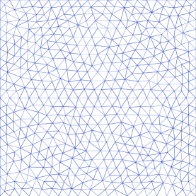
(a): meshIso, $N_{e}=964$

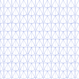
(b): meshAcute, $N_{e}=800$

(c): mesh45, $N_{e}=800$

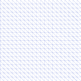
(d): mesh135, $N_{e}=800$

Figure 2: Different meshes used in the numerical computations.

The first example is an isotropic problem with a known exact solution. The second example is anisotropic but homogeneous, that is, the diffusion matrix is constant but has different eigenvalues. The last example is anisotropic and inhomogeneous where the diffusion matrix not only has different eigenvalues and but also varies in location. For simplicity, we only consider the cases when the diffusion matrix is time independent.

      Example 6.1.

The first example is in the form of (1) with $\Omega=(-100,100)\times(-100,100)$, $\mathbb{D}=I$, and $g(x,y,t)$ and $u_{0}(x,y)$ are given such that the equation (1) has the exact solution

$$u(x,y,t)=\frac{e^{0.5(x+y)+(0.5-0.1)t}}{e^{0.5(x+y)+(0.5-0.1)t}+2},$$ (68)

which satisfies $0\leq u\leq 1$.

We first verify the convergence order of the schemes. The $L^{2}$-norm of the error using the four methods (EM, IM, HEIM1, HEIM2) with mesh45 is scaled by the square root of the area of the domain. For the convergence in time, $T=10$ and a fixed, fine mesh with $N_{e}=2,000,000$ are used in the computations. The results are shown in Fig. 3, which clearly show first order convergence in time. It is interesting to point out that HEIM I has the smallest error while HEIM II has the largest one.

For the convergence in space, $T=0.25$ and $\Delta t=10^{-4}$ are used in the computations. A small time step is used so that the temporal discretization error stays at a negligible level. The results are shown in Fig. 4. They demonstrate a second order convergence in space (i.e., $\mathcal{O}(1/N_{e})$). One may notice that the error for the four approximations is indistinguishable since they have similar spatial discretization errors.

We remark that the schemes show a similar convergence behavior on other meshes. The results are not presented here to save space. Moreover, the diffusion for this example is isotropic and the ANOAC condition (that is, $D_{acute}\geq 0$) reduces to the conventional nonobtuse-angle condition. We have $D_{acute}=-0.277$ for meshIso shown in Fig. 2(a) (which has obtuse triangles), $D_{acute}=0$ for both mesh45 and mesh135, and $D_{acute}=0.0116$ for meshAcute. Thus, only meshAcute satisfies the mesh conditions in Theorems 3.1, 3.2, 3.3, and 3.4 which essentially require the mesh to be acute. Nevertheless, the numerical solutions obtained from all the four methods on all the meshes do not violate the solution nonnegativitiy when the mesh is sufficiently fine. This is because those are only sufficient conditions. The numerical solution is guaranteed to satisfy the nonnegativity when the conditions are met and there is no such guarantee otherwise. The next example will demonstrate this.

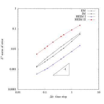
Figure 3: Example 6.1. The $L^{2}$-norm of the error for different time steps using mesh45 with $N_{e}=2,000,000$ and $T=10.0$.

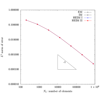
Figure 4: Example 6.1. The $L^{2}$-norm of the error for different mesh sizes using mesh45 with $\Delta t=1.0\times 10^{-4}$ and $T=0.25$.

      Example 6.2.

This example has the same boundary and initial conditions as Example 6.1 but its domain is $\Omega=(-100,100)\times(-170,170)$ and the diffusion matrix is anisotropic and homogeneous (i.e., not changing with location),

$$\mathbb{D}=\frac{1}{4}\left[\begin{array}[]{cc}203&199\sqrt{3}\\ 199\sqrt{3}&601\end{array}\right].$$ (69)

This anisotropic diffusion matrix has eigenvalues $\lambda_{1}=200$ and $\lambda_{2}=1$, and the eigenvector corresponding to the principal eigenvalue $\lambda_{1}$ is in the direction of $60$ degree. There is no exact solution available; however, the solution should lie in the interval $(0,1)$ according to the preservation of nonnegativity and boundedness.

Notice that the domain is no longer square. Indeed, the hypotenuse side of each triangle element in mesh45 is now in the direction of $59.5$ degree instead of $45$ degree as in the previous example. For convenience and without confusion, we still denote the mesh as mesh45. The situation is similar for mesh135. Table 1 shows the values of $D_{acute}$ and $D_{acute,ave}$ for the four meshes, where $D_{acute,ave}$ is an averaged indicator of $D_{acute}$ defined as

$$\mathbb{D}_{acute,ave}=\frac{1}{N}\sum\limits_{K\in\mathcal{T}_{h}}\left(\frac{|\Omega|}{N_{e}}\right)^{\frac{2}{d}}\min\limits_{\begin{subarray}{c}i,j=0,...,d\\ i\neq j\end{subarray}}(-(\nabla\phi_{i})^{T}\mathbb{D}_{K}\nabla\phi_{j}).$$ (70)

As can be seen from Table 1, the values of $\mathbb{D}_{acute}$ are negative for all meshes except mesh45. Thus, none of the meshIso, mesh135 and meshAcute satisfies the anisotropic acute angle condition. On the other hand, the elements of mesh45 are closely aligned along the principal diffusion direction and the positive $\mathbb{D}_{acute}$ implies that the mesh satisfies the anisotropic acute angle condition.

The numerical solutions at $T=40$ obtained with time step $\Delta t=0.1$ for the four meshes are shown in Fig. 5. Table 2 lists the minimum and maximum values in the numerical solutions, denoted by $u_{min}$ and $u_{max}$, respectively. The numerical solutions from all meshes except mesh45 has negative values (undershoot) and values larger than 1 (overshoot), which violate the nonnegativity and upper boundedness. The regions of undershoot and overshoot are displayed in Fig. 5 as empty white areas. Only the solutions obtained from mesh45 are guaranteed to stay within [0,1].

It is instructive to see that the upper bound of the time step is $\Delta t_{ub}=10$ in (30) for EM method, $\Delta t_{ub}=3.3$ in (39) for IM, $\Delta t_{ub}=4.9$ in (50) for HEIM I, and $\Delta t_{ub}=\infty$ in (57) for HEIM II (i.e., no upper bound). As mentioned in the previous sections, they are not really a restriction in practical computation.

The results using lumped mass and reaction terms are presented in Table 3. With lumping technique, the results are close to those without lumping (Table 2) but with slight improvements. For example, using HEIM II method, $u_{min}$ and $u_{max}$ are improved from $-0.0092$ and $1.0041$ without lumping to $-0.0088$ and $1.0035$ with lumping, respectively. Recall that the situations with lumping have less restrictive requirements on time step but the mesh condition is almost the same as for those without lumping.

Table 1: Measures for satisfaction of the anisotropic non-obtuse angle condition for Example 6.2.

Mesh	meshIso	mesh45	mesh135	meshAcute
$N_{e}$	51,190	51,200	51,200	51,200
$\mathbb{D}_{acute}$	-1.7e+2	5.3e-2	-4.3e+1	-2.0e+2
$\mathbb{D}_{acute,ave}$	-2.3e+1	5.3e-2	-4.3e+1	-5.8e+1

(a): meshIso, $N_{e}=51,190$

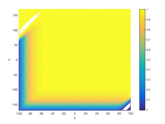
(b): meshAcute, $N_{e}=51,200$

(c): mesh45, $N_{e}=51,200$

(d): mesh135, $N_{e}=51,200$

Figure 5: Example 6.2. Filled contour plot of the numerical solutions at $T=40$ obtained from different meshes with $\Delta t=0.1$. The regions of undershoot and overshoot are displayed as empty white areas.

Table 2: Numerical solutions obtained using different meshes and methods for Example 6.2.

Mesh	solution	EM	IM	HEIM I	HEIM II
meshIso	$u_{min}$	-3.1e-3	-3.1e-3	-3.1e-3	-3.1e-3
$N_{e}=51,190$	$u_{max}$	1.0004	1.0003	1.0004	1.0003
mesh45	$u_{min}$	0	0	0	0
$N_{e}=51,200$	$u_{max}$	1	1	1	1
mesh135	$u_{min}$	-8.1e-3	-8.1e-3	-8.1e-3	-8.1e-3
$N_{e}=51,200$	$u_{max}$	1.0041	1.0040	1.0040	1.0040
meshAcute	$u_{min}$	-9.2e-3	-9.3e-3	-9.3e-3	-9.2e-3
$N_{e}=51,200$	$u_{max}$	1.0041	1.0040	1.0041	1.0040

Table 3: Numerical solutions obtained using different meshes and methods for Example 6.2 with lumped mass and reaction terms.

Mesh	solution	EM	IM	HEIM I	HEIM II
meshIso	$u_{min}$	-2.8e-3	-2.9e-3	-2.9e-3	-2.8e-3
$N_{e}=51,190$	$u_{max}$	1.0003	1.0002	1.0002	1.0002
mesh45	$u_{min}$	0	0	0	0
$N_{e}=51,200$	$u_{max}$	1	1	1	1
mesh135	$u_{min}$	-8.0e-3	-8.0e-3	-8.0e-3	-8.0e-3
$N_{e}=51,200$	$u_{max}$	1.0037	1.0037	1.0037	1.0037
meshAcute	$u_{min}$	-8.8e-3	-8.8e-3	-8.8e-3	-8.8e-3
$N_{e}=51,200$	$u_{max}$	1.0035	1.0034	1.0035	1.0034

      Example 6.3.

In this example, we consider a diffusion matrix that is anisotropic and inhomogeneous (i.e., location dependent). Specifically, we choose the diffusion matrix in the form

$$\mathbb{D}=\left[\begin{array}[]{ll}\cos\theta&-\sin\theta\\ \sin\theta&\cos\theta\end{array}\right]\left[\begin{array}[]{ll}200&0\\ 0&1\end{array}\right]\left[\begin{array}[]{ll}\cos\theta&\sin\theta\\ -\sin\theta&\cos\theta\end{array}\right],$$ (71)

where $\theta=\theta(x,y)$ is the angle of the tangential direction at point $(x,y)$ along concentric circles centered at (0,0). The domain and the boundary and initial conditions are chosen the same as in Example 6.1. The solution also preserves nonnegativity and boundedness and should stay within $[0,1]$.

For this example, none of meshIso, mesh45, mesh135, and meshAcute satisfies the corresponding mesh conditions, as can be seen from the values of $\mathbb{D}_{acute}$ in Table 4. For the purpose of comparison, another mesh, denoted by meshDMP, is generated according to the metric tensor $\mathbb{M}_{K}=\mathbb{D}_{K}^{-1}$ as proposed in [28]. The elements in meshDMP are made to be aligned along the principal diffusion direction as much as possible, as shown in Fig. 6. However, it is impossible to force every element in the square domain to be aligned along the concentric direction. Some elements that are not aligned well will violate the mesh condition and lead to negative $\mathbb{D}_{acute}$ value ($\mathbb{D}_{acute}=-1500$). On the other hand, $\mathbb{D}_{acute,ave}=1.1$, which indicates that most elements in the mesh satisfy the mesh condition. In this sense, meshDMP can be considered to closely satisfy the anisotropic acute angle condition for the given diffusion matrix.

Table 5 shows the minimum and maximum values of the numerical solutions obtained from the five meshes. Both undershoot and overshoot are observed in the solutions obtained with meshIso, mesh45, mesh135, and meshAcute whereas the solutions obtained from meshDMP stay within [0, 1]. The numerical solutions at $T=40$ obtained using different meshes and $\Delta t=0.1$ are shown in Fig. 7 where the regions of undershoot and overshoot are displayed as empty white areas. The numerical solution obtained from meshDMP with $N_{e}=51,146$ does not have undershoot and overshoot. When the mesh is being refined, undershoot and overshoot vanish from the numerical solution for meshIso with $N_{e}=591,506$ but are still present in the solutions obtained with much finer mesh45, mesh135, or meshAcute.

The results with lumped mass and reaction terms are shown in Table 6. Like Example 6.2, there are slight improvements by using lumping technique. One notable improvement is that $u_{min}$ for mesh135 is 0, that is, no undershoot is observed for results obtained using mesh135 with lumped mass and reaction terms.

Table 4: Measures for the satisfaction of the anisotropic non-obtuse angle condition for Example 6.3.

Mesh	meshIso	mesh45	mesh135	meshAcute	meshDMP
$N_{e}$	51,910	51,200	51,200	51,200	51,146
$\mathbb{D}_{acute}$	-1.2e+2	-5.0e+1	-5.0e+1	-2.6e+2	-1.5e+3
$\mathbb{D}_{acute,ave}$	-1.8e+1	-2.3e+1	-2.3e+1	-5.0e+1	1.1

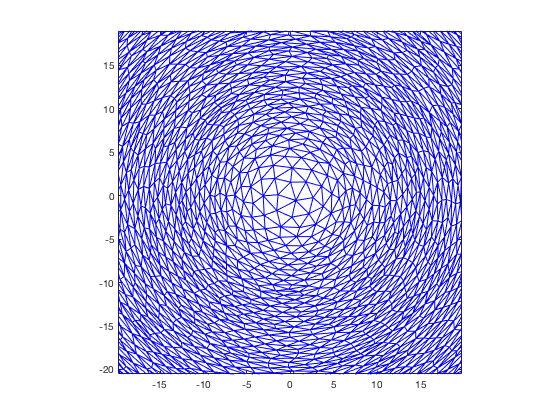
Figure 6: Example 6.3. Scaleup view of meshDMP at (0,0).

Table 5: Numerical solutions obtained from different meshes and methods for Example 6.3.

Mesh	solution	EM	IM	HEIM I	HEIM II
meshIso	$u_{min}$	-1.3e-3	-1.2e-3	-1.3e-3	-1.4e-3
$N_{e}=51,910$	$u_{max}$	1.0129	1.0129	1.0129	1.0129
mesh45	$u_{min}$	-1.4e-2	-1.4e-2	-1.4e-2	-1.5e-2
$N_{e}=51,200$	$u_{max}$	1.0101	1.0101	1.0101	1.0101
mesh135	$u_{min}$	-4.4e-6	-3.0e-6	-3.8e-6	-8.4e-6
$N_{e}=51,200$	$u_{max}$	1.0082	1.0082	1.0082	1.0082
meshAcute	$u_{min}$	-1.0e-2	-1.0e-2	-1.0e-2	-1.1e-2
$N_{e}=51,200$	$u_{max}$	1.0165	1.0165	1.0165	1.0164
meshDMP	$u_{min}$	0	0	0	0
$N=51,146$	$u_{max}$	1	1	1	1

(a): meshIso, $N_{e}=51,910$

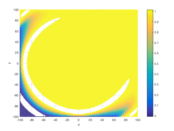
(b): meshAcute, $N_{e}=51,200$

(c): mesh45, $N_{e}=51,200$

(d): mesh135, $N_{e}=51,200$

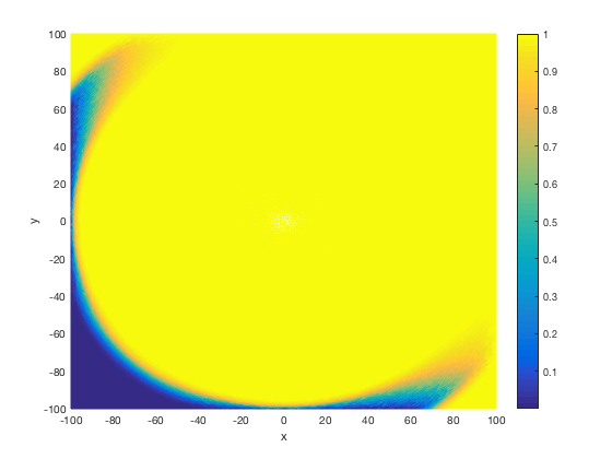
(e): meshDMP, $N_{e}=51,146$

Figure 7: Example 6.3. Filled contour plot of the numerical solutions at $T=40$ obtained from different meshes with $\Delta t=0.1$. The regions of undershoot and overshoot are displayed as empty white areas.

Table 6: Numerical solutions obtained from different meshes and methods for Example 6.3 with lumped mass and reaction terms.

Mesh	solution	EM	IM	HEIM I	HEIM II
meshIso	$u_{min}$	-1.2e-3	-1.2e-3	-1.2e-3	-1.2e-3
$N_{e}=51,910$	$u_{max}$	1.0111	1.0111	1.0111	1.0111
mesh45	$u_{min}$	-1.5e-2	-1.5e-2	-1.5e-2	-1.5e-2
$N_{e}=51,200$	$u_{max}$	1.0087	1.0087	1.0087	1.0087
mesh135	$u_{min}$	0	0	0	0
$N_{e}=51,200$	$u_{max}$	1.0068	1.0068	1.0068	1.0068
meshAcute	$u_{min}$	-1.0e-2	-1.0e-2	-1.0e-2	-1.1e-2
$N_{e}=51,200$	$u_{max}$	1.0115	1.0115	1.0115	1.0115
meshDMP	$u_{min}$	0	0	0	0
$N=51,146$	$u_{max}$	1	1	1	1

7 Conclusions

Nagumo-type equations arise from different fields and have been widely studied. However, preservation of the nonnegativity and boundedness in the numerical solution remains an important and challenge task. Some results have been obtained for the finite difference solution with isotropic diffusion, but little is known for the finite element solution especially with anisotropic diffusion.

In the previous sections we have studied the numerical solution of Nagumo-type equations with both isotropic and anisotropic diffusion. Linear finite elements on simplicial meshes and the backward Euler scheme have been used for the spatial and temporal discretization, respectively. Four different treatments for the nonlinear reaction term have been considered, including the explicit method (EM), the fully implicit method (IM), and two hybrid explicit-implicit methods (HEIM I and HEIM II). The conditions for the mesh and the time step have been developed for the numerical solution to preserve the nonnegativity and/or boundedness of the solution of the continuous problem. They are stated in Theorems 3.1, 3.2, 3.3, and 3.4. Roughly speaking, the mesh conditions require that the mesh be at least acute in the metric $\mathbb{D}^{-1}$ where $\mathbb{D}$ is the diffusion matrix while the time step conditions ask the time step to be bounded below and above. An only exception is HEIM II which does not have an upper bound placed on the time step. Moreover, if the mesh is uniformly acute in the metric $\mathbb{D}^{-1}$ as it is being refined, the time step conditions essentially become

$$\mathcal{O}(h^{2})\leq\Delta t_{n}\leq\mathcal{O}(1),$$

which can be satisfied easily when the mesh is sufficiently fine.

We have also studied the effects of lumping on the mass matrix and reaction term. The analysis shows that lumping not only removes the low bound requirement for the time step but also relaxes the requirement on the mesh for the numerical solution to preserve the nonnegativity and/or boundedness. Indeed, with lumping the conditions only require that the mesh be nonobtuse in the metric $\mathbb{D}^{-1}$ and the time step be bounded as

$$\Delta t_{n}\leq\mathcal{O}(1).$$

Once again, there is no upper bound for $\Delta t_{n}$ for HEIM II.

HEIM II leads to the weakest conditions among the four approximations for the reaction term. However, numerical experiment shows that other approximations give smaller temporal discretization errors. Numerical examples also confirm the first order convergence in time and second order convergence in space for the scheme with all four approximations to the reaction term.

Acknowledgments. The authors are grateful to Erik Van Vleck for his valuable comments in improving the quality of the paper.

References

- [1] S. Abbasbandy. Soliton solutions for the Fitzhugh-Nagumo equation with the homotopy analysis method. Appl. Math. Model., 32:2706–2714, 2008.
- [2] J.G. Alford and G. Auchmuty. Rotating wave solutions of the Fitzhugh-Nagumo equations. J. Math. Biol., 53:797–819, 2006.
- [3] U.M. Ascher, S.J. Ruuth, and R.J. Spiteri. Implicit-explicit Runge-Kutta methods for time-dependent partial differential equations. Appl. Numer. Math., 25:151–167, 1997.
- [4] U.M. Ascher, S.J. Ruuth, and B.T.R. Wetton. Implicit-explicit methods for time-dependent partial differential equations. SIAM J. Numer. Anal., 32:797–823, 1995.
- [5] J. Brandts, S. Korotov, and M. Křížek. Dissection of the path-simplex in into path-subsimplices. Lin. Alg. Appl., 421:382–393, 2007.
- [6] J. Brandts, S. Korotov, M. Křížek, and J. Šolc. On nonobtuse simplicial partitions. SIAM Rev., 51:317–335, 2009.
- [7] Z. Chen, A.B. Gumel, and R.E. Mickens. Nonstandard discretizations of the generalized nagumo reaction-diffusion equation. Numer. Meth. P.D.E., 19:363–379, 2003.
- [8] P.G. Ciarlet. The Finite Element Method for Elliptic Problems. North-Holland, Amsterdam, 1978.
- [9] P.G. Ciarlet and P.-A. Raviart. Maximum principle and uniform convergence for the finite element method. Comput. Methods Appl. Mech. Engrg., 2:17–31, 1973.
- [10] E.M. Constantinescu and A. Sandu. Extrapolated implicit-explicit time stepping. SIAM J.Sci. Comput., 31:4452–4477, 2010.
- [11] B. Deng. The existence of infinitely many traveling front and back waves in the Fitzhugh-Nagumo equations. SIAM J. Math. Anal., 22:1631–1650, 1991.
- [12] A. Dikansky. Fitzhugh-Nagumo equations in a nonhomogeneous medium. Dis. Con. Dyn. Sys., Supplement:216–224, 2005.
- [13] L. C. Evans. Partial Differential Equations. American Mathematical Society, Providence, RI, 1998.
- [14] I. Faragó and R. Horváth. Discrete maximum principle and adequate discretizations of linear parabolic problems. SIAM J. Sci. Comput., 28:2313–2336, 2006.
- [15] I. Faragó, R. Horváth, and S. Korotov. Discrete maximum principle for fe solutions of nonstationary diffusion-reaction problems with mixed boundary conditions. Numer. Meth. P.D.E., 27:702–720, 2011.
- [16] I. Faragó, J. Karátson, and S. Korotov. Discrete maximum principle for nonlinear parabolic PDE systems. IMA J. Numer. Anal., 32:1541–1573, 2012.
- [17] R. FitzHugh. Impulses and physiological states in theoretical models of nerve membrane. Biophysical J., 1:445–466, 1961.
- [18] S. Göktepe and E. Kuhl. Computational modeling of cardiac electrophysiology: A novel finite element approach. Int. J. Numer. Meth. Engrg., 79:156–178, 2009.
- [19] J. Guckenheimer and C. Kuehn. Homoclinic orbits of the Fitzhugh-Nagumo equation: Bifurcations in the full system. SIAM J. Appl. Dyn. Sys., 9:138–153, 2010.
- [20] S.P. Hastings. On the existence of homoclinic and periodic orbits in the Fitzhugh-Nagumo equations. Quart. J. Math. Oxford, 2:123–134, 1976.
- [21] F. Hecht. Bidimensional anisotropic mesh generator software (BAMG). http://www.ann.jussieu.fr/hecht/ftp/bamg/bamg-v1.01.tar.gz, 2010.
- [22] C. Jones. Stability of the traveling wave solution of the Fitzhugh-Nagumo system. Trans. Amer. Math. Soc., 286:431–469, 1984.
- [23] A. Kanevsky, M.H. Carpenter, D. Gottlieb, and J.S. Hesthaven. Application of implicit-explicit high order Runge-Kutta methods to discontinuous-Galerkin schemes. J. Comp. Phys., 225:1753–1781, 2007.
- [24] J. Keener and J. Sneyd. Mathematical Physiology. Springer-Verlag, New York, 1998.
- [25] T. Kostova, R. Ravindran, and M. Schonbek. Fitzhugh-Nagumo revisited: Types of bifurcations, periodical forcing and stability regions by a Lyapunov functional. Int. J. Bif. Chaos, 14:913–925, 2004.
- [26] M. Krupa, B. Sandstede, and P. Szmolyan. Fast and slow waves in the Fitzhugh-Nagumo equation. J. Diff. Eq., 133:49–97, 1997.
- [27] C. Lenk, M. Einax, and P. Maass. Wavefront-obstacle and wavefront-wavefront interactions as mechanisms for atrial fibrillation: A study based on the Fitzhugh-Nagumo equations. Comput. Cardiology, 37:425–428, 2010.
- [28] X. Li and W. Huang. An anisotropic mesh adaptation method for the finite element solution of heterogeneous anisotropic diffusion problems. J. Comput. Phys., 229:8072–8094, 2010.
- [29] X. Li and W. Huang. Maximum principle for the finite element solution of time-dependent anisotropic diffusion problems. Numer. Meth. P.D.E., 29:1963–1985, 2013.
- [30] W. Liu and E. Van Vleck. Turning points and traveling waves in Fitzhugh-Nagumo type equations. J. Diff. Eq., 225:381–410, 2006.
- [31] C. Lu, W. Huang, and J. Qiu. Maximum principle in linear finite element approximations of anisotropic diffusion-convection-reaction problems. Numer. Math., 127:515–537, 2014.
- [32] J.E. Macías-Díaz. On a boundedness-preserving semi-linear discretization of a two-dimensional non-linear diffusion-reaction model. Int. J. Comput. Math, 89:1678–1688, 2012.
- [33] M.E. Mazurov and I.M. Kalyuzhnyi. Circular autowaves in human atria and initial conditions for their emergence. Moscow University Physics Bulletin, 69:251–256, 2014.
- [34] H.P. McKean. Nagumo’s equation. Adv. Math., 4:209–223, 1970.
- [35] A.S. Mikhailov and K. Showalter. Control of waves, patterns and turbulence in chemical systems. Physics Reports, 425:79–194, 2006.
- [36] J. Nagumo, S. Arimoto, and S. Yoshizawa. An active pulse transmission line simulating a nerve axon. Proc. Institute of Radio Engineers, 50:2061–2070, 1962.
- [37] R.J. Plemmons. M-matrix characterizations. I. Nonsingular M-matrices. Lin. Alg. Appl., 18:175–188, 1977.
- [38] C. Le Potier. A nonlinear finite volume scheme satisfying maximum and minimum principles for diffusion operators. Int. J. Finite Vol., 6:20, 2009.
- [39] W. Qin, D. Ding, and X. Ding. Unconditionally positivity and boundedness preserving schemes for a Fitzhugh-Nagumo equation. Int. J. Comput. Math., 92:2198–2218, 2015.
- [40] I. Ratas and K. Pyragas. Effect of high-frequency stimulation on nerve pulse propagation in the Fitzhugh-Nagumo model. Nonlin. Dyn., 67:2899–2908, 2012.
- [41] J. Ruiz-Ramírez and J.E. Macías-Díaz. A finite-difference scheme to approximate non-negative and bounded solutions of a Fitzhugh-Nagumo equation. Int. J. Comput. Math., 88:3186–3201, 2011.
- [42] M.C. Tanzy, V.A. Volpert, A. Bayliss, and M.E. Nehrkorn. A Nagumo-type model for competing populations with nonlocal coupling. Math. Biosciences, 263:70–82, 2015.
- [43] J. Wang and R. Zhang. Maximum principle for P1-conforming finite element approximations of quasi-linear second order elliptic equations. SIAM J. Numer. Anal., 50:626–642, 2012.
- [44] J. Wong, S. Göktepe, and E. Kuhl. Computational modeling of electrochemical coupling: A novel finite element approach towards ionic models for cardiac electrophysiology. Comput. Methods Appl. Mech. Engrg., 200:3139–3158, 2011.
- [45] E. Yanagida. Stability of fast traveling pulse solutions of the Fitzhugh-Nagumo equation. J. Math. Biol., 22:81–104, 1985.
- [46] G. Yuan and Z. Sheng. Monotone finite volume schemes for diffusion equations on polygonal meshes. J. Comput. Phys., 227:6288–6312, 2008.
- [47] X. Zhang and C.W. Shu. Maximum-principle-satisfying and positivity-preserving high-order schemes for conservation laws: Survey and new developments. Proc. R. Soc. A Math. Phys. Eng. Sci., 467:2752–2776, 2011.