SLANTS: Sequential Adaptive Nonlinear Modeling of Vector Time Series

Abstract

We propose a method for adaptive nonlinear sequential modeling of vector-time series data. Data is modeled as a nonlinear function of past values corrupted by noise, and the underlying non-linear function is assumed to be approximately expandable in a spline basis. We cast the modeling of data as finding a good fit representation in the linear span of multi-dimensional spline basis, and use a variant of $l_{1}$-penalty regularization in order to reduce the dimensionality of representation. Using adaptive filtering techniques, we design our online algorithm to automatically tune the underlying parameters based on the minimization of the regularized sequential prediction error. We demonstrate the generality and flexibility of the proposed approach on both synthetic and real-world datasets. Moreover, we analytically investigate the performance of our algorithm by obtaining both bounds of the prediction errors, and consistency results for variable selection.

I Introduction

Sequentially observed vector-time series are emerging in various applications. In most these applications modeling nonlinear functional inter-dependency between present and past data is crucial for both representation and prediction. This is a challenging problem given that often in various applications fast online implementation, adaptivity and ability to handle high dimensions are basic requirements for nonlinear modeling. For example, environmental science combines high dimensional weather signals for real time prediction [1]. In epidemics, huge amount of online search data is used to form fast prediction of influenza epidemics [2]. In finance, algorithmic traders demand adaptive models to accommodate a fast changing stock market. In robot autonomy, there is the challenge of learning the high dimensional movement systems [3]. These tasks usually take high dimensional input signals which may contain a large number of irrelevant signals. In all these applications, clearly methods to remove redundant signals, and learn the nonlinear model with low computational complexity are well sought after. This motivates our work in this paper, where we propose an approach to sequential nonlinear adaptive modeling of potentially high dimensional vector time series.

Inference of nonlinear models has been a notoriously difficult problem, especially for large dimensional data[4, 3, 5]. In low dimensional settings, there have been remarkable parametric and nonparametric nonlinear time series models that have been applied successfully to data from various domains. Examples include threshold models[6], generalized autoregressive conditional hetero-scedasticity models[7], multivariate adaptive regression splines (MARS)[4], generalized additive models[8], functional coefficient regression models[9], etc. However, some of these methods may suffer from prohibitive computational complexity. Model selection using some of these approaches is yet another challenge as they may not eliminate insignificant predictors. In contrast, there exist high dimensional nonlinear time series models (3) that are mostly inspired by high dimensional statistical methods. In one approach, a small subset of significant variables is first selected and then nonlinear time series models are applied to selected variables. For example, independence screening techniques such as [10, 11, 12] or the MARS may be used to do variable selection. In another approach, dimension reduction method such as least absolute shrinkage and selection operator (LASSO) [13] are directly applied to nonlinear modeling. Sparse additive models have been developed in recent works of Ravikumar [14] and Huang[5]. These approaches seem to be very promising, and may benefit from additional reductions in computational complexity.

In this work, we will build on the latter category and develop an adaptive and online model for nonlinear modeling. Our method is sequential which provides computational benefits as we avoid applying batch estimation up on sequential arrival of data. It also provides resilience to time-variation of data, which may be important as in many practical applications [1, 2, 3], the functional dependency between present and past data seems to be time-varying. In fact, it is widely believed that a robust inference procedure must be adaptive to new environments (data generating processes). However, it is common to assume that these time-variations are smooth [15], and this assumption will be made in the sequel. Using this smoothness assumption, we present a Sequential Learning Algorithm for Nonlinear Time Series (SLANTS). Specifically, we will use the spline basis to dynamically approximate the nonlinear functions. As common in adaptive filtering, we give a larger weights to more recent data points. We use group LASSO for dimensionality reduction in our simultaneous estimation and model selection, and for sequential update. To this end, we re-formulate our group LASSO regularization into a recursive estimation problem that produces an estimator close to the maximum likelihood estimator from batch data.

The outline of this paper is given next. In Section II, we formulate the problem mathematically and present our inference algorithm. In Section III, we present our theoretical results regarding prediction error and model consistency. In Section IV, we provide numerical results using both synthetic data and two sets of real data examples. The results demonstrate excellent performance of our methods.

II Sequential modeling of nonlinear time series

In this section, we first present our mathematical model and cast our problem as $l_{1}$-regularized linear regression . We then propose an EM type algorithm to sequentially estimate the underlying coefficients. Finally we disclose methods for tuning the underlying parameters. Combining our proposed EM estimation method with automatic parameter tuning, we tailor our algorithm to sequential vector time series applications.

II-A Formulation of SLANTS

Consider a multi-dimensional vector time series given by

$$\bm{X}_{t}=[X_{1,t},\ldots,X_{D,t}]^{\mathrm{\scriptscriptstyle T}}\in\mathbb{R}^{D},t=1,2,\ldots$$

Our main objective in this paper is to predict the value of $\bm{X}_{T}$ at time $T$ given the past observations $\bm{X}_{T-1},\ldots,\bm{X}_{1}$. Without loss of generality, for simplicity we present our results for the prediction of scalar random variable $X_{1,T+1}$. Let $\bm{X}_{t,-j}=[X_{1,t},\ldots,X_{j-1,t},X_{j+1,t},\ldots,X_{D,t}]^{\mathrm{\scriptscriptstyle T}}.$ We start with a general formulation

$$X_{1,T}=f(\bm{X}_{T,-1},\bm{X}_{T-1},\ldots,\bm{X}_{T-L})+{\varepsilon}_{T}$$ (1)

where $f(\cdot,\cdots,\cdot)$ is smooth (or at least piece-wise smooth), ${\varepsilon}_{t}$ are independent and identically distributed (i.i.d.) zero mean random variables and the lag order $L$ is a finite but unknown nonnegative integer.

This general formulation encompasses three special but important cases. The first case is when $L=0$, and there is only instantaneous functional relationship among random variables: $X_{1,T}=f(\bm{X}_{T,-1})+{\varepsilon}_{T}$ and this is just a standard regression problem. The second case is when $D=1$, and the Equation (1) reduces to the one-dimensional (non)linear autoregressive model. The third case is when $f(\cdot,\cdots,\cdot)$ includes variables related to only times before $t$.

$$X_{1,T}=f(\bm{X}_{T-1},\ldots,\bm{X}_{T-L})+{\varepsilon}_{T}.$$ (2)

This case is of practical interest for prediction purposes. We rewrite the model in (2) as

$$X_{1,T} =f(X_{1,T-1},\ldots,X_{1,T-L},\ldots,X_{D,T-1},\ldots,X_{D,T-L})+{\varepsilon}_{T}.$$

With a slight abuse of notation, we rewrite the above model as

$$Y_{T}=f(X_{1,T},\ldots,X_{\tilde{D},T})+{\varepsilon}_{T}$$ (3)

with observations $Y_{T}=X_{1,T}$ and $[X_{1,T},\ldots,X_{\tilde{D},T}]$ $=$ $[X_{1,T-1},\ldots,X_{1,T-L},\ldots,X_{D,T-1},\ldots,X_{D,T-L}]$, where $\tilde{D}=DL$. To estimate $f(\cdot,\cdots,\cdot)$, we consider the following least squares formulation

$$\min_{f}\sum_{t=1}^{T}w_{T,t}(Y_{t}-f(X_{1,t},\ldots,X_{\tilde{D},t}))^{2}$$ (4)

where $\{w_{T,t}\in[0,1]\}$ are weights used to emphasize varying influences of the past data. The appropriate choice of $\{w_{T,t}\in[0,1]\}$ will be later discussed in section II-C.

In order to estimate the nonlinear function $f(\cdot,\cdots,\cdot)$ , we further assume a nonlinear additive model, i.e.

$$f(X_{1,t},\ldots,X_{\tilde{D},t})=\mu+\sum_{i=1}^{\tilde{D}}f_{i}(X_{i}),\quad E\{f_{i}(X_{i})\}=0,$$ (5)

where $f_{i}$ are scalar functions, and expectation is with respect to the stationary distribution of $X_{i}$. The second condition is required for identifiability. To estimate $f_{i}$, we use B-splines (extensions of polynomial regression techniques [16]). In our presentation, for brevity, we consider the additive model mainly but note that our methods can be extended to models where there exist interactions among $\bm{X}_{1},\ldots,\bm{X}_{\tilde{D}}$ using multidimensional splines in a straight-forward manner.

Incorporating the B-spline basis into regression, we write

$$f_{i}(x)=\sum_{j=1}^{v}c_{i,j}b_{i,j}(x),\quad b_{i,j}(x)=B(x\mid t_{i,1},\ldots,t_{i,v}),$$ (6)

where $t_{i,1},\ldots,t_{i,v}$ are the knot sequence and $b_{i,j}$ are the coefficients associated with the B-spline basis. Here, we have assumed that there are $v$ spline basis of degree $k$ for each $f_{i}$. Replacing these into (4), the problem of interest is now the minimization of

$$\hat{e}_{T}=\sum_{t=1}^{T}w_{T,t}\biggl{\{}Y_{t}-\mu-\sum_{i=1}^{\tilde{D}}\sum_{j=1}^{v}c_{i,j}b_{i,j}(X_{i,t})\biggr{\}}^{2}$$ (7)

over $c_{i,j},\,i=1,\ldots,\tilde{D},\,j=1,\ldots,v$, under the constraint

$$\sum_{t=1}^{T}\sum_{j=1}^{v}c_{i,j}b_{i,j}(x_{i})=0,\mbox{ for }i=1,\ldots,L$$ (8)

which is the sample analog of the constraint in (5). Equivalently, we obtain an unconstrained optimization problem by centering the basis functions. Let $b_{i,j}(x_{i,t})$ be replaced by $b_{i,j}(x_{i,t})-\frac{1}{T}\sum_{t=1}^{T}b_{i,j}(x_{i,t})$. By proper rearrangement, (7) can be rewritten into a linear regression form

$$\hat{e}_{T}=\sum_{t=1}^{T}w_{T,t}(Y_{T}-\bm{Z}_{T}\bm{\beta}_{T})^{2}$$ (9)

where $\bm{\beta}_{T}$ is a $(1+\tilde{D}v)\times 1$ column vector to be estimated and $\bm{Z}_{T}$ is $1\times(1+\tilde{D}v)$ row vector $\bm{Z}_{T}=[1,b_{1,1}(x_{1,T}),\ldots,b_{1,v}(x_{1,T}),\ldots,b_{\tilde{D},1}(x_{\tilde{D},T}),\ldots,b_{\tilde{D},v}(x_{\tilde{D},T})]$. Let $Z_{T}$ be the design matrix of stacking the row vectors $\bm{Z}_{t},t=1,\ldots,T$. Note that we have used $\bm{\beta}_{T}$ instead of a fixed $\bm{\beta}$ to emphasize that $\bm{\beta}_{T}$ may vary with time. We have used bold style for vectors to distinguish them from matrices. Let $W_{T}$ be the diagonal matrix whose elements are $w_{T,t},t=1,\ldots,T$. Then the optimal $\beta_{T}$ in (9) can be recognized as the MLE of the following linear Gaussian model

$$\bm{Y}_{T}=Z_{T}\bm{\beta}_{T}+\bm{{\varepsilon}}$$ (10)

where $\bm{{\varepsilon}}\in\mathcal{N}(0,W_{T}^{-1})$. Here, we have used $\mathcal{N}(\mu,\sigma^{2})$ to denote Gaussian distribution with mean $\mu$ and variance $\sigma^{2}$.

To obtain a sharp model from large $L$, we further assume that the expansion of $f(\cdot,\cdots,\cdot)$ is sparse, i.e., only a few additive components $f_{i}$ are active. Clearly, selecting a sparse model is critical as models of large dimensions lead to inflated variance whereas models of small dimension lead to the lack-of-fit bias. To this end, we give independent Laplace priors for each sub-vector of $\bm{\beta}_{T}$ corresponding to each $f_{i}$. Our objective now reduces to obtaining the maximum a posteriori estimator (MAP)

$$\log p(\bm{Y}_{T}\mid\bm{\beta}_{T})-\lambda_{T}\sum\limits_{i=1}^{\tilde{D}}\lVert\bm{\beta}_{T,i}\rVert_{2}.$$ (11)

The above prior corresponds to the so called group LASSO. The bold $\bm{\beta}_{T,i}$ is to emphasize that it is not a scalar element of $\bm{\beta}_{T}$ but a sub-vector of it. It will be interesting to consider adaptive group LASSO [17], i.e., to use $\lambda_{T,i}$ instead of a unified $\lambda_{T}$ and this is currently being investigated. We refer to [5] for a study of adaptive group LASSO for batch estimation.

II-B Implementation of SLANTS

In order to solve the optimization problem given by (11), we build on an EM-based solution originally proposed for wavelet image restoration [18]. This was further applied to online adaptive filtering for sparse linear models [15] and nonlinear models approximated by Volterra series [19, 20]. The basic idea is to decompose the optimization (11) into two parts that are easier to solve and iterate between them. One part involves linear updates, and the other involves group LASSO in the form of orthogonal covariance which leads to closed-form solution.

For now, we assume that the knot sequence $t_{i,1},\ldots,t_{i,v}$ for each $i$ and $v$ is fixed. Suppose that all the tuning parameters are well-defined. We introduce an auxiliary variable $\tau_{T}$ that we refer to as the innovation parameter. This helps us to decompose the problem so that underlying coefficients can be iteratively updated. It also allows the sufficient statistics to be rapidly updated in a sequential manner. The model in (10) now can be rewritten as

$$\bm{Y}_{T}=Z_{T}\bm{\theta}_{T}+W^{-\frac{1}{2}}\bm{{\varepsilon}}_{1},\ \bm{\theta}_{T}=\bm{\beta}_{T}+\tau_{T}\bm{{\varepsilon}}_{2},$$

where

$$\bm{{\varepsilon}}_{1}\in\mathcal{N}(0,I-\tau_{T}^{2}W^{\frac{1}{2}}Z_{T}Z_{T}^{\mathrm{\scriptscriptstyle T}}W^{\frac{1}{2}}),\quad\bm{{\varepsilon}}_{2}\in\mathcal{N}(0,I)$$ (12)

We treat $\bm{\theta}_{T}$ as the missing data, so that an EM algorithm can be derived. By basic calculations similar to that of [18], we obtain the $k$th step of EM algorithm

E step:

$$Q(\bm{\beta}\mid\hat{\bm{\beta}}^{(k)}_{T})=-\frac{1}{2\tau_{T}^{2}}\lVert\bm{\beta}-\bm{r}^{(k)}\rVert_{2}^{2}-\lambda_{T}\sum\limits_{i=1}^{\tilde{D}}\lVert\bm{\beta}_{i}\rVert_{2},$$ (13)

where

$$\bm{r}^{(k)}=(I-\tau^{2}A_{T})\hat{\bm{\beta}}^{(k)}_{T}+\tau^{2}B_{T},$$ (14)

$$A_{T}=Z_{T}^{\mathrm{\scriptscriptstyle T}}W_{T}Z_{T},\ \bm{B}_{T}=Z_{T}^{\mathrm{\scriptscriptstyle T}}W_{T}\bm{Y}_{T}.$$ (15)

M step: $\hat{\bm{\beta}}^{(k+1)}_{T}$ is the maximum of $Q(\bm{\beta}\mid\hat{\bm{\beta}}^{(k)}_{T})$ given by

$$\hat{\bm{\beta}}^{(k+1)}_{T,i}=\biggl{[}1-\frac{\lambda_{T}\tau_{T}^{2}}{\lVert\bm{r}^{(k)}_{i}\rVert_{2}}\biggr{]}_{+}\bm{r}^{(k)}_{i},\quad i=1,\ldots,\tilde{D}.$$ (16)

Suppose that we have obtained the estimator $\hat{\bm{\beta}}_{T}$ at time step $T$. Consider the arrival of the $(T+1)$th point $(y_{T+1},\bm{x}_{T+1})$, respectively corresponding to the response and covariates (as a row vector) of time step $T+1$. We first compute $\bm{r}^{(0)}_{T+1}$, the initial value of $\bm{r}$ to be input the EM at time step $T+1$:

$$\bm{r}^{(0)}_{T+1}=(I-\tau^{2}A_{T+1})\hat{\bm{\beta}}_{T}+\tau^{2}\bm{B}_{T+1},$$

where

$$A_{T+1} =(1-\gamma_{T+1})A_{T}+\gamma_{T+1}\bm{x}_{T+1}^{\mathrm{\scriptscriptstyle T}}\bm{x}_{T+1},$$

$$\bm{B}_{T+1} =(1-\gamma_{T+1})\bm{B}_{T}+\gamma_{T+1}y_{T+1}\bm{x}_{T+1}^{\mathrm{\scriptscriptstyle T}}.$$

Then we run the above EM for $K>0$ iterations to obtain an updated $\hat{\bm{\beta}}_{T+1}$.

In the following Theorem, we show EM converges exponentially fast to the MAP of (11). The proof is given in the appendix.

Theorem 1

At each iteration, the mapping from $\hat{\bm{\beta}}_{T}^{(k)}$ to $\hat{\bm{\beta}}_{T}^{(k+1)}$ is a contraction mapping for any $\tau_{T}$, whenever the absolute values of all eigenvalues of $I-\tau^{2}A_{T+1}$ are less than one. In addition, the error $\lVert\hat{\bm{\beta}}_{T}^{(k+1)}-\hat{\bm{\beta}}_{T}\rVert_{2}$ decays exponentially in $k$, where $\hat{\bm{\beta}}_{T}$ denotes the global minimum point of (11).

SLANTS can be efficiently implemented. In fact, by straightforward computations, the complexity of SLANTS at each time $t$ is $\Theta(\tilde{D}^{2})$. Coordinate descent [21] is perhaps the most widely used algorithm for batch LASSO. Adapting coordinate descent to sequential setting has the same complexity for updating sufficient statistics. However, it does not have any convergence rate guarantees that we know of. In contrast, SLANTS convergence is guaranteed by the above theorem.

II-C The choice of tuning parameters: from a prequential perspective

To evaluate the predictive power of an inferential model estimated from all the currently available data, ideally we would apply it to independent and identically generated datasets. However, it is not realistic to apply this cross-validation idea to real-world time series data, since real data is not permutable and has a “once in a lifetime” nature. As an alternative, we adopt a prequential perspective [22] that the goodness of a sequential predictive model shall be assessed by its forecasting ability.

Specifically, we evaluate the model in terms of the one-step prediction errors upon each newly arrived data point and subsequently tune the necessary control parameters, including regularization parameter $\lambda_{t}$ and innovation parameter $\tau_{t}$ (see details below). Automatic tuning of the control parameters are almost a necessity in many real-world applications in which any theoretical guidance (e.g., our Theorem 2) may be insufficient or unrealistic. Throughout our algorithmic design, we have adhered to the prequential principle and implemented the following strategies.

The choice of $w_{T,t}$: $w_{T,t}$ is determined by

$$w_{1,1} =\gamma_{1},\quad w_{t,j}=w_{t-1,j}(1-\gamma_{t}),\quad w_{t,t}=\gamma_{t},\,j=1,\ldots,t-1,$$

and $\{\gamma_{t}\}$ is a nonnegative sequence which we refer to as the step sizes. It includes two special cases that have been commonly used in the literature. The first case is $\gamma_{t}=1/t$. It is easy to verify that $w_{T,t}=1/T,t=1,\ldots,T$ for any $T$. This leads to the usual least squares. The second case is $\gamma_{t}=c$ where $c$ is a positive constant. It gives $w_{T,t}=c(1-c)^{T-t},t=1,\ldots,T$. From (4), the estimator of $f$ remains unchanged by rescaling $w_{T,t}$ by $1/c$, i.e. $w_{T,t}=(1-c)^{T-t}$ which is a series of powers of $1-c$. The value $1-c$ has been called the “forgetting factor” in the signal processing literature and used to achieve adaptive filtering [15].

The choice of $\tau_{T}$: Because the optimization problem

$$\log p(\bm{Y}_{T}\mid\bm{\beta}_{T})-\lambda_{T}\sum\limits_{i=1}^{L}\lVert\bm{\beta}_{T,i}\rVert_{2}$$ (17)

is convex, as long as $\tau_{T}$ is proper, the EM algorithm converges to the global optimum regardless of what $\tau_{T}$ is. But $\tau_{T}$ affects the speed of convergence of EM as $\lambda_{T}\tau_{T}^{2}$ determines how fast $\beta_{T}$ shrinks. Intuitively the larger $\tau_{T}$ is, the faster is the convergence. Therefore we prefer $\tau_{T}$ to be large and proper. A necessary condition for $\tau_{T}$ to be proper is to ensure that the covariance matrix of $\bm{{\varepsilon}}_{1}$ in

$$\bm{{\varepsilon}}_{1}\in\mathcal{N}(0,I-\tau_{T}^{2}W^{\frac{1}{2}}Z_{T}Z_{T}^{\mathrm{\scriptscriptstyle T}}W^{\frac{1}{2}}),\quad\bm{{\varepsilon}}_{2}\in\mathcal{N}(0,I)$$ (18)

is positive definite. Therefore, there is an upper bound $\bar{\tau}_{T}$ for $\tau_{T}$, and $\bar{\tau}_{T}$ converges to a positive constant $\bar{\tau}$ under some mild assumptions (e.g. the stochastic process $X_{t}$ is stationary). Extensive experiments have shown that $\bar{\tau}_{T}/2$ produces satisfying results in terms of model fitting. However, it is not computationally efficient to calculate $\bar{\tau}_{T}$ at each $T$ in SLANTS. Nevertheless without computing $\bar{\tau}_{T}$, we can determine if $\tau_{T}<\bar{\tau}_{T}$ by checking the EM convergence. If $\tau_{T}$ exceeds $\bar{\tau}_{T}$, the EM would diverge and coefficients go to infinity exponentially fast. This can be proved via a similar argument to that of proof of Theorem 1. This motivates a lazy update of $\tau_{T}$ with shrinkage only if EM starts to diverge.

The choice of $\lambda_{T}$: On the choice of regularization parameter $\lambda_{T}$, different methods have been proposed in the literature. The common way is to estimate the batch data for a range of different $\lambda_{T}$’s, and select the one with minimum cross-validation error. To reduce the underlying massive computation required for such an approach, in the context of Bayesian LASSO [23], [24] proposed an sequential Monte Carlo (SMC) based strategy to efficiently implement cross-validation. The main proposal is to treat the posterior distributions educed by an ordered sequence of $\lambda_{T}$ as $\pi_{t},t=0,1,\ldots$, the target distributions in SMC, and thus avoid the massive computation of applying Markov chain Monte Carlo (MCMC) for each $\lambda$ independently. Another method is to estimate the hyper-parameter $\lambda_{T}$ via empirical Bayes method [23]. In our context, however, it is not clear whether the Bayesian setting with MCMC strategy can be efficient, as the dimension $Lv$ can be very large. A possible implementation technique is to run three channels of our sequential modeling, corresponding to $\lambda_{T}^{-}=\lambda_{T}/\delta,\lambda_{T},\lambda_{T}^{+}=\lambda_{T}*\delta$, where $\delta>1$ is a small step size. The one with minimum average prediction error over the latest window of data was chosen as the new $\lambda_{T}$. For example, if $\lambda_{T}^{-}$ gives better performance, let the three channels be $\lambda_{T}^{-}/\delta,\lambda_{T}^{-},\lambda_{T}^{-}*\delta$. We also have a parameter $\nu$ that favors bigger $\lambda$ when comparing prediction error because we have measurement uncertainty of prediction error. That is, the prediction error is multiplied by $(\nu^{2},\nu,1)$ in 3 channels. $\nu$ affects the model performance in our experiments, especially the model sparsity. We now specify $\nu$ heuristically. It is ongoing work to fully understand how to specify $\nu$. If there is an underlying optimal $\lambda^{\ast}$ which does not depend on $T$, we would like our channels to converge to the optimal $\lambda^{\ast}$ by gradually shrinking the stepsize $\delta$. Specifically in case that the forgetting factor $\gamma_{t}=1/t$, we let $\delta_{T}=1+\frac{1}{T}(\delta-1)$ so that the step size $\delta_{T}\rightarrow 1$ at the same speed as weight of new data.

The choice of knots: The main difficulty in applying spline approximation is in determining the number of the knots to use and where they should be placed. Jupp [25] has shown that the data can be fit better with splines if the knots are free variables. de Boor suggests the spacing between knots is decreased in proportion to the curvature (second derivative) of the data. It has been shown that for a wide class of stationary process, the number of knots should be of the order of $O(T^{\zeta})$ for available sample size $T$ and some positive constant $\zeta$ to achieve a satisfying rate of convergence of the estimated nonlinear function to the underlying truth (if it exists) [26]. Nevertheless, under some assumptions, we will show in Theorem 2 that the prediction error can be upper bounded by an arbitrarily small number (which depends on the specified number of knots). It is therefore possible to identify the correct nonzero additive components in the sequential setting. On the other hand, using a fixed number of knots is computationally desirable because sharp selection of significant spline basis/support in a potentially varying environment is computationally intensive. It has been observed in our synthetic data experiments that the variable selection results are not very sensitive to the number of knots as long as this number is moderately large.

III Theoretical results

Consider the harmonic step size $\gamma_{t}=1/t$. For now assume that the sequential update at each time $t$ produces $\hat{\bm{\beta}}_{t}$ that is the same as the penalized least squares estimator given batch data. We are interested in two questions. First, how to extend the current algorithm in order to take into account an ever-increasing number of dimensions? Second, is it possible to select the “correct” nonzero components as sample size increases?

The first question is important in practice as any prescribed finite number of dimensions/time series may not contain the data-generating process, and it is natural to consider more candidates whenever more samples are obtained. It is directly related to the widely studied high-dimensional regression for batch data. In the second question, we are not only interested in optimizing the prediction error but also to obtain a consistent selection of the true nonzero components. Moreover, in order to maintain low complexity of the algorithm, we aim to achieve the above goal by using a fixed number of spline basis. We thus consider the following setup. Recall the predictive Model (2) and its alternative form (3). We assume that $L$ is fixed while $D$ is increasing with sample size $T$ at certain rate.

Following the setup of [27], we suppose that each $X_{d}$ takes values from a compact interval $[a,b]$. Let $[a,b]$ be partitioned into $J$ equal-sized intervals $\{I_{j}\}_{j=1}^{J}$, and let $\mathfrak{F}$ denote the space of polynomial splines of degree $\ell\geq 1$ consisting of functions $g(\cdot)$ satisfying 1) the restriction of $g(\cdot)$ to each interval is a polynomial of degree $\ell$, and 2) $g(\cdot)\in C^{\ell-1}[a,b]$ ($\ell-1$ times continuously differentiable). Typically, splines are called linear, quadratic or cubic splines accordingly as $\ell=1,2$, or $3$. There exists a normalized B-spline basis $\{b_{j}\}_{j=1}^{v}$ for $\mathfrak{F}$, where $v=J+\ell$, and any $f_{i}(x)\in\mathfrak{F}$ can be written in the form of (6). Let $k$ be a nonnegative integer, $\beta\in(0,1]$ that $p=k+\beta>0.5$, and $M>0$. Suppose each considered (non)linear function $f$ has $k$th derivative, $f^{(k)}$, and satisfies the Holder condition with exponent $\beta$: $|f^{(k)}(x)-f^{(k)}(x^{\prime})|<M|x-x^{\prime}|^{\beta}$ for $x,x^{\prime}\in[a,b]$. Define the norm $\lVert f\rVert_{2}=\sqrt{\int_{a}^{b}f(x)^{2}dx}$. Let $f^{*}\in\mathfrak{F}$ be the best $L_{2}$ spline approximation of $f$. Standard results on splines imply that $\lVert f_{d}-f^{*}_{d}\rVert_{\infty}=O(v^{-p})$ for each $d$. The spline approximation is usually an estimation under a mis-specified model class (unless the data-generating function is low-degree polynomials), and large $v$ narrows the distance to the true model. We will show that for large enough $v$, it is possible to achieve the aforementioned two goals. To make the problem concrete, we need the following assumptions on the data-generating procedure.

Assumption 1

The number of additive components is finite and will be included into the candidate set in finite time steps. In other words, there exists a “significant” variable set $S_{0}=\{i_{1},\ldots,i_{D_{0}}\}$ such that 1) $f_{d}(x)\neq 0$ for each $d\in S_{0}$, 2) $f_{d}(x)\equiv 0$ for $d\notin S_{0}$, and 3) both $D_{0}$ and $i_{D_{0}}$ are finite integers that do not depend on sample size $T$.

We propose two steps for a practitioner targeting two goals given below.

Step 1. (unbiasedness) This step aims to discover the significant variable set with probability close to one as more data is collected. The approach is to minimize the objective function in (11), and it can be efficiently implemented using the proposed sequential algorithm in Section II-B with negligible error (Theorem 1). In the case of equal weights $w_{T,t}=1/T$, it can be rewritten as

$$\lVert Y_{T}-Z_{T}\bm{\beta}_{T}\rVert_{2}^{2}+\tilde{\lambda}_{T}\sum\limits_{i=1}^{\tilde{D}}\lVert\bm{\beta}_{T,i}\rVert_{2}$$ (19)

where $\tilde{\lambda}_{T}=2T\lambda_{T}$. Due to Assumption 1, the significant variable set $S_{0}$ is included in the candidate set $\{1,\ldots,\tilde{D}\}$ for sufficiently large $T$. Our selected variables are those whose group coefficients are nonzero, i.e. $S_{1}=\{d:1\leq d\leq\tilde{D},\hat{\bm{\beta}}_{T,d}\neq\bm{0}\}$. We are going to prove that all the significant variables will be selected by minimizing (19) with appropriately chosen $\tilde{\lambda}_{T}$, i.e., $S_{0}\subseteq S_{1}$.

Step 2. (minimal variance) The second step is optional and it is applied only when a practitioner’s goal is to avoid selecting any redundant variables outside $S_{0}$. To achieve consistency of variable selection, we use the variables with nonzero estimated coefficients from Step 1 as candidate variables. Then we apply a BIC-type penalized method on future data points to further remove redundant variables. Suppose that we obtain a candidate set $S_{1}$ of $\tilde{D}$ variables (where $S_{0}\subseteq S_{1}$ from the Step 1) from fitting the sequential data upto $T_{1}=T/2$ and we perform the further procedure on data from $(T_{1}+1)$ to $T$. Since a thorough search over all subsets of variables is computationally demanding, we use a backward stepwise procedure. We start with the set of $S_{1}$ selected variables, delete one variable at a time by minimizing the MSE of a spline model with $v_{T}=T_{1}^{\zeta}$ number of equally spaced knots. Specifically, suppose that at step $k$ ($k=1,2,\ldots$), the survived candidate models are indexed by $\mathcal{S}^{(k)}$, we solve the least-squares problem for each $\bar{d}\in\mathcal{S}^{(k)}$

$$\hat{e}^{(k)}_{\bar{d}}=\min_{\mu,c_{d,j}}\sum_{t=T_{1}+1}^{T}\biggl{(}Y_{t}-\mu-\sum_{d\in\mathfrak{S}}\sum_{j=1}^{v_{T}}c_{d,j}b_{d,j}(X_{d,t})\biggr{)}^{2},$$ (20)

where $\mathfrak{S}=\mathcal{S}^{(k-1)}-\{\bar{d}\}$ and select $\bar{d}=\bar{d}_{k}^{*}$ that minimize the $\hat{e}^{(k)}_{\bar{d}}$ with minimum denoted by $\hat{e}^{(k)}$. Let $\mathcal{S}^{(k)}=\mathcal{S}^{(k-1)}-\bar{d}_{k}^{*}$. By default, we let $\mathcal{S}^{(0)}=S_{1}$ and use $\hat{e}^{(0)}$ to denote the minimum of (20) with $\mathfrak{S}=S_{1}$. If $\hat{e}^{(k-1)}-\hat{e}^{(k)}<(v_{T}\log T_{1})/T_{1}$ (the gain of goodness of fit is less than the incremented BIC penalty), then we stop the procedure and output $S_{2}=\mathcal{S}^{(k-1)}$; otherwise we proceed to the $(k+1)$th iteration. We prove that the finally selected subset $S_{2}$ satisfies $\lim_{T\rightarrow\infty}{\mathrm{pr}}(S_{2}=S_{0})=1$.

Before we proceed to the theoretical result, we introduce some necessary assumptions and their interpretations.

Assumption 2

There is a positive constant $c_{0}$ such that $\min_{d\in S_{0}}\lVert f_{d}\rVert_{2}\geq c_{0}$.

Assumption 3

The noises ${\varepsilon}_{t}$ are sub-Gaussian distributed, i.e., $E(e^{w{\varepsilon}_{t}})\leq e^{w^{2}\sigma^{2}/2}$ for a constant $\sigma>0$ and any $w\in\mathbb{R}$.

Assumption 4

Suppose that $S_{1}$ is a finite subset of $\{1,\ldots,\tilde{D}\}$. In addition, the “design matrix” $Z_{S_{1}}$ satisfies $Z_{S_{1}}^{\mathrm{\scriptscriptstyle T}}Z_{S_{1}}/T\geq\kappa$ for a positive constant $\kappa$ that depend only on $v$ (the number of splines).

We use $o_{p}(1)$ and $O_{p}(1)$ to denote a sequence of random variables that converges in probability to zero, and that is stochastically bounded, respectively. We use $O(1)$ to denote a bounded deterministic sequence.

Theorem 2

Suppose that Assumptions 1-4 hold. Then for any given $v$ it holds that

$$\lVert\bm{\beta}_{\tilde{S}_{1}}-\hat{\bm{\beta}}_{\tilde{S}_{1}}\rVert_{2}^{2}\leq 8c_{2}v^{-2p}/\kappa+O_{p}(T^{-1}\log\tilde{D})+O_{p}(T^{-1})+O(T^{-2}\tilde{\lambda}^{2})$$ (21)

for some positive constant $c_{2}$. If we further assume that $\log\tilde{D}=o(T)$, $\tilde{\lambda}=o(T)$, then there exists a constant $c_{1}>0$ such that for all $v>c_{1}c_{0}^{-1/p}\max\{1,c_{0}^{-\frac{1}{p(2p+1)}}\}$, $\lim_{T\rightarrow\infty}{\mathrm{pr}}(S_{0}\subseteq S_{1})=1$.

Remark 1

Theorem 2 gives an error bound between the estimated spline coefficients with the oracle, where the first term is dominating. As a result, if $v$ is sufficiently large, then it is guaranteed that $S_{0}$ will be selected with probability close to one. We note that the constant $c_{1}$ depends only on the true nonlinear function and the selected spline basis function. In proving Theorem 2, Assumption 2-3 serve as standard conditions to ensure that a significant variable is distinguishable, and that any tail probability could be well bounded. Assumption 4 is needed to guarantee that if the estimated coefficients $\hat{\beta}$ produces low prediction errors, then it is also close to the true (oracle) coefficients. This assumption is usually guaranteed by requiring $\tilde{\lambda}>c\sqrt{T\log D}$. See for example [5, 28].

To prove the consistency in step 2, we also need the following assumption (which further requires that the joint process is strictly stationary and strongly mixing).

Assumption 5

$\sup_{x}\{E(|Y_{t}|^{r}|\bm{X}_{t}=x)\}<\infty$ for some $r>2$.

The $\alpha$-mixing coefficient is defined as

$$\alpha_{S}(j)=\sup\{P(E_{y}\cap E_{x})-P(E_{y})P(E_{x}):E_{y}\in\sigma(\{(Y_{\tilde{t}},X_{d,\tilde{t}},d\in S):\tilde{t}\leq n\}),E_{x}\in\sigma(\{(Y_{\tilde{t}},X_{d,\tilde{t}},d\in S):\tilde{t}\geq n+j\})\},$$

where $\sigma(\cdot)$ denotes the $\sigma$-field generated by the random variables inside the parenthesis.

Assumption 6

The process $\{(X_{d,t},d\in S_{1})\}$ is strictly stationary, and the joint process $\{(Y_{t},X_{d,t},d\in S_{1})\}$ is $\alpha$-mixing with coefficient

$$\alpha_{S_{1}}(j)\leq\min\{O(j^{-2.5\zeta/(1-\zeta)}),O(j^{-2r/(r-2)})\}.$$

Theorem 3

Suppose that Assumptions 1-6 hold, then the $S_{2}$ produced by the above step 2 satisfies $\lim_{T\rightarrow\infty}{\mathrm{pr}}(S_{2}=S_{0})=1$.

IV Numerical results

In this section, we present experimental results to demonstrate the theoretical results and the advantages of SLANTS on both synthetic and real-world datasets.

IV-A Synthetic data experiment

We have carried out comprehensive experiments to show the performance of SLANTS in modeling nonlinear relation in cases where the data-generating model is fixed over time, is varying over time, or has a large dimensionality.

IV-A1 Synthetic data experiment: modeling nonlinear relation in stationary environment

The purpose of this experiment is to show the performance of SLANTS in stationary environment where the data-generating model is fixed over time. We generated synthetic data using the following nonlinear model

$$X_{1,t} =\epsilon_{1,t},\quad X_{2,t}=0.5X_{1,t-1}^{2}-0.8X_{1,t-7}+0.2\epsilon_{2,t},\,t=1,\ldots,500,$$

where $\epsilon_{1,t}$ and $\epsilon_{2,t}$ are i.i.d. Gaussian with mean zero and variance one. The initial $L$ values of $X_{2,t}$ are set to zero. The goal is to model/forecast the series $X_{2,t}$. We choose $L=8$, and place $v=10$ quadratic splines in each dimension. The knots are equally spaced between the $0.01$ and $0.99$ quantiles of observed data. We choose forgetting factor $\gamma_{t}=1/t$ to ensure the convergence.

Simulation results are summarized in Fig 1. The left-top plot shows the convergence of all the $2\times 8\times 10=160$ spline coefficients. The right-top plot shows how the eight nonlinear components $f_{d},d=1,\ldots,8$ evolve, where the number 1-8 indicate each additive component (splines). The values of each function are centralized to zero for identifiability. The remaining two plots show the optimal choice of control parameters $\lambda_{t}$ and $\tau_{t}$ that have been automatically tuned over time. In the experiment, the active components $f_{1}$ and $f_{7}$ are correctly selected and well estimated. It is remarkable that the convergence is mostly achieved after only a few incoming points (less than the number of coefficients 160).

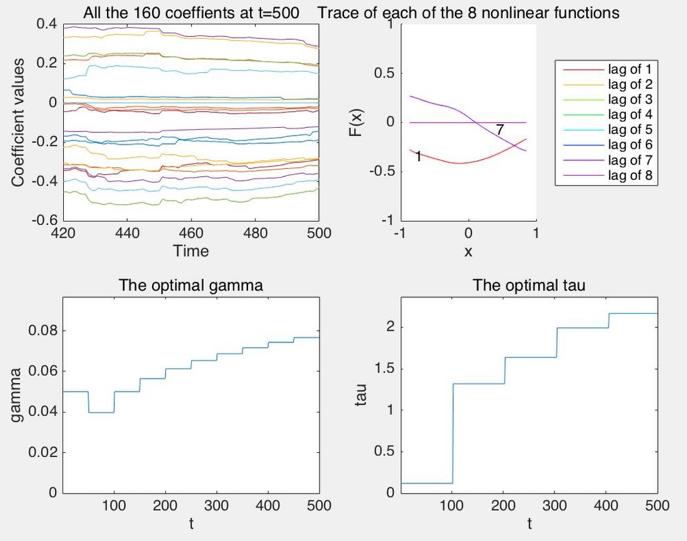
Figure 1: Four subplots show the estimated coefficients of splines, nonlinear functions, and trace plots of automatically-tuned regularization parameter $\lambda_{t}$ and innovation parameter $\tau_{t}$. A demo video is available at goo.gl/PJI2uJ

IV-A2 Synthetic data experiment: modeling nonlinear relation in adaptive environment

The purpose of this experiment is to show the performance of SLANTS in terms of prediction and nonlinearity identification when the underlying date generating model varies over time.

We have generated a synthetic data using the following nonlinear model where there is a change at time $t=500$,

$$X_{1,t} =\epsilon_{1,t},\quad X_{2,t}=0.5X_{1,t-1}^{2}-0.8X_{1,t-7}+0.2\epsilon_{2,t},\,t=1,\ldots,500,$$

$$X_{1,t} =u_{1,t},\quad X_{2,t}=-2X_{1,t-1}^{2}+\exp(X_{1,t-7})+0.2\epsilon_{2,t},\,t=501,\ldots,1000,$$

where $\epsilon_{1,t}$ and $\epsilon_{2,t}$ are i.i.d. Gaussian with mean zero and variance one. $u_{1,t}$ are i.i.d. uniform on $[-1,1]$. The initial $L$ values of $X_{2,t}$ are set to zero. The goal is to model the series $X_{2,t}$. Compared with the previous experiment, the only difference is that the forgetting factor is set to $\gamma=0.99$ in order to track potential changes in the underlying true model. Fig 2 shows that the sequential learning algorithm successfully tracked a change after the change point $t=500$. The top plot in Fig 2 shows the fit right before the change. It successfully recovers the quadratic curve of lag $1$ and linear effect of lag $7$. The bottom plot in Fig 2 shows the fit at $t=1000$. It successfully finds the exponential curve of lag $7$ and reversed sign of the quadratic curve of lag $1$. From the bottom left subplot we can see how the autotuning regularization parameter decreases since the change point $t=500$.

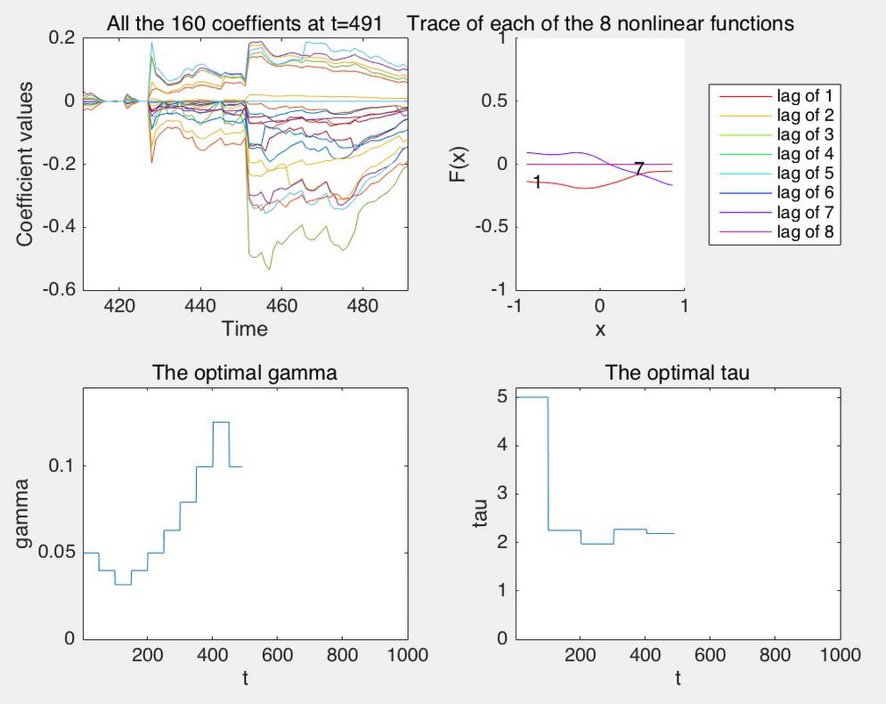
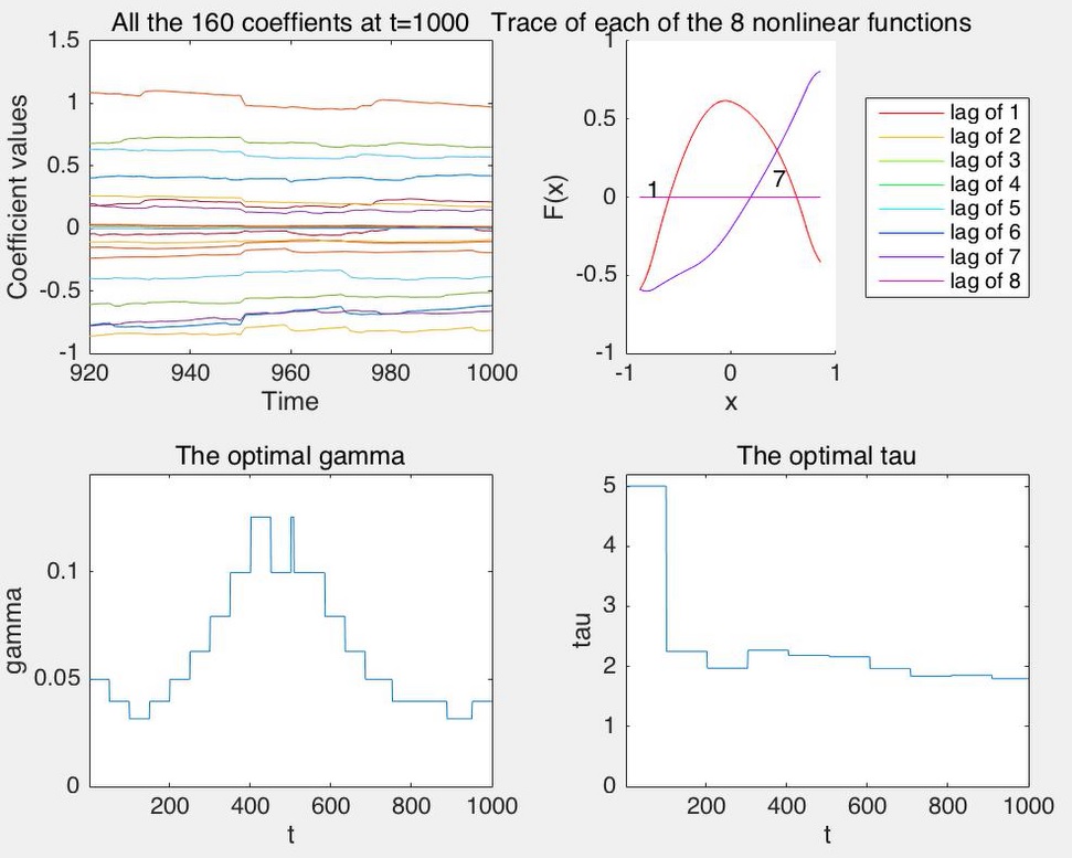
Figure 2: Two plots stacked vertically each consists of four subplots showing the estimated coefficients of splines, nonlinear functions, and trace plots of automatically-tuned regularization parameter $\lambda_{t}$ and innovation parameter $\tau_{t}$ at time $t=491$ and $t=1000$ respectively. A demo video is available at goo.gl/Vycrve

IV-A3 Synthetic data experiment: causal discovery for multi-dimensional time series

The purpose of this experiment is to show the performance of SLANTS in identifying nonlinear functional relation (thus Granger-type of causality) among multi-dimensional time series.

We have generated a 9-dimensional time series using the following nonlinear network model,

$$X_{1,t} =\epsilon_{1,t}$$

$$X_{2,t} =0.6X_{3,t-1}+\epsilon_{2,t}$$

$$X_{3,t} =0.3X_{4,t-2}^{2}+\epsilon_{3,t}$$

$$X_{4,t} =0.7X_{5,t-1}-0.2X_{5,t-2}+\epsilon_{4,t}$$

$$X_{5,t} =-0.2X_{2,t-1}^{2}+\epsilon_{5,t}$$

$$X_{6,t} =0.5X_{6,t-2}+1+\epsilon_{6,t}$$

$$X_{7,t} =2\exp(-X_{7,t-2}^{2})+\epsilon_{7,t}$$

$$X_{8,t} =6X_{7,t-1}-5X_{9,t-2}+\epsilon_{8,t}$$

$$X_{9,t} =-X_{6,t-1}+0.9X_{7,t-2}+\epsilon_{9,t}$$

where $\epsilon_{1,t}$ and $\epsilon_{2,t}$ are i.i.d. The initial $L$ values are set to zero. The goal is to model each dimension and draw sequential causality graph based on the estimation. We choose $L=2$, $M=10$ and $\gamma_{t}=1/t$. For illustration purpose, we only show the estimation for $X_{9,t}$. The left-top plot shows the 9 dimensional raw data that are sequentially obtained. The right-top plot shows the convergence of the $9\times 2\times 10=180$ coefficients in modeling $X_{9,t}$. The right-bottom plot shows how the nonlinear components $f:X_{6,t-1}\rightarrow X_{9,t}$ and $f:X_{7,t-2}\rightarrow X_{9,t}$ evolve. Similar as before, the values of each function are centralized to zero for identifiability. The left-bottom plot shows the causality graph, which is the digraph with black directed edges and edge labels indicating functional relations. For example, in modeling $X_{9,t}$, if $F(X_{6,t-1})$ is nonzero, then draw a directed graph from 6 to 9 with edge label 1; if both $F(X_{6,t-1})$ and $F(X_{6,t-2})$ are nonzero, then draw a directed graph from 6 to 9 with edge label 12. The true causality graph (determined by the above data generating process) is draw together, in red thick edges. From the simulation, the discovered causality graph quickly gets close to the truth.

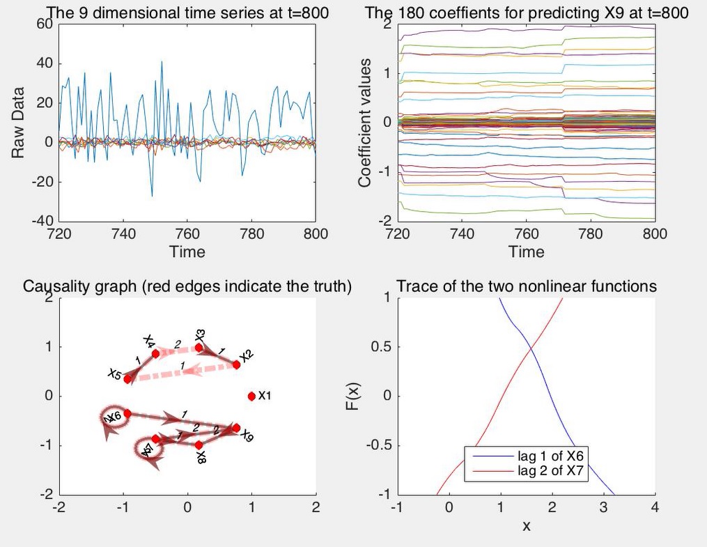
Figure 3: Four subplots show the nine time-series data, convergence of the coefficients, causality graph, and trace plot of the nonlinear functions. A demo video is available at goo.gl/sWM1oh

IV-A4 Synthetic data experiment: computation cost comparison

The purpose of this experiment is to show SLANTS is computationally efficient by comparing it to standard batch group LASSO algorithm. We use the same data generating process in the first synthetic data experiment but let the number of data points $T$ increases as $T=1000,2000,3000$. We compare to the R package ’grplasso’ [29] which implemented a widely used group LASSO algorithm. The result is shown in Table I. The table shows the time in seconds for SLANTS and grplasso to run through a dataset sequentially with different size $T$. Each run is repeated $3$ times and the standard error of running time is shown in parenthesis. From Table I, the computational cost of SLANTS grows linearly with $T$ while grplasso grows quadratically.

TABLE I: The table shows the computational cost in seconds with standard error in parenthesis for the two methods with increasing $T$.

	T=1000	T=2000	T=3000
SLANTS	24.29(0.12)	53.09(3.80)	81.36(3.42)
grplasso	25.37(0.42)	75.68(0.36)	151.41(5.58)

IV-B Real data experiment: Boston weather data from 1980 to 1986

In this experiment, we study the daily Boston weather data from 1980 Jan to 1986 Dec. with $T=2557$ points in total. The data is a six-dimensional time series, with each dimension corresponding respectively to temperature (K), relative humidity (%), east-west wind (m/s), north-south wind (m/s), sea level pressure (Pa), and precipitation (mm/day). In other words, the raw data is in the form of $X_{d,t},d=1,\ldots,6,t=1,\ldots,T$. We plot the raw data from 1980 $X_{d,t},d=1,\ldots,6,t=1,\ldots,366$ in Fig. 4.

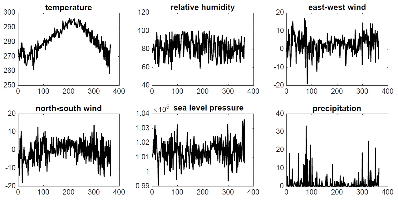
Figure 4: A graph showing the raw data of (a) temperature (K), (b) relative humidity (%), (c) east-west wind (m/s), (d) north-south wind (m/s), (e) sea level pressure (Pa), and (f) precipitation (mm/day).

We compare the predictive performance of SLANTS with that of a linear model. We chose the autoregressive model of order $3$ (denoted by AR$(3)$) as the representative linear model. The order was chosen by applying either the Akaike information criterion [30, 31] or the sample partial autocorrelations [32] to the batch data of $T$ observations. We started processing the data from $t_{0}=10$, and for each $t=t_{0}+1,\ldots,T$ the one-step ahead prediction error $\hat{e}_{t}$ was made by applying AR$(3)$ and SLANTS to the currently available $t-1$ observations. The cumulated average prediction error at time step $t$ is computed to be $\sum_{t=t_{0}+1}^{t}\hat{e}_{t}/(t-t_{0})$. Fig. 5(a). At the last time step, the significant (nonzero) functional components are the third, fourth, and sixth dimension, corresponding to EW wind, NS wind, precipitation, have been plotted in Fig. 5 (b), (c), (d), respectively. From the plot, the marginal effect of $X_{4,t}$ on $X_{3,t+1}$ is clearly nonlinear. It seems that the correlation is low for $X_{4,t}<0$ and high for $X_{4,t}>0$. In fact, if we let $\mathfrak{T}=\{t:X_{4,t}>0\}$, the correlation of $\{X_{4,t}:t\in\mathfrak{T}\}$ with $\{X_{3,t+1}:t\in\mathfrak{T}\}$ is $0.25$ (with p value $1.4\times 10^{-8}$) while $\{X_{4,t}:t\not\in\mathfrak{T}\}$ with $\{X_{3,t+1}:t\not\in\mathfrak{T}\}$ is $-0.05$ (with p value $0.24$)

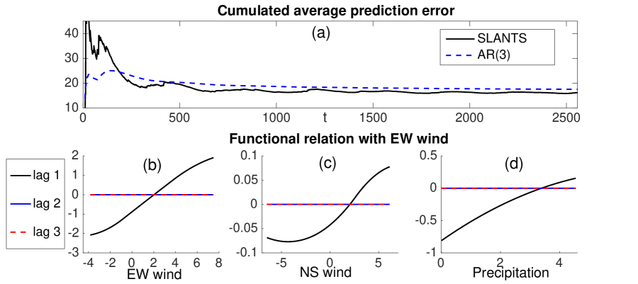
Figure 5: A graph showing (a) the cumulated average one-step ahead prediction error produced by two approaches, and east-west wind (m/s) decomposed into nonlinear functions of lagged values of (b) east-west wind, (c) north-south wind (m/s), and (c) precipitation (mm/day). The functions were output from SLANTS at the last time step $t=T$.

IV-C Real data experiment: the weekly unemployment data from 1996 to 2015

In this experiment, we study the US weekly unemployment initial claims from Jan 1996 to Dec 2015. The data is a one-dimensional time series with $T=1043$ points in total. we plot the raw data in Fig. 6.

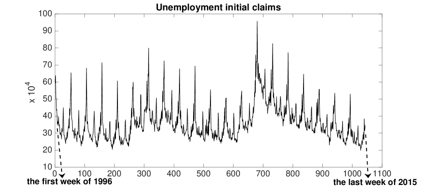
Figure 6: A graph showing the raw data of the number of unemployment initial claims.

Though the data exhibits strong cyclic pattern, it may be difficult to perform cycle-trend decomposition in a sequential environment. We explore the power of SLANTS to do lag selection to compensate the lack of such tools.

We compare three models. The first model, AR(5), is linear autoregression with lag order 5. The lag order was chosen by the sample partial autocorrelations to the batch data. The second and third are SLANTS(1) with linear spline and SLANTS(2) with quadratic splines. SLANTS(1) have 1 spline per dimension, which is exactly LASSO with auto tuning penalty parameter in SLANTS. SLANTS(2) have 8 splines per dimension. We allow SLANTS to select from a maximum lag of 55, which is roughly the size of annual cycle of 52 weeks.

Fig. 7 shows the cumulative average one-step ahead prediction error at each time step by the three approaches. Here we plot the fits to the last 800 data points due to the unstable estimates of AR and SLANTS at the beginning. The results show that SLANTS is more flexible and reliable than linear autoregressive model in practical applications. Both SLANTS(1) and SLANTS(2) selected lag 1,2,52,54 as significant predictors. It is interesting to observe that SLANTS(2) is preferred to SLANTS(1) before time step 436 (around the time when the 2008 financial crisis happened) while the simpler model SLANTS(1) is preferred after that time step. The fitted quadratic splines from SLANTS(2) are almost linear, which means the data has little nonlinearity. So SLANTS(1) performs best overall. It also demonstrates sequential LASSO as a special case of SLANTS.

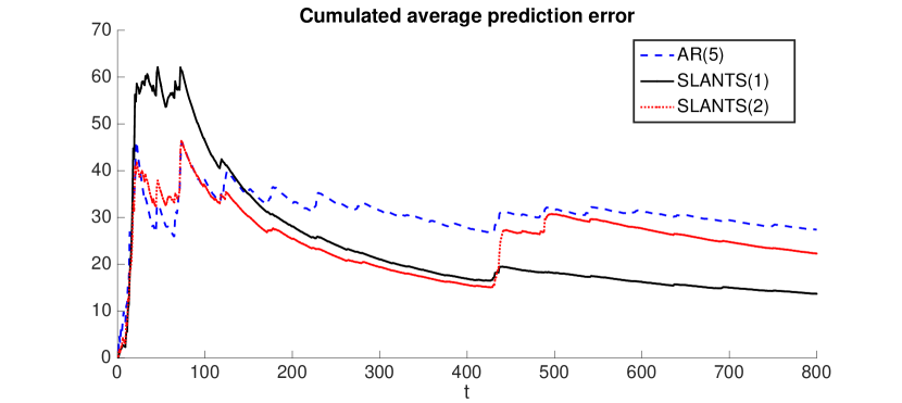
Figure 7: A graph showing the cumulative average one-step ahead prediction error at each time step produced by three approaches: linear autoregressive model, SLANTS with linear splines, and SLANTS with quadratic splines.

Appendix A Proof of Theorems

We prove Theorems 1-3 in the appendix. For any real-valued column vector $x=[x_{1},\ldots,x_{m}]$, we let $\lVert x\rVert_{2}=(\sum_{i=1}^{m}x_{i}^{2})^{1/2}$, $\lVert x\rVert_{A}=x^{\mathrm{\scriptscriptstyle T}}Ax$ denote respectively the $\ell_{2}$ norm and matrix norm (with respect to $A$, a positive semidefinite matrix).

A-A Proof of Theorem 1

At time $T$ and iteration $k$, we define the functions $h(\cdot)$ and $g(\cdot)$ that respectively map $\hat{\bm{\beta}}_{T}^{(k)}$ to $\bm{r}_{T}^{(k)}$ and from $\bm{r}_{T}^{(k)}$ to $\hat{\bm{\beta}}_{T}^{(k+1)}$, namely $\hat{\bm{\beta}}_{T}^{(k)}\xrightarrow[]{h}\bm{r}_{T}^{(k)}$, $\bm{r}_{T}^{(k)}\xrightarrow[]{g}\hat{\bm{\beta}}_{T}^{(k+1)}$. Suppose that the largest eigenvalue of $I-\tau^{2}A_{T+1}$ in absolute value is $\xi$ ($\xi<1$). In order to prove that

$$\lVert g(h(\bm{\chi}_{1}))-g(h(\bm{\chi}_{2}))\rVert_{2}\leq\xi\lVert\bm{\chi}_{1}-\bm{\chi}_{2}\rVert_{2},$$ (22)

it suffices to prove that $\lVert h(\bm{\alpha}_{1})-h(\bm{\alpha}_{2})\rVert_{2}\leq\xi\lVert\bm{\alpha}_{1}-\bm{\alpha}_{2}\rVert_{2}$ and $\lVert g(\bm{\chi}_{1})-g(\bm{\chi}_{2})\rVert_{2}\leq\lVert\bm{\chi}_{1}-\bm{\chi}_{2}\rVert_{2}$ for any vectors $\bm{\alpha}_{1},\bm{\alpha}_{2},\bm{\chi}_{1},\bm{\chi}_{2}$. The first inequality follows directly from the definition of $\bm{r}^{(k)}$ in the E step, and $h(\bm{\alpha}_{1})-h(\bm{\alpha}_{2})=(I-\tau^{2}A_{T})(\bm{\alpha}_{1}-\bm{\alpha}_{2})$. To prove the second inequality, we prove

$$\lVert g(\bm{\chi}_{1,i})-g(\bm{\chi}_{2,i})\rVert_{2}\leq\lVert\bm{\chi}_{1,i}-\bm{\chi}_{2,i}\rVert_{2},$$ (23)

where $\bm{\chi}_{k,i}$ ($i=1,\ldots,L$) are subvectors (groups ) of corresponding to $\hat{\bm{\beta}}^{(k)}_{T,i}$ for either $k=1$ or $k=2$. For brevity we define $\tilde{\tau}=\lambda_{T}\tau_{T}^{2}$. We prove (23) by considering three possible cases: 1) $\lVert\bm{\chi}_{1,i}\rVert_{2},\lVert\bm{\chi}_{2,i}\rVert_{2}\geq\tilde{\tau}$; 2) one of $\lVert\bm{\chi}_{1,i}\rVert_{2}$ and $\lVert\bm{\chi}_{2,i}\rVert_{2}$ is less than $\tilde{\tau}$ while the other is no less than $\tilde{\tau}$; 3) $\lVert\bm{\chi}_{1,i}\rVert_{2},\lVert\bm{\chi}_{2,i}\rVert_{2}<\tilde{\tau}$. For case 1), $g(\bm{\chi}_{1,i})=g(\bm{\chi}_{2,i})=\bm{0}$ and (23) trivially holds. For case 2), assume without loss of generality that $\lVert\bm{\chi}_{2,i}\rVert_{2}<\tilde{\tau}$. Then

$$\lVert g(\bm{\chi}_{1,i})-g(\bm{\chi}_{2,i})\rVert_{2} =\lVert g(\bm{\chi}_{1,i})\rVert_{2}=\lVert\bm{\chi}_{1,i}\rVert_{2}-\tilde{\tau}\leq\lVert\bm{\chi}_{1,i}\rVert_{2}-\lVert\bm{\chi}_{2,i}\rVert_{2}\leq\lVert\bm{\chi}_{1,i}-\bm{\chi}_{2,i}\rVert_{2}.$$

For case 3), we note that $g(\bm{\chi}_{k,i})$ is in the same direction of $\bm{\chi}_{k,i}$ for $k=1,2$. We define the angle between $\bm{\chi}_{1,i}$ and $\bm{\chi}_{2,i}$ to be $\theta$, and let $a=\lVert\bm{\chi}_{1,i}\rVert$, $b=\lVert\bm{\chi}_{2,i}\rVert$. By the Law of Cosines, to prove $\lVert g(\bm{\chi}_{1})-g(\bm{\chi}_{2})\rVert_{2}^{2}\leq\lVert\bm{\chi}_{1}-\bm{\chi}_{2}\rVert_{2}^{2}$ it suffices to prove that

$$(a-\tilde{\tau})^{2}+(b-\tilde{\tau})^{2}-2(a-\tilde{\tau})(b-\tilde{\tau})\cos(\theta)\leq a^{2}+b^{2}-2ab\cos(\theta).$$ (24)

By elementary calculations, Inequality (24) is equivalent to $2\{1-\cos(\theta)\}\{(a+b)\tilde{\tau}-\tilde{\tau}^{2})\}\geq 0$, which is straightforward.

Finally, Inequality (22) and Banach Fixed Point Theorem imply that

$$\lVert\hat{\bm{\beta}}_{T}^{(k)}-\hat{\bm{\beta}}_{T}\rVert_{2}\leq\frac{\xi^{k}}{1-\xi}\lVert\hat{\bm{\beta}}_{T}^{(1)}-\hat{\bm{\beta}}_{T}^{(0)}\rVert_{2}$$

which decays exponentially in $k$ for any given initial value $\hat{\bm{\beta}}_{T}^{(0)}$.

A-B Proof of Theorem 2

The proof follows standard techniques in high-dimensional regression settings [5, 28]. We only sketch the proof below. For brevity, $\hat{\bm{\beta}}_{T}$ and $\hat{\bm{\beta}}_{T,d}$ are denoted as $\hat{\bm{\beta}}$ and $\hat{\bm{\beta}}_{d}$, respectively.

Let $\tilde{S}_{1}=S_{0}\cup S_{1}$ be the set union of truly nonzero set of coefficients and the selected nonzero coefficients. By the definition of $\tilde{S}_{1}$, we have

$$\lVert Y-Z_{\tilde{S}_{1}}\hat{\bm{\beta}}_{\tilde{S}_{1}}\rVert_{2}^{2}+\tilde{\lambda}\sum\limits_{d\in\tilde{S}_{1}}\lVert\hat{\bm{\beta}}_{d}\rVert_{2}\leq\lVert Y-Z_{\tilde{S}_{1}}\bm{\beta}_{\tilde{S}_{1}}\rVert_{2}^{2}+\tilde{\lambda}\sum\limits_{d\in\tilde{S}_{1}}\lVert\bm{\beta}_{d}\rVert_{2}.$$ (25)

Define $\bm{\rho}=Y-Z\bm{\beta}$, and $\bm{\psi}=Z_{\tilde{S}_{1}}(\hat{\bm{\beta}}_{\tilde{S}_{1}}-\bm{\beta}_{\tilde{S}_{1}})$. We obtain

$$\lVert\bm{\psi}\rVert_{2}^{2} \leq 2\bm{\psi}^{\mathrm{\scriptscriptstyle T}}\bm{\rho}+\tilde{\lambda}\sum\limits_{d\in\tilde{S}_{1}}(\lVert\bm{\beta}_{d}\rVert_{2}-\lVert\hat{\bm{\beta}}_{d}\rVert_{2})$$

$$\leq 2\bm{\psi}^{\mathrm{\scriptscriptstyle T}}\bm{\rho}+\tilde{\lambda}\sum\limits_{d\in S_{0}}(\lVert\bm{\beta}_{d}\rVert_{2}-\lVert\hat{\bm{\beta}}_{d}\rVert_{2})$$

$$\leq 2\bm{\psi}^{\mathrm{\scriptscriptstyle T}}\bm{\rho}+\tilde{\lambda}\sqrt{|S_{0}|}\lVert\bm{\beta}_{\tilde{S}_{1}}-\hat{\bm{\beta}}_{\tilde{S}_{1}}\rVert_{2}$$

$$\leq 2\bm{\psi}^{\mathrm{\scriptscriptstyle T}}\bm{\rho}+\tilde{\lambda}\sqrt{|S_{1}|}\lVert\bm{\beta}_{\tilde{S}_{1}}-\hat{\bm{\beta}}_{\tilde{S}_{1}}\rVert_{2}$$

$$\leq 2\lVert\bm{\psi}\rVert_{2}\lVert\bm{\rho}\rVert_{2}+\tilde{\lambda}\sqrt{|S_{1}|}\lVert\bm{\beta}_{\tilde{S}_{1}}-\hat{\bm{\beta}}_{\tilde{S}_{1}}\rVert_{2}$$

where the first inequality is rewritten from (25), the second and fourth follow from $S_{0}\subseteq\tilde{S}_{1}$, the third and fifth follow from Cauchy inequality. From the above equality and $2\lVert\bm{\psi}\rVert_{2}\lVert\bm{\rho}\rVert_{2}\leq\lVert\bm{\psi}\rVert_{2}^{2}/2+2\lVert\bm{\rho}\rVert_{2}^{2}$, we obtain

$$\lVert\bm{\psi}\rVert_{2}^{2}\leq 4\lVert\bm{\rho}\rVert_{2}^{2}+2\tilde{\lambda}\sqrt{|S_{1}|}\lVert\bm{\beta}_{\tilde{S}_{1}}-\hat{\bm{\beta}}_{\tilde{S}_{1}}\rVert_{2}.$$ (26)

On the other hand, Assumption 4 gives $\lVert\bm{\psi}\rVert_{2}^{2}\geq\kappa T\lVert\bm{\beta}_{\tilde{S}_{1}}-\hat{\bm{\beta}}_{\tilde{S}_{1}}\rVert_{2}^{2}$. Therefore,

$$\kappa T\lVert\bm{\beta}_{\tilde{S}_{1}}-\hat{\bm{\beta}}_{\tilde{S}_{1}}\rVert_{2}^{2} \leq 4\lVert\bm{\rho}\rVert_{2}^{2}+2\tilde{\lambda}\sqrt{|S_{1}|}\lVert\bm{\beta}_{\tilde{S}_{1}}-\hat{\bm{\beta}}_{\tilde{S}_{1}}\rVert_{2}\leq 4\lVert\bm{\rho}\rVert_{2}^{2}+\frac{2\tilde{\lambda}^{2}|S_{1}|}{\kappa T}+\frac{\kappa T}{2}\lVert\bm{\beta}_{\tilde{S}_{1}}-\hat{\bm{\beta}}_{\tilde{S}_{1}}\rVert_{2}^{2}$$

which implies that

$$\lVert\bm{\beta}_{\tilde{S}_{1}}-\hat{\bm{\beta}}_{\tilde{S}_{1}}\rVert_{2}^{2}\leq 8(\kappa T)^{-1}\lVert\bm{\rho}\rVert_{2}^{2}+4(\kappa T)^{-2}\tilde{\lambda}^{2}|S_{1}|.$$ (27)

In order to bound $\lVert\bm{\beta}_{\tilde{S}_{1}}-\hat{\bm{\beta}}_{\tilde{S}_{1}}\rVert_{2}$, it remains to bound $\lVert\bm{\rho}\rVert_{2}$. Since $\rho_{t}$ can be written as

$${\varepsilon}_{t}+\sum_{d\in\tilde{S}_{1}}\{f_{d}(X_{d,t})-f^{*}_{d}(X_{d,t})\}+(\mu-\bar{Y}),$$

where $(\mu-\bar{Y})=O_{p}(T^{-1})$ and $\lVert f_{d}-f^{*}_{d}\rVert_{\infty}=O(v^{-p}+v^{1/2}T^{-1/2})$ [5, Lemma 1], we obtain $\lVert\bm{\rho}\rVert_{2}^{2}\leq 2\lVert\bm{{\varepsilon}}\rVert_{P_{X}}^{2}+c_{2}Tv^{-2p}+O_{p}(1)$ for sufficiently large $T$, where $c_{2}$ is a constant that does not depend on $v$, and $P_{X}$ is the projection matrix of $Z_{\tilde{S}_{1}}$. On the other side,

$$\lVert{\varepsilon}\rVert_{P_{X}}^{2}\leq(\kappa T)^{-1}\lVert Z_{\tilde{S}_{1}}^{\mathrm{\scriptscriptstyle T}}\bm{{\varepsilon}}\rVert_{2}^{2}.$$

Therefore,

$$\lVert\bm{\beta}_{\tilde{S}_{1}}-\hat{\bm{\beta}}_{\tilde{S}_{1}}\rVert_{2}^{2} \leq 8c_{2}\kappa^{-1}v^{-2p}+O(T^{-2}\lVert Z_{\tilde{S}_{1}}^{\mathrm{\scriptscriptstyle T}}\bm{{\varepsilon}}\rVert_{2}^{2})+O_{p}(T^{-1})+O(T^{-2}\tilde{\lambda}^{2}).$$

To finish the proof of (21), it remains to prove that $\lVert Z_{\tilde{S}_{1}}^{\mathrm{\scriptscriptstyle T}}\bm{{\varepsilon}}\rVert_{2}^{2}=O_{p}(T\log\tilde{D})$. Note that the elements of ${\varepsilon}$ are not i.i.d. conditioning on $Z_{\tilde{S}_{1}}$ due to time series dependency, which is different from the usual regression setting. However, for any of the $|S_{1}|v$ column of $Z_{\tilde{S}_{1}}$, say $\bm{z}_{d,j}$, the inner product $\bm{z}_{d,j}^{\mathrm{\scriptscriptstyle T}}\bm{{\varepsilon}}=\sum_{t=1}^{T}z_{d,j,t}{\varepsilon}_{t}$ is the sum of a martingale difference sequence (MDS) with sub-exponential condition. Applying the Bernstein-type bound for a MDS, we obtain for all $w>0$ that

$${\mathrm{pr}}\biggl{(}\biggl{|}\sum_{t=1}^{T}z_{d,j,t}{\varepsilon}_{t}\biggr{|}>w\biggr{)} \leq 2\exp\biggl{\{}-\biggl{(}2\sum_{t=1}^{T}\eta_{t}\biggr{)}^{-1}w^{2}\biggr{\}},\quad\textrm{ where }\eta_{t}\overset{\Delta}{=}var(z_{d,j,t}{\varepsilon}_{t})\leq z_{d,j,t}^{2}\sigma^{2}\leq\sup_{x\in[a,b]}\{b_{d,j}(x)\}^{2}\sigma^{2}.$$

Thus, $\sum_{t=1}^{T}z_{d,j,t}{\varepsilon}_{t}$ is a sub-Gaussian random variable for each $d,j$. By applying similar techniques used in the maximal inequality for sub-Gaussian random variables [33],

$$\max_{d\in\tilde{S}_{1},1\leq j\leq v}E(T^{-1/2}\bm{z}_{d,j}^{\mathrm{\scriptscriptstyle T}}\bm{{\varepsilon}})\leq O(T^{-\frac{1}{2}}(\log\tilde{D})^{\frac{1}{2}}).$$

Therefore,

$$\lVert Z_{\tilde{S}_{1}}^{\mathrm{\scriptscriptstyle T}}\bm{{\varepsilon}}\rVert_{2}^{2} \leq|S_{1}|vT\max_{d\in\tilde{S}_{1},1\leq j\leq v}\{E(T^{-1/2}\bm{z}_{d,j}^{\mathrm{\scriptscriptstyle T}}\bm{{\varepsilon}})\}^{2}\leq O_{p}(T\log\tilde{D}).$$

To prove $\lim_{T\rightarrow\infty}{\mathrm{pr}}(S_{0}\subseteq S_{1})=1$, we define the event $E_{0}$ as “There exists $d\in S_{0}$ such that $\hat{\bm{\beta}_{d}}=0$ and $\bm{\beta}_{d}\neq 0$”. Under event $E_{0}$, let $d$ satisfy the above requirement. Since $\lVert f_{d}-f^{*}_{d}\rVert_{\infty}=O(v^{-p}+v^{1/2}T^{-1/2})$, there exists a constant $c_{1}^{{}^{\prime}}$ such that for all $v\geq c_{1}^{{}^{\prime}}c_{0}^{-1/p}$ and sufficiently large $T$, $\lVert f^{*}_{d}\rVert_{2}\geq c_{0}/2$. By a result from [34], $\lVert\bm{\beta}_{d}\rVert_{2}^{2}/v\geq c_{2}^{{}^{\prime}}\lVert f^{*}_{d}\rVert_{2}^{2}$ holds for some constant $c_{2}^{{}^{\prime}}$. Then, under $E_{0}$ it follows that $\lVert\bm{\beta}-\hat{\bm{\beta}}\rVert_{2}^{2}\geq\lVert\bm{\beta}_{d}\rVert_{2}^{2}\geq c_{2}^{{}^{\prime}}vc_{0}^{2}/4\geq 16c_{2}v^{-2p}/\kappa$ for all $v\geq c_{1}^{{}^{\prime\prime}}c_{0}^{-2/(2p+1)}$, where $c_{1}^{{}^{\prime\prime}}$ is some positive constant. This contradicts the bound given in (21) for large $T$.

A-C Proof of Theorem 3

Recall that the backward selection procedure produces a nested sequence of subsets $S_{2}=\mathcal{S}^{(K)}\subseteq\cdots\subseteq\mathcal{S}^{(1)}\subseteq\mathcal{S}^{(0)}=S_{1}$ from sequence up to $T_{1}$ with corresponding MSE $\hat{e}^{(k)}$ ($k=0,\ldots,K$), where $0\leq K\leq|S_{1}|-|S_{2}|$. In addition, $\mathcal{S}^{(k)}=\mathcal{S}^{(k-1)}-\bar{d}_{k}^{*}$ for some $\bar{d}_{k}^{*}\in\mathcal{S}^{(k-1)}$ using theorem 2 on the sequence. It suffices to prove that as $T$ goes to infinity, with probability going to one i) $S_{0}\subseteq\mathcal{S}^{(k)}$ for each $k=0,\ldots,K$, and ii) $|S_{2}|=|S_{0}|$.

Following a similar proof by [26, Proof of Theorem 1], it can be proved that for any $k$, conditioned on $S_{0}\subseteq\mathcal{S}^{(k-1)}$, we have $\hat{e}^{(k-1)}-\hat{e}^{(k)}=O_{p}(v_{T}/T_{1})$ if $S_{0}\subseteq\mathcal{S}^{(k-1)}$, and $\hat{e}^{(k-1)}-\hat{e}^{(k)}=c+o_{p}(1)$ for some constant $c>0$ if $S_{0}\not\subseteq\mathcal{S}^{(k-1)}$. Note that the penalty increment $(v_{T}\log T_{1})/T_{1}$ is larger than $O_{p}(v_{T}/T_{1})$ and smaller than $c+o_{p}(1)$ for large $T$. By successive application of this fact finitely many times, we can prove that $S_{0}\subseteq\mathcal{S}^{(k)}$ for each $k=0,\ldots,K$, and that $|S_{2}|=|S_{0}|$ with probability close to one.

References

- [1] S. Xingjian, Z. Chen, H. Wang, D.-Y. Yeung, W.-k. Wong, and W.-c. Woo, “Convolutional lstm network: A machine learning approach for precipitation nowcasting,” in Advances in Neural Information Processing Systems, 2015, pp. 802–810.
- [2] S. Yang, M. Santillana, and S. Kou, “Accurate estimation of influenza epidemics using google search data via argo,” Proceedings of the National Academy of Sciences, vol. 112, no. 47, pp. 14 473–14 478, 2015.
- [3] S. Vijayakumar, A. D’souza, and S. Schaal, “Incremental online learning in high dimensions,” Neural computation, vol. 17, no. 12, pp. 2602–2634, 2005.
- [4] J. H. Friedman, “Multivariate adaptive regression splines,” The annals of statistics, pp. 1–67, 1991.
- [5] J. Huang, J. L. Horowitz, and F. Wei, “Variable selection in nonparametric additive models,” Annals of statistics, vol. 38, no. 4, p. 2282, 2010.
- [6] H. Tong, Threshold models in non-linear time series analysis. Springer Science & Business Media, 2012, vol. 21.
- [7] C. Gouriéroux, ARCH models and financial applications. Springer Science & Business Media, 2012.
- [8] T. J. Hastie and R. J. Tibshirani, Generalized additive models. CRC Press, 1990, vol. 43.
- [9] Z. Cai, J. Fan, and Q. Yao, “Functional-coefficient regression models for nonlinear time series,” Journal of the American Statistical Association, vol. 95, no. 451, pp. 941–956, 2000.
- [10] K. Zhang and A. Hyvärinen, “On the identifiability of the post-nonlinear causal model,” in Proceedings of the twenty-fifth conference on uncertainty in artificial intelligence. AUAI Press, 2009, pp. 647–655.
- [11] K. Zhang, J. Peters, and D. Janzing, “Kernel-based conditional independence test and application in causal discovery,” in In Uncertainty in Artificial Intelligence. Citeseer, 2011.
- [12] J. Fan, Y. Feng, and R. Song, “Nonparametric independence screening in sparse ultra-high-dimensional additive models,” Journal of the American Statistical Association, 2012.
- [13] R. Tibshirani, “Regression shrinkage and selection via the lasso,” Journal of the Royal Statistical Society. Series B (Methodological), pp. 267–288, 1996.
- [14] P. Ravikumar, J. Lafferty, H. Liu, and L. Wasserman, “Sparse additive models,” Journal of the Royal Statistical Society: Series B (Statistical Methodology), vol. 71, no. 5, pp. 1009–1030, 2009.
- [15] B. Babadi, N. Kalouptsidis, and V. Tarokh, “Sparls: The sparse rls algorithm,” Signal Processing, IEEE Transactions on, vol. 58, no. 8, pp. 4013–4025, 2010.
- [16] G. Wahba, Spline models for observational data. Siam, 1990, vol. 59.
- [17] H. Zou, “The adaptive lasso and its oracle properties,” Journal of the American statistical association, vol. 101, no. 476, pp. 1418–1429, 2006.
- [18] M. A. Figueiredo and R. D. Nowak, “An em algorithm for wavelet-based image restoration,” Image Processing, IEEE Transactions on, vol. 12, no. 8, pp. 906–916, 2003.
- [19] G. Mileounis, B. Babadi, N. Kalouptsidis, and V. Tarokh, “An adaptive greedy algorithm with application to nonlinear communications,” IEEE Transactions on Signal Processing, vol. 58, no. 6, pp. 2998–3007, 2010.
- [20] ——, “An adaptive greedy algorithm with application to sparse narma identification.” in ICASSP, 2010, pp. 3810–3813.
- [21] H. T. Friedman, J. and R. Tibshirani, “Regularization paths for generalized linear models via coordinate descent,” Journal of Statistical Software, vol. 33, no. 1, pp. 1–22, 2008.
- [22] A. P. Dawid, “Present position and potential developments: Some personal views: Statistical theory: The prequential approach,” Journal of the Royal Statistical Society. Series A (General), pp. 278–292, 1984.
- [23] T. Park and G. Casella, “The bayesian lasso,” Journal of the American Statistical Association, vol. 103, no. 482, pp. 681–686, 2008.
- [24] L. Bornn, A. Doucet, and R. Gottardo, “An efficient computational approach for prior sensitivity analysis and cross-validation,” Canadian Journal of Statistics, vol. 38, no. 1, pp. 47–64, 2010.
- [25] D. L. Jupp, “Approximation to data by splines with free knots,” SIAM Journal on Numerical Analysis, vol. 15, no. 2, pp. 328–343, 1978.
- [26] J. Z. Huang and L. Yang, “Identification of non-linear additive autoregressive models,” Journal of the Royal Statistical Society: Series B (Statistical Methodology), vol. 66, no. 2, pp. 463–477, 2004.
- [27] C. J. Stone, “Additive regression and other nonparametric models,” The annals of Statistics, pp. 689–705, 1985.
- [28] T. Hastie, R. Tibshirani, and M. Wainwright, Statistical learning with sparsity: the lasso and generalizations. CRC Press, 2015.
- [29] L. Meier, S. Van De Geer, and P. Bühlmann, “The group lasso for logistic regression,” Journal of the Royal Statistical Society: Series B (Statistical Methodology), vol. 70, no. 1, pp. 53–71, 2008.
- [30] H. Akaike, “Fitting autoregressive models for prediction,” Ann. Inst. Statist. Math., vol. 21, no. 1, pp. 243–247, 1969.
- [31] ——, “Information theory and an extension of the maximum likelihood principle,” in Selected Papers of Hirotugu Akaike. Springer, 1998, pp. 199–213.
- [32] T. Anderson, “Determination of the order of dependence in normally distributed time series,” DTIC Document, Tech. Rep., 1962.
- [33] A. W. Van Der Vaart and J. A. Wellner, Weak Convergence. Springer, 1996.
- [34] C. De Boor, C. De Boor, E.-U. Mathématicien, C. De Boor, and C. De Boor, A practical guide to splines. Springer-Verlag New York, 1978, vol. 27.