Perturbation theory for short-range weakly-attractive potentials in one dimension

Abstract

We have obtained the perturbative expressions up to sixth order for the energy of the bound state in a one dimensional, arbitrarily weak, short range finite well, applying a method originally developed by Gat and Rosenstein Ref. [3]. The expressions up to fifth order reproduce the results already known in the literature, while the sixth order had not been calculated before. As an illustration of our formulas we have applied them to two exactly solvable problems and to a nontrivial problem.

1 Introduction

We consider the Schrödinger equation in one dimension

$$\hat{H}\psi(x)=E\psi(x)$$ (1)

with

$$\hat{H}=-\frac{d^{2}}{dx^{2}}+\lambda V(x)$$ (2)

where $V(x)$ is a potential of finite depth ($\lim_{|x|\rightarrow\infty}V(x)=0$ and $V(x)<0$ for $x\in(-\infty,\infty)$).

For this problem Simon[4] has stated the necessary and sufficient conditions for a bound state to exist for $\lambda\rightarrow 0$, proving the analyticity of the lowest energy eigenvalue at $\lambda=0$, in one dimension (in two dimensions, on the other hand, Simon has also proved the non-analyticity of the eigenvalue). The work of Simon was stimulated by the findings of Abarbanel, Callan and Goldberger [5], who had obtained the expression for the lowest eigenvalue to order $\lambda^{3}$, when $V(x)$ is a short range potential. Interestingly, as mentioned by Simon in a note added in proof, the leading order term of this expansion had already been presented in the “Quantum Mechanics” book by Landau and Lifshitz [6]. More recently, Patil [7] has obtained the perturbative expression for the lowest eigenvalue to order $\lambda^{5}$ for short range potentials, using a perturbative expansion for the inverse of the T matrix, and discussed the case of long range potentials as well.

Of particular interest to the present work, is the method developed by Gat and Rosenstein in Ref. [3], which relies on an appropriate modification of the unperturbed Hamiltonian, via an attractive delta potential of arbitrarily small strength, which allows one to carry out the standard Rayleigh-Schrödinger perturbation theory; the infrared divergences, which would be present in the standard RS scheme, here identically cancel out and the result is finite when, at the end of the calculation, the strength of the delta potential is sent to zero. In this way, Gat and Rosenstein reproduced the results of Abarbanel et al.[5], obtaining the correct expression for the energy to order $\lambda^{3}$.

In the present work, we have extended the calculation of Ref. [3] to order $\lambda^{6}$, reproducing all the known results up to order $\lambda^{5}$, contained in Ref. [7], and obtaining the exact contribution of order $\lambda^{6}$, which had not been previously calculated. This work is organized as follows: in section 2 we describe the method of Gat and Rosenstein; in section 3 we work out the explicit expressions for the contributions to the energy of the ground state to fourth, fifth and sixth order in perturbation theory; in section 4 we discuss three applications of the formulas obtained in this paper; finally, in section 5 we state our conclusions. A contains the explicit expressions for the Green’s functions, appearing in the perturbative expressions.

2 The method

The first step in the application of the method is the suitable modification of the Hamiltonian, introducing a weak attractive delta potential:

$$\hat{H}=\hat{H}_{0}+\lambda V(x)$$ (3)

where

$$\hat{H}_{0}\equiv\left(-\frac{d^{2}}{dx^{2}}-2\beta\delta(x)\right)$$ (4)

is the “unperturbed hamiltonian”.

The eigenfunctions of $\hat{H}_{0}$ are

$$\psi_{0}(x) = \sqrt{\beta}e^{-\beta|x|}$$

$$\psi_{p}^{(even)}(x) = \frac{\sqrt{2}}{\sqrt{p^{2}+\beta^{2}}}\left[p\cos(px)-\beta\sin(p|x|)\right]$$

$$\psi_{p}^{(odd)}(x) = \sqrt{2}\sin(p|x|)\ .$$

and the corresponding eigenvalues are

$$\epsilon_{0} = -\beta^{2}$$

$$\epsilon_{p}^{(even)} = \epsilon_{p}^{(odd)}=p^{2}$$

In what follows we will adopt Dirac notation to denote the eigenstates of $\hat{H}_{0}$:

$$\psi_{0}(x) \rightarrow |0\rangle$$

$$\psi_{p}^{(even)}(x) \rightarrow |p^{(even)}\rangle$$

$$\psi_{p}^{(odd)}(x) \rightarrow |p^{(odd)}\rangle$$

Although the lowest orders of this expansion can be found in most books on Quantum Mechanics (ref. [6], for instance, reports the expressions up to fourth order), the higher orders must be calculated explicitly. We report the general expressions for the perturbative corrections to the energy of the ground state of Eq.(1) up to sixth order, obtained using the NCAlgebra package for Mathematica [10]:

$$E_{0}^{(1)} = \langle 0|V|0\rangle$$

$$E_{0}^{(2)} = -\langle 0|V\hat{\Omega}V|0\rangle$$

$$E_{0}^{(3)} = \langle 0|V\hat{\Omega}V\hat{\Omega}V|0\rangle-\langle 0|V|0\rangle\langle 0|V\hat{\Omega}^{2}V|0\rangle$$

$$E_{0}^{(4)} = \langle 0|V\hat{\Omega}V|0\rangle\langle 0|V\hat{\Omega}^{2}V|0\rangle+2\langle 0|V|0\rangle\langle 0|V\hat{\Omega}^{2}V\hat{\Omega}V|0\rangle$$

$$- \langle 0|V|0\rangle^{2}\langle 0|V\hat{\Omega}^{3}V|0\rangle-\langle 0|V\hat{\Omega}V\hat{\Omega}V\hat{\Omega}V|0\rangle$$

$$E_{0}^{(5)} = -\langle 0|V|0\rangle^{3}\langle 0|V\hat{\Omega}^{4}V|0\rangle$$

$$+ \langle 0|V|0\rangle^{2}\left(2\langle 0|V\hat{\Omega}^{3}V\hat{\Omega}V|0\rangle+\langle 0|V\hat{\Omega}^{2}V\hat{\Omega}^{2}V|0\rangle\right)$$

$$+ \langle 0|V|0\rangle\left(\langle 0|V\hat{\Omega}^{2}V|0\rangle^{2}-2\langle 0|V\hat{\Omega}^{2}V\hat{\Omega}V\Omega V|0\rangle+2\langle 0|V\hat{\Omega}^{3}V|0\rangle\langle 0|V\hat{\Omega}V|0\rangle-\langle 0|V\hat{\Omega}V\hat{\Omega}^{2}V\Omega V|0\rangle\right)$$

$$+ \left(-2\langle 0|V\hat{\Omega}^{2}V\hat{\Omega}V|0\rangle\langle 0|V\hat{\Omega}V|0\rangle-\langle 0|V\hat{\Omega}^{2}V|0\rangle\langle 0|V\hat{\Omega}V\hat{\Omega}V|0\rangle+\langle 0|V\hat{\Omega}V\hat{\Omega}V\Omega V\hat{\Omega}V|0\rangle\right)$$

$$E_{0}^{(6)} = -\langle 0|V|0\rangle^{4}\langle 0|V\hat{\Omega}^{5}V|0\rangle$$

$$+ 2\langle 0|V|0\rangle^{3}\left(\langle 0|V\hat{\Omega}^{4}V\hat{\Omega}V|0\rangle+\langle 0|V\hat{\Omega}^{3}V\hat{\Omega}^{2}V|0\rangle\right)$$

$$+ \langle 0|V|0\rangle^{2}\left(-2\langle 0|V\hat{\Omega}^{3}V\hat{\Omega}V\hat{\Omega}V|0\rangle+3\langle 0|V\hat{\Omega}^{3}V|0\rangle\langle 0|V\hat{\Omega}^{2}V|0\rangle-2\langle 0|V\hat{\Omega}^{2}V\hat{\Omega}^{2}V\hat{\Omega}V|0\rangle\right.$$

$$- \left.\langle 0|V\hat{\Omega}^{2}V\hat{\Omega}V\hat{\Omega}^{2}V|0\rangle+3\langle 0|V\hat{\Omega}^{4}V|0\rangle\langle 0|V\hat{\Omega}V|0\rangle-\langle 0|V\hat{\Omega}V\hat{\Omega}^{3}V\hat{\Omega}V|0\rangle\right)$$

$$- 2\langle 0|V|0\rangle\left(2\langle 0|V\hat{\Omega}^{2}V|0\rangle\langle 0|V\hat{\Omega}^{2}V\hat{\Omega}V|0\rangle-\langle 0|V\hat{\Omega}^{2}V\hat{\Omega}V\hat{\Omega}V\hat{\Omega}V|0\rangle+2\langle 0|V\hat{\Omega}^{3}V\hat{\Omega}V|0\rangle\langle 0|V\hat{\Omega}V|0\rangle\right.$$

$$+ \left.\langle 0|V\hat{\Omega}^{2}V\hat{\Omega}^{2}V|0\rangle\langle 0|V\hat{\Omega}V|0\rangle-\langle 0|V\hat{\Omega}V\hat{\Omega}^{2}V\hat{\Omega}V\hat{\Omega}V|0\rangle+\langle 0|V\hat{\Omega}^{3}V|0\rangle\langle 0|V\hat{\Omega}V\hat{\Omega}V|0\rangle\right)$$

$$+ \left(-2\langle 0|V\hat{\Omega}^{2}V\hat{\Omega}V|0\rangle-\langle 0|V\hat{\Omega}^{2}V|0\rangle\langle 0|V\hat{\Omega}V\hat{\Omega}V|0\rangle+\langle 0|V\hat{\Omega}V\hat{\Omega}V\hat{\Omega}V\hat{\Omega}V|0\rangle\right)$$

where

$$\hat{\Omega}\equiv\int_{0}^{\infty}\frac{dp}{2\pi}\frac{|p^{(even)}\rangle\langle p^{(even)}|+|p^{(odd)}\rangle\langle p^{(odd)}|}{\epsilon_{p}-\epsilon_{0}}\ .$$ (5)

Upon using the explicit expressions for the Green’s functions (reported in A) and taking the limit $\beta\rightarrow 0^{+}$ at the end of the calculation, one can obtain the exact expressions for the perturbative corrections to the energy of the ground state.

3 Perturbative calculation

The calculation of the corrections up to third order has been performed by Gat and Rosenstein in their paper [3], therefore we concentrate on the next three orders. In this section we present the calculation of the fourth, fifth and sixth orders, using the method of Gat and Rosenstein. The fourth and fifth orders obtained here reproduce the result obtained earlier by Patil, whereas the sixth order is new.

3.1 Fourth order

The direct substitution of the expressions for the Green’s functions inside the fourth order correction leads to a rather lengthy expression; it is instructive to report this expression explicitly, that reads

$$E_{0}^{(4)} = \lambda^{4}\int dx_{1}dx_{2}dx_{3}dx_{4}V(x_{1})V(x_{2})V(x_{3})V(x_{4})\frac{\left|x_{1}-x_{2}\right|+\left|x_{2}-x_{3}\right|-2\left|x_{3}-x_{4}\right|}{32\beta}$$ (6)

$$+ \lambda^{4}\int dx_{1}dx_{2}dx_{3}dx_{4}V(x_{1})V(x_{2})V(x_{3})V(x_{4})\frac{\left(-3x_{1}^{2}+6x_{2}x_{1}-8x_{2}^{2}-x_{3}^{2}+4x_{4}^{2}+10x_{2}x_{3}-8x_{3}x_{4}\right)}{64}$$

$$+ \lambda^{4}\int dx_{1}dx_{2}dx_{3}dx_{4}V(x_{1})V(x_{2})V(x_{3})V(x_{4})\mathcal{F}(x_{1},x_{2},x_{3},x_{4})$$

where

$$\mathcal{F}(x_{1},x_{2},x_{3},x_{4}) \equiv -\frac{5}{128}\left|x_{1}\right|\left|x_{1}-x_{2}\right|-\frac{5}{128}\left|x_{2}\right|\left|x_{1}-x_{2}\right|-\frac{1}{16}\left|x_{2}-x_{3}\right|\left|x_{1}-x_{2}\right|$$

$$- \frac{1}{16}\left|x_{3}\right|\left|x_{1}-x_{2}\right|-\frac{1}{16}\left|x_{3}-x_{4}\right|\left|x_{1}-x_{2}\right|-\frac{1}{16}\left|x_{4}\right|\left|x_{1}-x_{2}\right|$$

$$+ \frac{x_{2}\left|x_{1}\right|\left|x_{1}-x_{2}\right|}{128x_{1}}+\frac{x_{1}\left|x_{2}\right|\left|x_{1}-x_{2}\right|}{128x_{2}}-\frac{1}{128}\left|x_{1}\right|\left|x_{1}+x_{2}\right|$$

$$- \frac{1}{128}\left|x_{2}\right|\left|x_{1}+x_{2}\right|-\frac{1}{16}\left|x_{1}\right|\left|x_{2}-x_{3}\right|-\frac{5}{128}\left|x_{2}\right|\left|x_{2}-x_{3}\right|$$

$$- \frac{5}{128}\left|x_{2}-x_{3}\right|\left|x_{3}\right|-\frac{1}{128}\left|x_{2}\right|\left|x_{2}+x_{3}\right|-\frac{1}{128}\left|x_{3}\right|\left|x_{2}+x_{3}\right|$$

$$+ \frac{1}{8}\left|x_{1}\right|\left|x_{3}-x_{4}\right|+\frac{1}{8}\left|x_{2}\right|\left|x_{3}-x_{4}\right|-\frac{1}{16}\left|x_{2}-x_{3}\right|\left|x_{3}-x_{4}\right|$$

$$+ \frac{5}{64}\left|x_{3}\right|\left|x_{3}-x_{4}\right|-\frac{1}{16}\left|x_{2}-x_{3}\right|\left|x_{4}\right|+\frac{5}{64}\left|x_{3}-x_{4}\right|\left|x_{4}\right|$$

$$+ \frac{1}{64}\left|x_{3}\right|\left|x_{3}+x_{4}\right|+\frac{1}{64}\left|x_{4}\right|\left|x_{3}+x_{4}\right|-\frac{x_{2}\left|x_{1}\right|\left|x_{1}+x_{2}\right|}{128x_{1}}$$

$$+ \frac{x_{3}\left|x_{2}\right|\left|x_{2}-x_{3}\right|}{128x_{2}}-\frac{x_{3}\left|x_{2}\right|\left|x_{2}+x_{3}\right|}{128x_{2}}-\frac{x_{4}\left|x_{3}\right|\left|x_{3}-x_{4}\right|}{64x_{3}}$$

$$+ \frac{x_{4}\left|x_{3}\right|\left|x_{3}+x_{4}\right|}{64x_{3}}-\frac{x_{1}\left|x_{2}\right|\left|x_{1}+x_{2}\right|}{128x_{2}}+\frac{x_{2}\left|x_{2}-x_{3}\right|\left|x_{3}\right|}{128x_{3}}$$

$$- \frac{x_{2}\left|x_{3}\right|\left|x_{2}+x_{3}\right|}{128x_{3}}-\frac{x_{3}\left|x_{3}-x_{4}\right|\left|x_{4}\right|}{64x_{4}}+\frac{x_{3}\left|x_{4}\right|\left|x_{3}+x_{4}\right|}{64x_{4}}$$

It is easy to see that the infrared divergent term in the above expression, proportional to $1/\beta$, identically vanishes, appropriately relabeling the variables:

$$\int dx_{1}dx_{2}dx_{3}dx_{4}V(x_{1})V(x_{2})V(x_{3})V(x_{4})\left[\left|x_{1}-x_{2}\right|+\left|x_{2}-x_{3}\right|-2\left|x_{3}-x_{4}\right|\right]$$

$$\rightarrow \int dx_{1}dx_{2}dx_{3}dx_{4}V(x_{1})V(x_{2})V(x_{3})V(x_{4})\left[\left|x_{1}-x_{2}\right|+\left|x_{1}-x_{2}\right|-2\left|x_{1}-x_{2}\right|\right]=0$$

Let us now consider the second term, which, after a suitable relabeling reads

$$\lambda^{4}\int dx_{1}dx_{2}dx_{3}dx_{4}V(x_{1})V(x_{2})V(x_{3})V(x_{4})\frac{\left(-3x_{1}^{2}+6x_{2}x_{1}-8x_{2}^{2}-x_{3}^{2}+4x_{4}^{2}+10x_{2}x_{3}-8x_{3}x_{4}\right)}{64}$$

$$= \lambda^{4}\int dx_{1}dx_{2}dx_{3}dx_{4}V(x_{1})V(x_{2})V(x_{3})V(x_{4})\frac{x_{1}\left(x_{2}-x_{1}\right)}{8}$$

$$= \lambda^{4}\int dx_{1}dx_{2}dx_{3}dx_{4}V(x_{1})V(x_{2})V(x_{3})V(x_{4})\frac{\left(x_{2}-x_{1}\right)^{2}}{16}$$

where the last line has been obtained upon symmetrization with respect to the variables $x_{1}$ and $x_{2}$.

The simplification of the last term requires a bit more of work; the key observation is that, since $V(x_{1})V(x_{2})V(x_{3})V(x_{4})$ is completely symmetric in the variables $x_{1}$,$x_{2}$,$x_{3}$ and $x_{4}$, only the completely symmetric part of $\mathcal{F}(x_{1},x_{2},x_{3},x_{4})$ can contribute.

Upon symmetrization we obtain

$$\mathcal{F}^{({\rm sym})}(x_{1},x_{2},x_{3},x_{4}) = -\frac{1}{96}\left|x_{1}-x_{2}\right|\left|x_{1}-x_{3}\right|-\frac{1}{96}\left|x_{2}-x_{3}\right|\left|x_{1}-x_{3}\right|-\frac{1}{96}\left|x_{1}-x_{4}\right|\left|x_{1}-x_{3}\right|$$

$$- \frac{1}{48}\left|x_{2}-x_{4}\right|\left|x_{1}-x_{3}\right|-\frac{1}{96}\left|x_{3}-x_{4}\right|\left|x_{1}-x_{3}\right|-\frac{1}{96}\left|x_{1}-x_{2}\right|\left|x_{2}-x_{3}\right|$$

$$- \frac{1}{96}\left|x_{1}-x_{2}\right|\left|x_{1}-x_{4}\right|-\frac{1}{48}\left|x_{2}-x_{3}\right|\left|x_{1}-x_{4}\right|-\frac{1}{96}\left|x_{1}-x_{2}\right|\left|x_{2}-x_{4}\right|$$

$$- \frac{1}{96}\left|x_{2}-x_{3}\right|\left|x_{2}-x_{4}\right|-\frac{1}{96}\left|x_{1}-x_{4}\right|\left|x_{2}-x_{4}\right|-\frac{1}{48}\left|x_{1}-x_{2}\right|\left|x_{3}-x_{4}\right|$$

$$- \frac{1}{96}\left|x_{2}-x_{3}\right|\left|x_{3}-x_{4}\right|-\frac{1}{96}\left|x_{1}-x_{4}\right|\left|x_{3}-x_{4}\right|-\frac{1}{96}\left|x_{2}-x_{4}\right|\left|x_{3}-x_{4}\right|$$

With a suitable relabeling it is possible to reduce $\mathcal{F}^{({\rm sym})}(x_{1},x_{2},x_{3},x_{4})$ to a simpler form:

$$\mathcal{F}^{({\rm sym})}(x_{1},x_{2},x_{3},x_{4}) \rightarrow -\frac{1}{8}\left|x_{1}-x_{2}\right|\left|x_{2}-x_{3}\right|-\frac{1}{16}\left|x_{1}-x_{2}\right|\left|x_{3}-x_{4}\right|$$

Combining the contributions above one finally obtains the expression for the fourth order

$$E_{0}^{(4)} = -\frac{\lambda^{4}}{16}\left(\int V(x_{1})dx_{1}\right)^{2}\left(\int V(x_{2})|x_{2}-x_{3}|^{2}V(x_{2})dx_{2}dx_{3}\right)$$ (7)

$$- \frac{\lambda^{4}}{8}\left(\int V(x_{1})dx_{1}\right)\left(\int V(x_{2})|x_{2}-x_{3}|V(x_{3})|x_{3}-x_{4}|V(x_{4})dx_{2}dx_{3}dx_{4}\right)$$

$$- \frac{\lambda^{4}}{16}\left(\int V(x_{1})|x_{1}-x_{2}|V(x_{2})dx_{1}dx_{2}\right)^{2}$$

which agrees with the expression calculated by Patil .

3.2 Fifth order

The calculation of the higher order contributions is performed in the similar way as for the fourth order; in the case of the fifth order contribution the expression contains potentially infrared divergent terms of order $1/\beta^{3}$, $1/\beta^{2}$ and $1/\beta$. Upon symmetrization and suitable relabeling of the integration variables one can show that each of these contributions identically vanishes, as expected.

As a result, only the term of order $\beta^{0}$ survives and, upon simplification, it takes the form

$$E_{0}^{(5)} = -\frac{\lambda^{5}}{96}\left(\int V(x_{1})dx_{1}\right)^{3}\left(\int V(x_{2})|x_{2}-x_{3}|^{3}V(x_{2})dx_{2}dx_{3}\right)$$ (8)

$$- \frac{\lambda^{5}}{16}\left(\int V(x_{1})dx_{1}\right)^{2}\left(\int V(x_{2})|x_{2}-x_{3}|V(x_{3})|x_{3}-x_{4}|^{2}V(x_{4})dx_{2}dx_{3}dx_{4}\right)$$

$$- \frac{\lambda^{5}}{16}\left(\int V(x_{1})dx_{1}\right)\left(\int V(x_{2})|x_{2}-x_{3}|V(x_{3})|x_{3}-x_{4}|V(x_{4})|x_{4}-x_{5}|V(x_{5})dx_{2}dx_{3}dx_{4}dx_{5}\right)$$

$$- \frac{\lambda^{5}}{16}\left(\int V(x_{1})dx_{1}\right)\left(\int V(x_{2})|x_{2}-x_{3}|V(x_{3})dx_{2}dx_{3}\right)\left(\int V(x_{4})|x_{4}-x_{5}|^{2}V(x_{5})dx_{4}dx_{5}\right)$$

$$- \frac{\lambda^{5}}{16}\left(\int V(x_{1})|x_{1}-x_{2}|V(x_{2})dx_{1}dx_{2}\right)\left(\int V(x_{3})|x_{3}-x_{4}|V(x_{4})|x_{4}-x_{5}|V(x_{5})dx_{3}dx_{4}dx_{5}\right)$$

that agrees with the fifth order contribution calculated by Patil.

3.3 Sixth order

The calculation of the sixth order contribution is considerably more involved than the fifth order, although it can be performed along the same lines. In this case, there are divergent contributions of order $1/\beta^{4}$, $1/\beta^{3}$, $1/\beta^{2}$ and $1/\beta$. Once again, one finds that each of these contributions identically vanishes when a symmetrization of the integrands and a suitable relabeling of the integration variable is carried out.

After performing all the algebra, the simplest form that we have obtained for the sixth order term is

$$E_{0}^{(6)} = \lambda^{6}\int dx_{1}dx_{2}dx_{3}dx_{4}V(x_{1})V(x_{2})V(x_{3})V(x_{4})$$ (9)

$$\times \left(-\frac{x_{1}^{4}}{96}+\frac{1}{24}x_{2}x_{1}^{3}-\frac{5}{64}x_{2}^{2}x_{1}^{2}+\frac{3}{32}x_{2}x_{3}x_{1}^{2}-\frac{3}{64}x_{2}x_{3}x_{4}x_{1}\right)$$

$$\times \left(\int V(x_{5})dx_{5}\right)^{2}+\lambda^{6}\int dx_{1}dx_{2}dx_{3}dx_{4}dx_{5}dx_{6}V(x_{1})V(x_{2})V(x_{3})V(x_{4})V(x_{5})V(x_{6})$$

$$\times \left[\left(-\frac{1}{48}\left(x_{1}-x_{2}\right)^{2}-\frac{1}{32}\left(x_{2}-x_{3}\right)\left(x_{1}-x_{2}\right)-\frac{1}{32}\left(x_{3}-x_{4}\right)\left(x_{1}-x_{2}\right)\right.\right.$$

$$- \left.\left.\frac{1}{48}\left(x_{4}-x_{5}\right)\left(x_{1}-x_{2}\right)-\frac{1}{96}\left(x_{5}-x_{6}\right)\left(x_{1}-x_{2}\right)-\frac{1}{48}\left(x_{2}-x_{3}\right)^{2}-\frac{1}{32}\left(x_{3}-x_{4}\right)^{2}\right.\right.$$

$$- \left.\left.\frac{1}{24}\left(x_{4}-x_{5}\right)^{2}-\frac{1}{32}\left(x_{5}-x_{6}\right)^{2}-\frac{1}{32}\left(x_{2}-x_{3}\right)\left(x_{3}-x_{4}\right)\right.\right.$$

$$- \left.\left.\frac{1}{48}\left(x_{2}-x_{3}\right)\left(x_{4}-x_{5}\right)-\frac{1}{24}\left(x_{3}-x_{4}\right)\left(x_{4}-x_{5}\right)-\frac{1}{96}\left(x_{2}-x_{3}\right)\left(x_{5}-x_{6}\right)\right.\right.$$

$$- \left.\left.\frac{1}{48}\left(x_{3}-x_{4}\right)\left(x_{5}-x_{6}\right)-\frac{1}{24}\left(x_{4}-x_{5}\right)\left(x_{5}-x_{6}\right)\right)\left|x_{1}-x_{2}\right|\left|x_{2}-x_{3}\right|\right.$$

$$+ \left.\left(-\frac{1}{32}\left(x_{1}-x_{2}\right)^{2}-\frac{3}{64}\left(x_{2}-x_{3}\right)\left(x_{1}-x_{2}\right)-\frac{5}{128}\left(x_{3}-x_{4}\right)\left(x_{1}-x_{2}\right)\right.\right.$$

$$- \left.\left.\frac{1}{32}\left(x_{4}-x_{5}\right)\left(x_{1}-x_{2}\right)-\frac{1}{64}\left(x_{5}-x_{6}\right)\left(x_{1}-x_{2}\right)-\frac{3}{64}\left(x_{2}-x_{3}\right)^{2}\right.\right.$$

$$- \left.\left.\frac{1}{16}\left(x_{3}-x_{4}\right)^{2}-\frac{1}{16}\left(x_{4}-x_{5}\right)^{2}-\frac{3}{64}\left(x_{5}-x_{6}\right)^{2}\right.\right.$$

$$- \left.\left.\frac{5}{64}\left(x_{2}-x_{3}\right)\left(x_{3}-x_{4}\right)-\frac{1}{16}\left(x_{2}-x_{3}\right)\left(x_{4}-x_{5}\right)-\frac{3}{32}\left(x_{3}-x_{4}\right)\left(x_{4}-x_{5}\right)\right.\right.$$

$$- \left.\left.\frac{1}{32}\left(x_{2}-x_{3}\right)\left(x_{5}-x_{6}\right)-\frac{3}{64}\left(x_{3}-x_{4}\right)\left(x_{5}-x_{6}\right)\right.\right.$$

$$- \left.\left.\frac{1}{16}\left(x_{4}-x_{5}\right)\left(x_{5}-x_{6}\right)\right)\left|x_{1}-x_{2}\right|\left|x_{3}-x_{4}\right|\right]$$

$$+ \lambda^{6}\int dx_{1}dx_{2}dx_{3}dx_{4}dx_{5}dx_{6}V(x_{1})V(x_{2})V(x_{3})V(x_{4})V(x_{5})V(x_{6})$$

$$\times \left(-\frac{1}{32}\left|x_{1}-x_{2}\right|\left|x_{2}-x_{3}\right|\left|x_{3}-x_{4}\right|\left|x_{4}-x_{5}\right|-\frac{1}{64}\left|x_{1}-x_{2}\right|\left|x_{2}-x_{3}\right|\left|x_{5}-x_{6}\right|\left|x_{4}-x_{5}\right|\right.$$

$$- \left.\frac{1}{32}\left|x_{1}-x_{2}\right|\left|x_{2}-x_{3}\right|\left|x_{3}-x_{4}\right|\left|x_{5}-x_{6}\right|\right)\ .$$

4 Applications

We have applied this expression to two exactly solvable problems, the finite square well 

$$v(x)=\left\{\begin{array}[]{ccc}0&,&|x|>a\\ -v_{0}&,&|x|<a\end{array}\right.$$ (12)

and the Pösch-Teller potential[11]

$$v(x)=-\frac{v_{0}}{\cosh^{2}x}$$

In both cases we have reproduced the results obtained from the exact result, expanding to order $\lambda^{6}$.

For the finite square well we obtain

$$\epsilon = -v_{0}^{2}+\frac{4v_{0}^{3}}{3}-\frac{92v_{0}^{4}}{45}+\frac{1072v_{0}^{5}}{315}-\frac{84752v_{0}^{6}}{14175}+O\left(v_{0}^{7}\right)$$

whereas for the Pösch-Teller potential we obtain

$$\epsilon = -v_{0}^{2}-2v_{0}^{3}-5v_{0}^{4}-14v_{0}^{5}-42v_{0}^{6}+O\left(v_{0}^{7}\right)$$

We have also applied this formula to the case of a gaussian well

$$V(x)=-v_{0}e^{-x^{2}}$$

To order $v_{0}^{6}$ we have

$$\epsilon = -\frac{1}{4}\pi v_{0}^{2}+\frac{\pi v_{0}^{3}}{2\sqrt{2}}-\left(\frac{\pi}{8}+\frac{\sqrt{3}\pi}{8}+\frac{\pi^{2}}{12}\right)v_{0}^{4}+\left(\frac{7\pi}{96}+\frac{1}{8}\sqrt{\frac{3}{2}}\pi+\frac{3\pi^{2}}{8\sqrt{2}}+\int_{-\infty}^{\infty}F(x)dx\right)v_{0}^{5}$$ (13)

$$+ \left(-\frac{3\pi}{64}-\frac{7\pi}{96\sqrt{2}}-\frac{7\pi}{96\sqrt{5}}-\frac{5\pi^{2}}{16}-\frac{\pi^{2}}{64\sqrt{3}}-\frac{7\sqrt{3}\pi^{2}}{64}-\frac{2\pi^{3}}{45}+\int_{-\infty}^{\infty}G(x)dx\right)v_{0}^{6}+O(v_{0}^{7})$$

$$\approx -0.785398v_{0}^{2}+1.11072v_{0}^{3}-1.89534v_{0}^{4}+3.56727v_{0}^{5}-7.1374v_{0}^{6}+O(v_{0}^{7})$$

where

$$F(x) \equiv \frac{\pi^{3/2}e^{-2x^{2}}}{128}\left(e^{x^{2}}x(2{\rm erf}(x)-1)\left(4\sqrt{2}x{\rm erf}\left(\sqrt{2}x\right)-\sqrt{\pi}{\rm erf}(x)^{2}\right)-2{\rm erf}(x)^{2}\right)$$

$$G(x) \equiv \frac{\pi^{2}e^{-x^{2}}x{\rm erf}(x)^{3}}{64\sqrt{2}}+\frac{\pi^{2}e^{-x^{2}}x{\rm erf}\left(\sqrt{2}x\right){\rm erf}(x)^{2}}{32\sqrt{2}}+\frac{1}{64}\pi^{3/2}e^{-3x^{2}}{\rm erf}(x)^{2}$$

$$+ \frac{\pi^{3/2}e^{-2x^{2}}{\rm erf}(x)^{2}}{64\sqrt{2}}-\frac{1}{16}\pi^{3/2}e^{-x^{2}}x^{2}{\rm erf}\left(\sqrt{2}x\right){\rm erf}(x)-\frac{1}{16}\pi^{3/2}e^{-x^{2}}x^{2}{\rm erf}\left(\sqrt{2}x\right)^{2}$$

In this case we do not dispose of the exact result to compare with, since the problem in not exactly solvable. However, we can easily apply a Padé approximant to the perturbative expression above, after having singled out the asymptotic behavior for $v_{0}\rightarrow\infty$; the resummed expression reads

$$\tilde{\epsilon}=-v_{0}+\frac{v_{0}+2.60002v_{0}^{2}+1.2553v_{0}^{3}}{1+3.38542v_{0}+2.80348v_{0}^{2}+0.336931v_{0}^{3}}$$ (14)

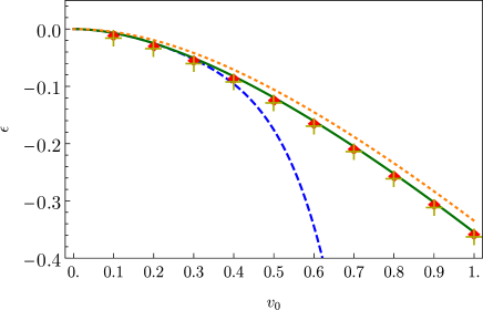
In Fig. 1 we compare the energy estimated with Eq.(14) (solid green line), with the perturbative expression to sixth order of Eq. (13) (dashed blue line), and with two variational estimates obtained with the trial wave functions

$$\psi(x)=e^{-\alpha x^{2}}$$ (15)

and

$$\psi(x)=e^{-\alpha\sqrt{\beta^{2}+x^{2}}}$$ (16)

which are respectively represented by the orange dotted line and by the red rhombi. Finally the crosses are accurate numerical results obtained by means of the Wronskian method[12].

The second wave function has the correct decay at $|x|\rightarrow\infty$: we observe an excellent agreement between the variational energy obtained in this case, minimizing with respect to the parameters $\alpha$ and $\beta$, and the energy obtained in eq. (14), using the Padé approximant of the perturbative expression to sixth order. Notice that the Padé approximant is completely analytical and does not require to introduce additional parameters.

Figure 1: Energy of the gaussian as a function of the depth. The solid green line is the Padé approximant (14), whereas the dashed blue line is the perturbative expression of eq.(13), the orange dotted line and the red rhombi are the variational energy obtained with the wave functions (15) and (16) respectively. Finally the crosses are the precise results obtained with the Wronskian method.

5 Conclusions

The calculations contained in the present paper on one hand confirm the soundness of the method originally developed by Gat and Rosenstein, reproducing the perturbative corrections to the energy of the ground state in a weak short range finite well, previously calculated with different techniques, while on another hand they provide the contribution to sixth order, which had not been calculated before. In our view, this method has the attractive feature of allowing to apply the usual Rayleigh-Schrödinger perturbation theory to a problem with a mixed (discrete-continuum) spectrum, which is intractable if one uses the free hamiltonian as the unperturbed hamiltonian $\hat{H}_{0}$, due to the presence of infrared singularities. In the scheme of Gat and Rosenstein, these singularities manifest as terms proportional to inverse powers of $\beta$ (the strength of the artificial delta potential) and turn out to exactly vanish at each perturbative order. We have applied the formula to sixth order to two exactly solvable examples, reproducing the results obtained from the exact expressions, upon expansion in the perturbative parameter. For the case of the (not-exactly solvable) gaussian well, we have compared the analytic expression obtained applying a Padé approximant to the perturbative results with the precise numerical results obtained variationally and with the method of Ref. [12], observing an excellent agreement.

Appendix A Green’s functions

In analogy with ref. [2] we define the operator

$$\hat{\Omega}_{\gamma}\equiv\int_{0}^{\infty}\frac{dp}{2\pi}\frac{|p\rangle\langle p|}{\epsilon_{p}-\epsilon_{0}+\gamma}$$ (17)

where $\epsilon_{p}=p^{2}$ and $\epsilon_{0}=-\beta^{2}$. The Dirac bra-ket notation is used for the eigenstates of $\hat{H}_{0}$ belonging to the continuum.

In terms of this operator we define the Green’s function

$$\mathcal{G}_{\gamma}(x_{1},x_{2}) \equiv \langle x_{1}|\hat{\Omega}_{\gamma}|x_{2}\rangle$$ (18)

$$= \theta\left(x_{1}\right)\theta\left(x_{1}-x_{2}\right)\theta\left(x_{2}\right)$$

$$\times \frac{e^{\left(x_{1}+x_{2}\right)(-(\beta+\Gamma))}\left(e^{\beta\left(x_{1}+x_{2}\right)}\left((\beta+1)\Gamma+\gamma\left(e^{2\Gamma x_{2}}-1\right)\right)-2\beta\Gamma e^{\Gamma\left(x_{1}+x_{2}\right)}\right)}{2\gamma\sqrt{\Gamma}}$$

$$+ \frac{\theta\left(-x_{1}\right)\theta\left(x_{1}-x_{2}\right)\theta\left(-x_{2}\right)\left(e^{\Gamma\left(x_{1}+x_{2}\right)}(\beta\Gamma-\gamma+\Gamma)-2\beta\Gamma e^{\beta\left(x_{1}+x_{2}\right)}+\gamma e^{\Gamma\left(x_{2}-x_{1}\right)}\right)}{2\gamma\sqrt{\Gamma}}$$

$$+ \frac{\sqrt{\Gamma}\theta\left(x_{1}-x_{2}\right)\theta\left(x_{1}\right)\theta\left(-x_{2}\right)e^{x_{1}(-(\beta+\Gamma))}\left(\beta\left(e^{\beta x_{1}+\Gamma x_{2}}-2e^{\beta x_{2}+\Gamma x_{1}}\right)+e^{\beta x_{1}+\Gamma x_{2}}\right)}{2\gamma}$$

$$+ \theta\left(x_{1}\right)\theta\left(x_{2}\right)\theta\left(x_{2}-x_{1}\right)$$

$$\times \frac{e^{\left(x_{1}+x_{2}\right)(-(\beta+\Gamma))}\left(\gamma e^{\beta\left(x_{1}+x_{2}\right)+2\Gamma x_{1}}+e^{\beta\left(x_{1}+x_{2}\right)}(\beta\Gamma-\gamma+\Gamma)-2\beta\Gamma e^{\Gamma\left(x_{1}+x_{2}\right)}\right)}{2\gamma\sqrt{\Gamma}}$$

$$+ \frac{\theta\left(-x_{1}\right)\theta\left(-x_{2}\right)\theta\left(x_{2}-x_{1}\right)\left(e^{\Gamma\left(x_{1}+x_{2}\right)}(\beta\Gamma-\gamma+\Gamma)-2\beta\Gamma e^{\beta\left(x_{1}+x_{2}\right)}+\gamma e^{\Gamma\left(x_{1}-x_{2}\right)}\right)}{2\gamma\sqrt{\Gamma}}$$

$$+ \frac{\sqrt{\Gamma}\theta\left(-x_{1}\right)\theta\left(x_{2}\right)\theta\left(x_{2}-x_{1}\right)\left(\beta\left(e^{\Gamma\left(x_{1}-x_{2}\right)}-2e^{\beta\left(x_{1}-x_{2}\right)}\right)+e^{\Gamma\left(x_{1}-x_{2}\right)}\right)}{2\gamma}$$

where

$$\Gamma\equiv\sqrt{\beta^{2}+\gamma}$$ (19)

We have

$$\mathcal{G}_{\gamma}(x_{1},x_{2})=\sum_{\ell=0}^{\infty}(-1)^{\ell}\mathcal{G}^{(\ell)}(x_{1},x_{2})$$ (20)

where

$$\mathcal{G}^{(\ell)}(x_{1},x_{2})=\langle x_{1}|\hat{\Omega}^{\ell+1}|x_{2}\rangle$$ (21)

are the Green’s functions needed in the application of the perturbative method.

The explicit expressions for the first few Green’s functions are

$$\mathcal{G}^{(0)}(x_{1},x_{2}) = \frac{1}{4\beta}+\frac{1}{4}\left(-\left|x_{1}\right|-2\left|x_{1}-x_{2}\right|-\left|x_{2}\right|\right)+O(\beta)$$

$$\mathcal{G}^{(1)}(x_{1},x_{2}) = \frac{1}{16\beta^{3}}-\frac{\left|x_{1}\right|+\left|x_{2}\right|}{16\beta^{2}}+\frac{2\left|x_{1}\right|\left|x_{2}\right|-3x_{1}^{2}+8x_{1}x_{2}-3x_{2}^{2}}{32\beta}$$

$$+ \frac{1}{96}\left(8\left|x_{1}-x_{2}\right|\left(x_{1}-x_{2}\right)^{2}+3\left|x_{2}\right|\left(3x_{1}^{2}+x_{2}^{2}\right)+3\left|x_{1}\right|\left(x_{1}^{2}+3x_{2}^{2}\right)\right)+O(\beta)$$

$$\mathcal{G}^{(2)}(x_{1},x_{2}) = \frac{1}{32\beta^{5}}-\frac{\left|x_{1}\right|+\left|x_{2}\right|}{32\beta^{4}}-\frac{-2\left|x_{1}\right|\left|x_{2}\right|+x_{1}^{2}-4x_{1}x_{2}+x_{2}^{2}}{64\beta^{3}}$$

$$+ \frac{\left(\left|x_{1}\right|+3\left|x_{2}\right|\right)x_{1}^{2}+\left(3\left|x_{1}\right|+\left|x_{2}\right|\right)x_{2}^{2}}{192\beta^{2}}$$

$$+ \frac{5x_{1}^{4}-24x_{1}^{3}x_{2}+30x_{1}^{2}x_{2}^{2}-24x_{1}x_{2}^{3}+5x_{2}^{4}-4\left|x_{1}\right|\left|x_{2}\right|\left(x_{1}^{2}+x_{2}^{2}\right)}{768\beta}$$

$$+ \frac{-16\left|x_{1}-x_{2}\right|\left(x_{1}-x_{2}\right)^{4}-5\left|x_{2}\right|\left(5x_{1}^{4}+10x_{1}^{2}x_{2}^{2}+x_{2}^{4}\right)-5\left|x_{1}\right|\left(x_{1}^{4}+10x_{1}^{2}x_{2}^{2}+5x_{2}^{4}\right)}{3840}+O(\beta)$$

$$\mathcal{G}^{(3)}(x_{1},x_{2}) = \frac{5}{256\beta^{7}}-\frac{5\left(\left|x_{1}\right|+\left|x_{2}\right|\right)}{256\beta^{6}}+\frac{10\left|x_{1}\right|\left|x_{2}\right|-3x_{1}^{2}+16x_{1}x_{2}-3x_{2}^{2}}{512\beta^{5}}$$ (22)

$$+ \frac{\left(\left|x_{1}\right|+3\left|x_{2}\right|\right)x_{1}^{2}+\left(3\left|x_{1}\right|+\left|x_{2}\right|\right)x_{2}^{2}}{512\beta^{4}}$$

$$+ \frac{5x_{1}^{4}-32x_{1}^{3}x_{2}+30x_{1}^{2}x_{2}^{2}-32x_{1}x_{2}^{3}+5x_{2}^{4}-12\left|x_{1}\right|\left|x_{2}\right|\left(x_{1}^{2}+x_{2}^{2}\right)}{6144\beta^{3}}$$

$$- \frac{\left(\left|x_{1}\right|+5\left|x_{2}\right|\right)x_{1}^{4}+10\left(\left|x_{1}\right|+\left|x_{2}\right|\right)x_{1}^{2}x_{2}^{2}+\left(5\left|x_{1}\right|+\left|x_{2}\right|\right)x_{2}^{4}}{6144\beta^{2}}$$

$$+ \frac{1}{36864\beta}\left[-7x_{1}^{6}+48x_{1}^{5}x_{2}-105x_{1}^{4}x_{2}^{2}+160x_{1}^{3}x_{2}^{3}-105x_{1}^{2}x_{2}^{4}+48x_{1}x_{2}^{5}\right.$$

$$- \left.7x_{2}^{6}+2\left|x_{1}x_{2}\right|\left(3x_{1}^{2}+x_{2}^{2}\right)\left(x_{1}^{2}+3x_{2}^{2}\right)\right]$$

$$+ \frac{1}{1290240}\left[128\left|x_{1}-x_{2}\right|\left(x_{1}-x_{2}\right)^{6}\right.$$

$$+ \left.35\left|x_{2}\right|\left(7x_{1}^{6}+35x_{1}^{4}x_{2}^{2}+21x_{1}^{2}x_{2}^{4}+x_{2}^{6}\right)+35\left|x_{1}\right|\left(x_{1}^{6}+21x_{1}^{4}x_{2}^{2}+35x_{1}^{2}x_{2}^{4}+7x_{2}^{6}\right)\right]$$

$$+ O(\beta)$$

References

- [1] P. Amore, F.M.Fernández and C.P. Hofmann, European Physical Journal B 89, 163 (2016)
- [2] P. Amore, ”Weakly bound states in heterogeneous waveguides: a calculation to fourth order”, arXiv:1601.02470 (2016)
- [3] G. Gat, B. Rosenstein, Phys. Rev. Lett. 70 (1993) 5.
- [4] B. Simon, Annals of Physics 97, 279-288 (1976)
- [5] H. Abarbanel, C. Callan and M. Goldberger, unpublished (1976)
- [6] Landau and Lifshitz, Quantum mechanics, Pergamon Press
- [7] S.H. Patil, Phys. Rev. A 22, 1655-1663 (1980)
- [8] S.H. Patil, Phys. Rev. A 22, 2400-2402 (1980)
- [9] S.H. Patil, Phys. Rev. A 25, 2467-2472 (1982)
- [10] http://math.ucsd.edu/ ncalg/
- [11] S. Flügge, Practical Quantum Mechanics, Springer-Verlag, Berlin, 1999).
- [12] F. M. Fernández,Eur. J. Phys. 32, 723-732 (2011)