Efficient transfer of an arbitrary qutrit state in circuit QED

Abstract

Compared with a qubit, a qutrit (i.e., three-level quantum system) has a larger Hilbert space and thus can be used to encode more information in quantum information processing and communication. Here, we propose a method to transfer an arbitrary quantum state between two flux qutrits coupled to two resonators. This scheme is simple because it only requires two basic operations. The state-transfer operation can be performed fast because of using resonant interactions only. Numerical simulations show that high-fidelity transfer of quantum states between the two qutrits is feasible with current circuit-QED technology. This scheme is quite general and can be applied to accomplish the same task for other solid-state qutrits coupled to resonators.

Superconducting qubits for quantum information and quantum computation have attracted considerable attention due to their controllability, ready fabrication, integrability, and potential scalability [1-5]. Their coherence time has recently been significantly increased [6-11]. For superconducting qubits, the level spacings can be rapidly adjusted within 1-3 ns, by varying external control parameters (e.g., magnetic flux applied to the superconducting loop of a superconducting phase, transmon, Xmon or flux qubit; see, e.g., [8,12-14]). In addition, circuit QED, i.e., analogs of cavity QED with solid-state systems, has been considered as one of the most promising candidates for building quantum computers and quantum information processors [3-5,15,16]. Furthermore, the strong-coupling or ultrastrong-coupling regime of a qubit with a microwave cavity has been reported in experiments [17,18].

Quantum information processing (QIP) with qudits ($d$-level systems), including qutrits, has been attracting increasing interest. For example, QIP and tomography of nanoscale semiconductor devices were studied (see, Refs. [19,20] and references therein). On the other hand, quantum state transfer (QST) plays an important role in quantum communication and QIP. Over the past years, theoretical proposals have been presented for realizing qubit-to-qubit QST with two superconducting qubits, which are coupled through a cavity/resonator [21-28] or a capacitor [29]. The cavity/resonator acts as a quantum data bus to mediate long-range and fast interaction between superconducting qubits. The QST between two superconducting qubits has been demonstrated in circuits consisting of superconducting qubits coupled to cavities or resonators [30-33]. However, to the best of our knowledge, there is no study of qutrit-to-qutrit QST in circuit QED.

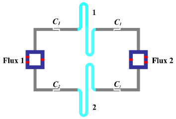
Figure 1: Diagram of a setup for two flux qutrits coupled to two TLRs via capacitances $C_{1}$ and $C_{2}$. A blue square represents a flux qutrit, which can be other types of solid-state qutrit, such as a quantum dot, a superconducting phase qutrit or a transmon qutrit.

In this letter, we propose a scheme to transfer an arbitrary quantum state between two superconducting flux qutrits, coupled to two transmission line resonators (TLRs) (Fig. 1). The three levels of qutrit $j$ are denoted as $|g\rangle_{j},$ $|e\rangle_{j},$ and $|f\rangle_{j}$ $(j=1,2)$ (Fig. 2). The QST from qutrit 1 to qutrit 2 is expressed by the formula

$$(\alpha|g\rangle_{1}+\beta|e\rangle_{1}+\gamma|f\rangle_{1})|g\rangle_{2}$$

$$\rightarrow|g\rangle_{1}(\alpha|g\rangle_{2}+\beta|e\rangle_{2}+\gamma|f\rangle_{2}),$$ (1)

where $\alpha,$ $\beta,$ and $\gamma$ are the normalized complex numbers; the subscripts 1 and 2 represent qutrit 1 and qutrit 2.

This scheme has the following advantages. Firstly, it is simple because the state transfer requires only two basic operations. Secondly, the speed of operation is fast because of using resonant interactions, e.g., the QST can be completed within $\sim 8.5$ ns, as shown in our following numerical simulation. Thirdly, through the numerical simulation, we find that precise control of qutrit-resonator coupling and qutrit-resonator resonance is not necessary and the qutrit-to-qutrit QST with a high fidelity is feasible with current circuit-QED technology. Lastly, this scheme is quite general and can be applied to implement QST between other solid-state qutrits, e.g., other types of superconducting qutrits or quantum dots coupled to resonators. We hope this work will stimulate experimental activities in the near future.

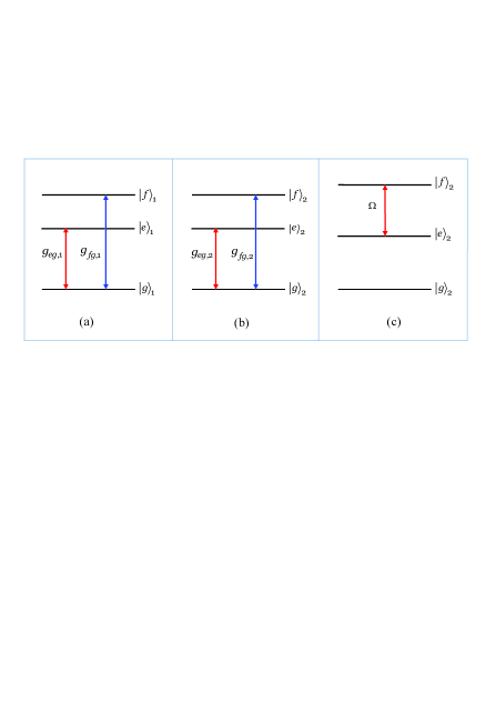
Figure 2: (a) TLR 1 (2) is resonant with the $|g\rangle\leftrightarrow|e\rangle$ ($|g\rangle\leftrightarrow|f\rangle$) transition of qutrit 1 with a coupling constant $g_{eg,_{1}}$ ($g_{fg,_{1}}$). (b) TLR 1 (2) is resonant with $|g\rangle\leftrightarrow|e\rangle$ ($|g\rangle\leftrightarrow|f\rangle$) transition of qutrit 2 with a coupling constant $g_{eg,_{2}}$ ($g_{fg,_{2}}$). (c) The classical pulse is resonant with the $|e\rangle\leftrightarrow|f\rangle$ transition of qutrit 2, with a Rabi frequency $\Omega$.

Consider a system of two flux qutrits connected by two TLRs (Fig. 1). As shown in Fig. 2(a,b), TLR 1 is resonantly coupled to the $|g\rangle\leftrightarrow|e\rangle$ transition of qutrit $j$ with a coupling constant $g_{eg,_{j}}$, TLR 2 is resonantly coupled to the $|g\rangle\leftrightarrow|f\rangle$ transition of qutrit $j$ with a coupling constant $g_{fg,_{j}}$ $(j=1,2)$. In the interaction picture, the Hamiltonian is given by (in units of $\hbar=1$)

$$H_{I_{,}1} = \sum_{j=1}^{2}g_{eg,_{j}}(a_{1}\sigma_{eg,_{j}}^{+}+h.c.)$$ (2)

$$+ \sum_{j=1}^{2}g_{fg,_{j}}(a_{2}\sigma_{fg,_{j}}^{+}+h.c.),$$

where $a_{j}$ is the photon annihilation operator for the TLR $j$, $\sigma_{eg,_{j}}^{+}=|e\rangle_{j}\langle g|$ and $\sigma_{fg,_{j}}^{+}=|f\rangle_{j}\langle g|$ $(j=1,2)$. For simplicity, we set $g_{eg,j}=g_{fg,_{j}}\equiv g$, which can be achieved by a prior design of the sample with appropriate capacitances $C_{1}$ and $C_{2}$.

Under the Hamiltonian (2), one can obtain the following state evolutions

$$|g\rangle|0\rangle|0\rangle|g\rangle \rightarrow |g\rangle|0\rangle|0\rangle|g\rangle,$$

$$|e\rangle|0\rangle|0\rangle|g\rangle \rightarrow \frac{1}{2}(1+\cos\sqrt{2}gt)|e\rangle|0\rangle|0\rangle|g\rangle$$

$$- \frac{\sqrt{2}}{2}i\sin(\sqrt{2}gt)|g\rangle|1\rangle|0\rangle|g\rangle$$

$$- \frac{1}{2}(1-\cos\sqrt{2}gt)|g\rangle|0\rangle|0\rangle|e\rangle,$$

$$|f\rangle|0\rangle|0\rangle|g\rangle \rightarrow \frac{1}{2}(1+\cos\sqrt{2}gt)|f\rangle|0\rangle|0\rangle|g\rangle$$ (3)

$$- \frac{\sqrt{2}}{2}i\sin(\sqrt{2}gt)|g\rangle|0\rangle|1\rangle|g\rangle$$

$$- \frac{1}{2}(1-\cos\sqrt{2}gt)|g\rangle|0\rangle|0\rangle|f\rangle.$$

Here and below, the left $|0\rangle$ ($|1\rangle$) in each term represents the vacuum state (the single photon state) of TLR 1 while the right $|0\rangle$ ($|1\rangle$) in each term represents the vacuum state (the single photon state) of TLR 2; in addition, the left $|g\rangle$, $|e\rangle$, and $|f\rangle$ in each term are the states of qutrit 1 while the right $|g\rangle$, $|e\rangle$, and $|f\rangle$ in each term are the states of qutrit 2.

From Eq. (3), it can be seen that when the interaction time is equal to $t_{1}=\pi/(\sqrt{2}g)$, one obtains the transformations $|g\rangle|0\rangle|0\rangle|g\rangle\rightarrow|g\rangle|0\rangle|0\rangle|g\rangle$, $|e\rangle|0\rangle|0\rangle|g\rangle\rightarrow-|g\rangle|0\rangle|0\rangle|e\rangle$, $|f\rangle|0\rangle|0\rangle|g\rangle\rightarrow-|g\rangle|0\rangle|0\rangle|f\rangle$ simultaneously. As a result, we have the following state transformation

$$(\alpha|g\rangle+\beta|e\rangle+\gamma|f\rangle)|0\rangle|0\rangle|g\rangle$$

$$\rightarrow|g\rangle|0\rangle|0\rangle(\alpha|g\rangle-\beta|e\rangle-\gamma|f\rangle).$$ (4)

Adjust the level spacings of each qutrit so that it is decoupled from the two TLRs. Then apply a classical pulse to qutrit 2. The pulse is resonant with the $|e\rangle\leftrightarrow|f\rangle$ transition of qutrit 2 [Fig. 2(c)]. The Hamiltonian in the interaction picture is expressed as

$$H_{I_{,}2}=\Omega(|e\rangle_{2}\langle f|+h.c.),$$ (5)

where $\Omega$ is the Rabi frequency of the pulse. One can obtain the following rotations under the Hamiltonian (5),

$$|e\rangle_{2} \rightarrow \cos(\Omega t)|e\rangle_{2}-i\sin(\Omega t)|f\rangle_{2},$$

$$|f\rangle_{2} \rightarrow \cos(\Omega t)|f\rangle_{2}-i\sin(\Omega t)|e\rangle_{2}.$$ (6)

We set $t_{2}=\pi/\Omega$ to obtain a $\pi$ rotation by $|e\rangle_{2}\rightarrow-|e\rangle_{2}$ and $|f\rangle_{2}\rightarrow-|f\rangle_{2}$. Hence, we can obtain $-|g\rangle|0\rangle|0\rangle|e\rangle\rightarrow|g\rangle|0\rangle|0\rangle|e\rangle$ and $-|g\rangle|0\rangle|0\rangle|f\rangle\rightarrow|g\rangle|0\rangle|0\rangle|f\rangle$. Therefore, it follows from Eq. (4)

$$(\alpha|g\rangle+\beta|e\rangle+\gamma|f\rangle)|0\rangle|0\rangle|g\rangle$$

$$\rightarrow|g\rangle|0\rangle|0\rangle(\alpha|g\rangle+\beta|e\rangle+\gamma|f\rangle),$$ (7)

which shows that the original state of qutrit 1 is perfectly transferred to qutrit 2 after the above operation.

Let us now give a discussion of the experimental implementation. For a general consideration, we will analyze the fidelity of the QST by allowing a small qutrit-resonator frequency detuning. In addition, we take into account the crosstalk between the two resonators. Thus, the Hamiltonian (2) is modified as follows

$$\widetilde{H}_{I,1} = \sum_{j=1}^{2}g_{eg,_{j}}(e^{i\delta_{1}t}a_{1}\sigma_{eg,_{j}}^{+}+h.c.)$$ (8)

$$+ \sum_{j=1}^{2}g_{fg,_{j}}(e^{i\delta_{2}t}a_{2}\sigma_{fg,_{j}}^{+}+h.c.)$$

$$+ g_{12}\left(e^{i\Delta t}a_{1}a_{2}^{\dagger}+h.c.\right).$$

The first (second) term of Eq. (8) describes the coupling between TLR 1 (2) and the $\left|g\right\rangle\leftrightarrow\left|e\right\rangle$ ($\left|g\right\rangle\leftrightarrow\left|f\right\rangle)$ transition of qutrit $j$, with detuning $\delta_{1}=\omega_{eg_{j}}-\omega_{c_{1}}$ ($\delta_{2}=\omega_{fg_{j}}-\omega_{c_{2}}$). Here, $\omega_{eg_{j}}$ ($\omega_{fg_{j}}$) is the $\left|g\right\rangle\leftrightarrow\left|e\right\rangle$ ($\left|g\right\rangle\leftrightarrow\left|f\right\rangle)$ transition frequency of qutrit $j$, and $\omega_{c_{j}}$ is the frequency of TLR $j$ $(j=1,2)$. For simplicity, we consider identical flux qutrits and set $\delta_{1}=\delta_{2}=\delta$. The last term of Eq. (8) describes the inter-resonator crosstalk between the two TLRs, where $\Delta=\omega_{c_{2}}-\omega_{c_{1}}$ is detuning between the two-TLR frequencies and $g_{12}$ is the inter-resonator crosstalk coupling strength.

We also consider the inter-resonator crosstalk coupling during the qutrit-pulse resonant interaction. Thus, the Hamiltonian (5) is modified as

$$\widetilde{H}_{I,2}=H_{I,2}+g_{12}\left(e^{i\Delta t}a_{1}a_{2}^{\dagger}+h.c.\right).$$ (9)

The dynamics of the lossy system, with finite qutrit relaxation and dephasing and photon lifetime included, is determined by the following master equation

$$\frac{d\rho}{dt} = -i[\widetilde{H}_{I},\rho]+\sum_{j=1}^{2}\kappa_{j}\mathcal{L}[a_{j}]$$ (10)

$$+ \sum_{j=1,2}\left\{\gamma_{eg_{j}}\mathcal{L}[\sigma_{eg,_{j}}^{-}]+\gamma_{fe_{j}}\mathcal{L}[\sigma_{fe,_{j}}^{-}]+\gamma_{fg_{j}}\mathcal{L}[\sigma_{fg,_{j}}^{-}]\right\}$$

$$+ \sum_{j=1,2}\left\{\gamma_{j,\varphi f}\left(\sigma_{ff_{j}}\rho\sigma_{ff_{j}}-\sigma_{ff_{j}}\rho/2-\rho\sigma_{ff_{j}}/2\right)\right\}$$

$$+ \sum_{j=1,2}\left\{\gamma_{j,\varphi e}\left(\sigma_{ee_{j}}\rho\sigma_{ee_{j}}-\sigma_{ee_{j}}\rho/2-\rho\sigma_{ee_{j}}/2\right)\right\},$$

where $\widetilde{H}_{I}$ is $\widetilde{H}_{I,1}$ or $\widetilde{H}_{I,2}$ above, $\sigma_{eg,_{j}}^{-}=\left|g\right\rangle_{j}\left\langle e\right|$, $\sigma_{fe,_{j}}^{-}=\left|e\right\rangle_{j}\left\langle f\right|$, $\sigma_{fg,_{j}}^{-}=\left|g\right\rangle_{j}\left\langle f\right|,\sigma_{ee_{j}}=\left|e\right\rangle_{j}\left\langle e\right|,\sigma_{ff_{j}}=\left|f\right\rangle_{j}\left\langle f\right|;$ and $\mathcal{L}\left[\Lambda\right]=\Lambda\rho\Lambda^{+}-\Lambda^{+}\Lambda\rho/2-\rho\Lambda^{+}\Lambda/2,$ with $\Lambda=a_{j},\sigma_{eg,_{j}}^{-},\sigma_{fe,_{j}}^{-},\sigma_{fg,_{j}}^{-}.$ Here, $\kappa_{j}$ is the photon decay rate of TLR $j$. In addition, $\gamma_{eg_{j}}$ is the energy relaxation rate of the level $\left|e\right\rangle$ of qutrit $j$, $\gamma_{fe_{j}}$ ($\gamma_{fg_{j}}$) is the energy relaxation rate of the level $\left|f\right\rangle$ of qutrit $j$ for the decay path $\left|f\right\rangle\rightarrow\left|e\right\rangle$ ($\left|g\right\rangle$), and $\gamma_{j,\varphi e}$ ($\gamma_{j,\varphi f}$) is the dephasing rate of the level $\left|e\right\rangle$ ($\left|f\right\rangle$) of qutrit $j$ ($j=1,2$).

The fidelity of the operation is given by $\mathcal{F}=\sqrt{\left\langle\psi_{\mathrm{id}}\right|\rho\left|\psi_{\mathrm{id}}\right\rangle},$ where $\left|\psi_{\mathrm{id}}\right\rangle$ is the output state $|g\rangle|0\rangle|0\rangle(\alpha|g\rangle+\beta|e\rangle+\gamma|f\rangle)$ of an ideal system (i.e., without dissipation, dephasing, and crosstalk); while $\rho$ is the final density operator of the system when the operation is performed in a realistic situation. As an example, we will consider the case of $\alpha=\beta=\gamma=1/\sqrt{3}$ in the following analysis.

We now numerically calculate the fidelity of operation. We set $\Omega/2\pi=$100 MHz, which can be achieved in experiments [34]. For a flux qutrit, the transition frequency between two neighbor levels is 1 to 30 GHz. Thus, we can choose $\omega_{c_{1}}/2\pi=4.5$ GHz and $\omega_{c_{2}}/2\pi=7.0$ GHz. Accordingly, we have $\Delta/2\pi=2.5$ GHz. We assume that the frequencies of the TLRs are fixed during the entire operation. Other parameters used in the numerical simulation are: (i) $\gamma^{-1}_{j,\varphi e}=1.5~{}\mu s,$ $\gamma^{-1}_{j,\varphi f}=0.5~{}\mu s$; (ii) $\gamma^{-1}_{eg_{j}}=\gamma^{-1}_{fe_{j}}=\gamma^{-1}_{fg_{j}}=2.5~{}\mu s$; (iii) $\kappa^{-1}_{j}=20~{}\mu s$ $(j=1,2)$. We here consider a conservative case for the decoherence times of flux qutrits [11].

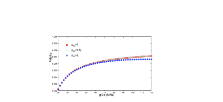
Figure 3: Fidelity versus $g/2\pi$, plotted for $g_{eg,j}=g_{fg,_{j}}\equiv g$ ($j=1,2$); $g_{12}=0,0.1g,g$; and $\delta=0$ (i.e., the qutrit-resonator resonance case). Here and in Fig. 4, $g_{12}$ is the inter-resonator crosstalk coupling strength and $\delta$ is the detuning.

To start with, let us first investigate the effect of the inter-resonator crosstalk on the operational fidelity. Figure 3 depicts the fidelity versus $g/2\pi$ with $g_{12}=0,0.1g,g$, which is plotted for the qutrit-resonator resonance case. From Fig. 3, one can see that the effect of the inter-resonator crosstalk is very small when $g_{12}\leq 0.1g$ and a high fidelity $\sim 99.7\%$ can be reached for $g/2\pi=100$ MHz [18]. In this case, the estimated operation time is $\sim 8.5$ ns. In the following, we choose $g_{12}=0.1g$, which is readily satisfied in experiments  [35].

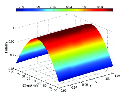
Figure 4: Fidelity versus $\delta/2\pi$ and $c$, plotted for $g_{12}=0.1g$ and $g/2\pi=100$ MHz. Here, $c=g_{fg,_{j}}/g_{eg,j}$, with $g_{eg,j}\equiv g$ ($j=1,2$).

In realistic situation, it may be a challenge to obtain exact qutrit-resonator resonant interaction and identical qutrit-resonator coupling. Thus, we consider a small qutrit-resonator frequency detuning and inhomogeneous qutrit-resonator coupling. We set $g_{eg,1}=g_{eg,2}=g$ but $g_{fg,_{1}}=g_{fg,_{2}}=cg$, with $c\in[0.95,1.05]$. This may apply when the two qutrits $1$ and $2$, the two coupling capacitances $C_{1}$ (Fig.1), and the two coupling capacitances $C_{2}$ (Fig. 1) are approximately identical. Figure 4 shows the fidelity versus $\delta/2\pi$ and $c$, which is plotted for $g/2\pi=100$ MHz. From Fig. 4, one can obtain $\{{\mathcal{F}},\delta/2\pi,c\}$: (i) $\{$0.990, 20 MHz, 0.96$\}$; (ii) $\{$0.975, 40 MHz, 0.99$\}$; (iii) $\{$0.950, 60 MHz, 1.02$\}$; and (iv) $\{$0.915, 80 MHz, 1.05$\}$. Figure 4 shows that for $\delta/2\pi$ $\in[-80,80]$ MHz and $c\in[0.95,1.05]$, the fidelity is greater than $91\%$.

For TLRs 1 and 2 with frequencies and dissipation times used in the numerical simulation, the quality factors of the two TLRs are $Q_{1}=5.7\times 10^{5}$ and $Q_{2}=8.8\times 10^{5}$. The coplanar waveguide resonators with a loaded quality factor $Q\sim 10^{6}$ have been implemented in experiments [36,37]. We have numerically simulated a QST between two flux qutrits, which shows that the high-fidelity implementation of a qutrit-to-qutrit QST is feasible with current circuit-QED technology.

C. P. Yang was supported in part by the National Natural Science Foundation of China under Grant Nos. 11074062 and 11374083, the Zhejiang Natural Science Foundation under Grant No. LZ13A040002, and the funds from Hangzhou Normal University under Grant Nos. HSQK0081 and PD13002004. This work was also supported by the funds from Hangzhou City for the Hangzhou-City Quantum Information and Quantum Optics Innovation Research Team.

References

- (1) J. Clarke and F. K. Wilhelm, Nature 453, 1031 (2008).
- (2) J. Q. You and F. Nori, Phys. Today 58, 42 (2005).
- (3) J. Q. You and F. Nori, Nature 474, 589 (2011).
- (4) I. Buluta, S. Ashhab, and F. Nori, Reports on Progress in Physics 74, 104401 (2011).
- (5) Z. L. Xiang, S. Ashhab, J. Q. You, and F. Nori, Rev. Mod. Phys. 85, 623 (2013).
- (6) J. K. Chow, J. M. Gambetta, A. D. C rcoles, S. T. Merkel, J. A. Smolin, C. Rigetti, S. Poletto, G. A. Keefe, M. B. Rothwell, J. R. Rozen, M. B. Ketchen, and M. Steffen, Phys. Rev. Lett. 109, 060501 (2012).
- (7) J. B. Chang, M. R. Vissers, A. D. Corcoles, M. Sandberg, J. Gao, D. W. Abraham, J. M. Chow, J. M. Gambetta, M. B. Rothwell, G. A. Keefe, M. Steffen, and D. P. Pappas, Appl. Phys. Lett. 103, 012602 (2013).
- (8) R. Barends, J. Kelly, A. Megrant, D. Sank, E. Jeffrey, Y. Chen, Y. Yin, B. Chiaro, J. Y. Mutus, C. Neill, P. J. J. O’Malley, P. Roushan, J. Wenner, T. C. White, A. N. Cleland, and J. M. Martinis, Phys. Rev. Lett. 111, 080502 (2013).
- (9) J. M. Chow, J. M. Gambetta, E. Magesan, D. W. Abraham, A. W. Cross, B. R. Johnson, N. A. Masluk, C. A. Ryan, J. A. Smolin, S. J. Srinivasan, and M. Steffen, Nature Comm. 5, 4015 (2014).
- (10) Y. Chen, C. Neill, P. Roushan, N. Leung, M. Fang, R. Barends, J. Kelly, B. Campbell, Z. Chen, B. Chiaro, A. Dunsworth, E. Jeffrey, A. Megrant, J. Y. Mutus, P. J. J. O’Malley, C. M. Quintana, D. Sank, A. Vainsencher, J. Wenner, T. C. White, M. R. Geller, A. N. Cleland, and J. M. Martinis, Phys. Rev. Lett. 113, 220502 (2014).
- (11) M. Stern, G. Catelani, Y. Kubo, C. Grezes, A. Bienfait, D. Vion, D. Esteve, and P. Bertet, Phys. Rev. Lett. 113, 123601 (2014).
- (12) M. Neeley, M. Ansmann, R. C. Bialczak, M. Hofheinz, N. Katz1, E. Lucero, A. O’Connell, H. Wang, A. N. Cleland, and J. M. Martinis, Nature Physics 4, 523 (2008).
- (13) P. J. Leek, S. Filipp, P. Maurer, M. Baur, R. Bianchetti, J. M. Fink, M. Göppl, L. Steffen, and A. Wallraff, Phys. Rev. B 79, 180511(R) (2009).
- (14) J. D. Strand, M. Ware, F. Beaudoin, T. A. Ohki, B. R. Johnson, A. Blais, and B. L. T. Plourde, Phys. Rev. B 87, 220505(R) (2013).
- (15) J. Q. You and F. Nori, Phys. Rev. B 68, 064509 (2003).
- (16) A. Blais, R. S. Huang, A. Wallraff, S. M. Girvin, and R. J. Schoelkopf, Phys. Rev. A 69, 062320 (2004).
- (17) A. Wallraff, D. I. Schuster, A. Blais, L. Frunzio, R. S. Huang, J. Majer, S. Kumar, S. M. Girvin, and R. J. Schoelkopf, Nature 431, 162 (2004).
- (18) T. Niemczyk, F. Deppe, H. Huebl, E. P. Menzel, F. Hocke, M. J. Schwarz, J. J. Garcia-Ripoll, D. Zueco, T. Hümmer, E. Solano, A. Marx, and R. Gross, Nature Physics 6, 772 (2010).
- (19) Y. Hirayama, A. Miranowicz, T. Ota, G. Yusa, K. Muraki, S. K. Özdemir, and N. Imoto, J. Phys.: Condens. Matter 18, S885 (2006).
- (20) A. Miranowicz, S. K. Özdemir, J. Bajer, G. Yusa, N. Imoto, Y. Hirayama, and F. Nori, Phys. Rev. B 92, 075312 (2015).
- (21) C. P. Yang, S. I. Chu, and S. Han, Phys. Rev. A 67, 042311 (2003).
- (22) F. Plastina and G. Falci, Phys. Rev. B 67, 224514 (2003).
- (23) C. P. Yang, S. I. Chu, and S. Han, Phys. Rev. Lett. 92, 117902 (2004).
- (24) Z. Kis and E. Paspalakis, Phys. Rev. B 69, 024510 (2004).
- (25) E. Paspalakis and N. J. Kylstra, J. Mod. Opt. 51, 1679 (2004).
- (26) C. P. Yang, Phys. Rev. A 82, 054303 (2010).
- (27) Z. B. Feng, Phys. Rev. A 85, 014302 (2012).
- (28) C. P. Yang, Q. P. Su, and F. Nori, New J. Phys. 15, 1150031 (2013).
- (29) L. F. Wei, J. R. Johansson, L. X. Cen, S. Ashhab, and F. Nori, Phys. Rev. Lett. 100, 113601 (2008).
- (30) J. Majer, J. M. Chow, J. M. Gambetta, J. Koch, B. R. Johnson, J. A. Schreier, L. Frunzio, D. I. Schuster, A. A. Houck, A. Wallraff, A. Blais, M. H. Devoret, S. M. Girvin, and R. J. Schoelkopf, Nature 449, 443 (2007).
- (31) M. A. Sillanpää, J. I. Park, and R. W. Simmonds, Nature 449, 438 (2007).
- (32) M. Baur, A. Fedorov, L. Steffen, S. Filipp, M. P. da Silva, and A. Wallraff, Phys. Rev. Lett. 108, 040502 (2012).
- (33) L. Steffen, Y. Salathe, M. Oppliger, P. Kurpiers, M. Baur, C. Lang, C. Eichler, G. Puebla-Hellmann, A. Fedorov, and A. Wallraff, Nature 500, 319 (2013).
- (34) M. Baur, S. Filipp, R. Bianchetti, J. M. Fink, M. Göppl, L. Steffen, P. J. Leek, A. Blais, and A. Wallraff, Phys. Rev. Lett. 102 , 243602 (2009).
- (35) C. P. Yang, Q. P. Su, and S. Han, Phys. Rev. A 86, 022329 (2012).
- (36) W. Chen, D. A. Bennett, V. Patel, and J. E. Lukens, Supercond. Sci. Technol. 21, 075013 (2008).
- (37) P. J. Leek, M. Baur, J. M. Fink, R. Bianchetti, L. Steffen, S. Filipp, and A. Wallraff, Phys. Rev. Lett. 104, 100504 (2010).
- (1) J. Clarke and F. K. Wilhelm, “Superconducting quantum bits”, Nature 453, 1031 (2008).
- (2) J. Q. You and F.Nori, “Superconducting circuits and quantum information”, Phys. Today 58, 42 (2005).
- (3) J. Q. You and F. Nori, “Atomic physics and quantum optics using superconducting circuits”, Nature 474, 589 (2011).
- (4) I. Buluta, S. Ashhab, and F. Nori, “Natural and artificial atoms for quantum computation”, Reports on Progress in Physics 74, 104401 (2011).
- (5) Z. L. Xiang, S. Ashhab, J. Q. You, and F. Nori, “Hybrid quantum circuits: Superconducting circuits interacting with other quantum systems”, Rev. Mod. Phys. 85, 623 (2013).
- (6) J. K. Chow, J. M. Gambetta, A. D. C rcoles, S. T. Merkel, J. A. Smolin, C. Rigetti, S. Poletto, G. A. Keefe, M. B. Rothwell, J. R. Rozen, M. B. Ketchen, and M. Steffen, “Universal quantum gate set approaching fault-tolerant thresholds with superconducting qubits”, Phys. Rev. Lett. 109, 060501 (2012).
- (7) J. B. Chang, M. R. Vissers, A. D. Corcoles, M. Sandberg, J. Gao, D. W. Abraham, J. M. Chow, J. M. Gambetta, M. B. Rothwell, G. A. Keefe, M. Steffen, and D. P. Pappas, “Improved superconducting qubit coherence using titanium nitride”, Appl. Phys. Lett. 103, 012602 (2013).
- (8) R. Barends, J. Kelly, A. Megrant, D. Sank, E. Jeffrey, Y. Chen, Y. Yin, B. Chiaro, J. Y. Mutus, C. Neill, P. J. J. O’Malley, P. Roushan, J. Wenner, T. C. White, A. N. Cleland, and J. M. Martinis, “Coherent Josephson qubit suitable for scalable quantum integrated circuits”, Phys. Rev. Lett. 111, 080502 (2013).
- (9) J. M. Chow, J. M. Gambetta, E. Magesan, D. W. Abraham, A. W. Cross, B. R. Johnson, N. A. Masluk, C. A. Ryan, J. A. Smolin, S. J. Srinivasan, and M. Steffen, “Implementing a strand of a scalable fault-tolerant quantum computing fabric”, Nature Comm. 5, 4015 (2014).
- (10) Y. Chen, C. Neill, P. Roushan, N. Leung, M. Fang, R. Barends, J. Kelly, B. Campbell, Z. Chen, B. Chiaro, A. Dunsworth, E. Jeffrey, A. Megrant, J. Y. Mutus, P. J. J. O’Malley, C. M. Quintana, D. Sank, A. Vainsencher, J. Wenner, T. C. White, M. R. Geller, A. N. Cleland, and J. M. Martinis, “Qubit architecture with high coherence and fast tunable coupling”, Phys. Rev. Lett. 113, 220502 (2014).
- (11) M. Stern, G. Catelani, Y. Kubo, C. Grezes, A. Bienfait, D. Vion, D. Esteve, and P. Bertet, “Flux qubits with long coherence times for hybrid quantum circuits”, Phys. Rev. Lett. 113, 123601 (2014).
- (12) M. Neeley, M. Ansmann, R. C. Bialczak, M. Hofheinz, N. Katz1, E. Lucero, A. O’Connell, H. Wang, A. N. Cleland, and J. M. Martinis, “Process tomography of quantum memory in a Josephson-phase qubit coupled to a two-level state”, Nature Physics 4, 523 (2008).
- (13) P. J. Leek, S. Filipp, P. Maurer, M. Baur, R. Bianchetti, J. M. Fink, M. Göppl, L. Steffen, and A. Wallraff, “Using sideband transitions for two-qubit operations in superconducting circuits”, Phys. Rev. B 79, 180511(R) (2009).
- (14) J. D. Strand, M. Ware, F. Beaudoin, T. A. Ohki, B. R. Johnson, A. Blais, and B. L. T. Plourde, “First-order sideband transitions with flux-driven asymmetric transmon qubits”, Phys. Rev. B 87, 220505(R) (2013).
- (15) J. Q. You and F. Nori, “Quantum information processing with superconducting qubits in a microwave field”, Phys. Rev. B 68, 064509 (2003).
- (16) A. Blais, R. S. Huang, A. Wallraff, S. M. Girvin, and R. J. Schoelkopf, “Cavity quantum electrodynamics for superconducting electrical circuits: An architecture for quantum computation”, Phys. Rev. A 69, 062320 (2004).
- (17) A. Wallraff, D. I. Schuster, A. Blais, L. Frunzio, R. S. Huang, J. Majer, S. Kumar, S. M. Girvin, and R. J. Schoelkopf, “Strong coupling of a single photon to a superconducting qubit using circuit quantum electrodynamics”, Nature 431, 162 (2004).
- (18) T. Niemczyk, F. Deppe, H. Huebl, E. P. Menzel, F. Hocke, M. J. Schwarz, J. J. Garcia-Ripoll, D. Zueco, T. Hümmer, E. Solano, A. Marx, and R. Gross, “Circuit quantum electrodynamics in the ultrastrong-coupling regime”, Nature Physics 6, 772 (2010).
- (19) Y. Hirayama, A. Miranowicz, T. Ota, G. Yusa, K. Muraki, S. K. Özdemir, and N. Imoto, “Nanometre-scale nuclear-spin device for quantum information processing”, J. Phys.: Condens. Matter 18, S885 (2006).
- (20) A. Miranowicz, S.K. Özdemir, J. Bajer, G. Yusa, N. Imoto, Y. Hirayama, and F. Nori, “Quantum state tomography of large nuclear spins in a semiconductor quantum well: Robustness against errors as quantified by condition numbers”, Phys. Rev. B 92, 075312 (2015).
- (21) C. P. Yang, S. I. Chu, and S. Han, “Possible realization of entanglement, logical gates, and quantum-information transfer with superconducting-quantum-interference-device qubits in cavity QED”, Phys. Rev. A 67, 042311 (2003).
- (22) F. Plastina and G. Falci, “Communicating Josephson qubits”, Phys. Rev. B 67, 224514 (2003).
- (23) C. P. Yang, S. I. Chu, and S. Han, “Quantum information transfer and entanglement with SQUID qubits in cavity QED: A Dark-state scheme with tolerance for nonuniform device parameter”, Phys. Rev. Lett. 92, 117902 (2004).
- (24) Z. Kis and E. Paspalakis, “Arbitrary rotation and entanglement of flux SQUID qubits”, Phys. Rev. B 69, 024510 (2004).
- (25) E. Paspalakis and N. J. Kylstra, “Coherent manipulation of superconducting quantum interference devices with adiabatic passage”, J. Mod. Opt. 51, 1679 (2004).
- (26) C. P. Yang, “Quantum information transfer with superconducting flux qubits coupled to a resonator”, Phys. Rev. A 82, 054303 (2010).
- (27) Z. B. Feng, “Quantum state transfer between hybrid qubits in a circuit QED”, Phys. Rev. A 85, 014302 (2012).
- (28) C. P. Yang, Q. P. Su, and F. Nori, “Entanglement generation and quantum information transfer between spatially-separated qubits in different cavities”, New J. Phys. 15, 1150031 (2013).
- (29) L. F. Wei, J. R. Johansson, L. X. Cen, S. Ashhab, and F. Nori, “Controllable coherent population transfers in superconducting qubits for quantum computing”, Phys. Rev. Lett. 100, 113601 (2008).
- (30) J. Majer, J. M. Chow, J. M. Gambetta, J. Koch, B. R. Johnson, J. A. Schreier, L. Frunzio, D. I. Schuster, A. A. Houck, A. Wallraff, A. Blais, M. H. Devoret, S. M. Girvin, and R. J. Schoelkopf, “Coupling superconducting qubits via a cavity bus”, Nature 449, 443 (2007).
- (31) M. A. Sillanpää, J. I. Park, and R. W. Simmonds, “Coherent quantum state storage and transfer between two phase qubits via a resonant cavity”, Nature 449, 438 (2007).
- (32) M. Baur, A. Fedorov, L. Steffen, S. Filipp, M. P. da Silva, and A. Wallraff, “Benchmarking a quantum teleportation protocol in superconducting circuits using tomography and an entanglement witness”, Phys. Rev. Lett. 108, 040502 (2012).
- (33) L. Steffen, Y. Salathe, M. Oppliger, P. Kurpiers, M. Baur, C. Lang, C. Eichler, G. Puebla-Hellmann, A. Fedorov, and A. Wallraff, “Deterministic quantum teleportation with feed-forward in a solid state system”, Nature 500, 319 (2013).
- (34) M. Baur, S. Filipp, R. Bianchetti, J. M. Fink, M. Göppl, L. Steffen, P. J. Leek, A. Blais, and A. Wallraff, “Measurement of Autler-Townes and mollow transitions in a strongly driven superconducting qubit”, Phys. Rev. Lett. 102 , 243602 (2009).
- (35) C. P. Yang, Q. P. Su, and S. Han, “Generation of Greenberger-Horne-Zeilinger entangled states of photons in multiple cavities via a superconducting qutrit or an atom through resonant interaction”, Phys. Rev. A 86, 022329 (2012).
- (36) W. Chen, D. A. Bennett, V. Patel, and J. E. Lukens, “Substrate and process dependent losses in superconducting thin film resonators Supercond”, Sci. Technol. 21, 075013 (2008).
- (37) P. J. Leek, M. Baur, J. M. Fink, R. Bianchetti, L. Steffen, S. Filipp, and A. Wallraff, “Cavity quantum electrodynamics with separate photon storage and qubit readout modes”, Phys. Rev. Lett. 104, 100504 (2010).