Markovian heat sources with the smallest heat capacity

Abstract

Thermal Markovian dynamics is typically obtained by coupling a system to a sufficiently hot bath with a large heat capacity. Here we present a scheme for inducing Markovian dynamics using an arbitrarily small and cold heat bath. The scheme is based on injecting phase noise to the small bath. Several unique signatures of small bath are studied. We discuss realizations in ion traps and superconducting qubits and show that it is possible to create an ideal setting where the system dynamics is indifferent to the internal bath dynamics.

Thermodynamics of small system has been intensively studied in recent years. Stochastic thermodynamics explores the relations between different trajectories in the system phase space Seifert (2012); Harris and Schütz (2007). Quantum thermodynamics Goold et al. (2016); Vinjanampathy and Anders (2016); Millen and Xuereb (2016) deals with the effects of non-classical dynamics and non-classical features such as coherence and entanglement on thermodynamics. Apart from the practical importance of understanding and experimenting with thermodynamics at the smallest scales, the study of quantum thermodynamics has also provided exciting theoretical developments. As an example, it has been shown that there are additional second law-like constraints on small systems interacting with a thermal bath Gour et al. (2015); Lostaglio et al. (2015); Uzdin (2016a). In addition there are thermodynamic effects in heat machines that can be observed only in systems that are sufficiently “quantum” Mitchison et al. (2015); Uzdin et al. (2015); Uzdin (2016b); Niedenzu et al. (2016). Furthermore, some quantum heat machine setups can exceed classical/stochastic bounds Uzdin et al. (2015); Uzdin (2016b).

In a self-contained nanoscale setup (e.g. ion traps) that includes the baths, the heat capacities of the baths will be nanoscopic as well. How small can an object be and still perform as a thermal bath? What are the features of a large bath that a microscopic heat bath can mimic? The most pronounced feature of an large ideal bath is its lack of memory. Given the state of the system and the bath temperature, the change in the state of the system is fully determined. Moreover, the final state of the system will be a thermal state with the original bath temperature. To achieve this, the bath has to be very large and sufficiently hot to ensure a short correlation time with respect to the system bath coupling strength H.-P. Breuer and F. Petruccione (2002). In this paper we suggest a scheme for a bath that generates Markovian dynamics for 1) arbitrary low temperature, and 2) arbitrary small heat capacity.

General setup

Our setup is composed of a system, a small bath (energy reservoir) and an external dephasing source for the small bath. The small bath is an ensemble of N spins (qubit, or other two-level systems). Excluding the external dephasing source the Hamiltonian that describes our setup is

$$H_{tot}=H_{0}+V=h_{0}\sum_{i}^{N+1}\sigma_{i}^{z}+\sum_{i>j}^{N+1}V_{ij},$$ (1)

where $\sigma_{i}^{z}$ is the Pauli z matrix of spin $i$. The first $N$ spins constitute the small bath, and spin $N+1$ is the system. Alternatively, the system can be larger but the bath interacts only with two levels in the system as often the case in quantum heat machines Scovil and Schulz-DuBois (1959); Uzdin et al. (2015); Eitan Geva and Ronnie Kosloff (1994). The spin-spin energy conserving interactions (between the system and the bath or between the bath spins) are of the form

$$V_{ij}=\xi_{ij}(\sigma_{i}^{-}\sigma_{j}^{+}+\sigma_{i}^{+}\sigma_{j}^{-}),$$ (2)

where $\sigma_{i}^{+(-)}$ is the creation (annihilation) operator of spin $i$. The first configuration we study is “all to all” (ATA) coupling, where all spins are equally coupled to each other $\xi_{ij}=\xi$. The second configuration is a linear chain with nearest neighbor (NN) coupling $\xi_{ij}=\xi_{ij}\delta_{i,j+1}.$ These configurations can be implemented in ion traps and superconducting circuits as discussed in the end of the paper.

When $N$ is a small number and there is no dephasing, frequent quantum recurrences takes place and energy oscillates back and forth between the system and the bath. In general the system will not relax to a steady state.

Dephased baths - adding an additional dephasing environment

In our setup each bath spin ($1$ to $N$) is subjected to dephasing (phase damping) created by some larger environment. Strong dephasing can be an intrinsic, possibly tunable, property of the spin system, or it can be artificially induced by noise engineering. The spin decoherence dynamics is described by a Lindblad equation as described in the Appendix. In the main text it will suffice to denote the coherence relaxation rate by $\alpha$. The dephasing can be replaced by repeated projective energy measurements ($\sigma^{z}$) of the spins in the bath. The typical time between subsequent measurements will determine the effective dephasing rate $\alpha$.

The decoherence is generate by another external environment (not the $N$-spin bath). Yet, we consider it as a free resource for the following reasons. First, unlike thermalization, dephasing is very often easy to engineer or to add to existing schemes. Second, dephasing does not change the energy distribution so it cannot generate work or heat flows. That is, the dephasing environment is energetically useless. In our setup the energy exchange with the system comes only from the small bath (spins $1$ to $N$). Third, the dephasing environment can only increase the entropy of the elements it interacts with - it cannot be used as a resource for entropy reduction.

Our scheme is different from other schemes where the system is directly dephased Kofman and Kurizki (2000); Erez et al. (2008); Rao and Kurizki (2011). There, the coherence of the system degrades at a rate that is much faster than the thermalization rate. Having roughly comparable dephasing and thermalization rates, is highly important for observing certain quantum thermodynamics effects (e.g. Uzdin et al. (2015); Mitchison et al. (2015)). Interestingly, classical noise has recently been used to simulate quantum Markovian dynamics Chenu et al. (2017). There the classical noise acts as an infinite heat capacity bath. Hence, Chenu et al. (2017) is very different from the present study. While our scheme can lead to Markovian dynamics for the system, it is shown that some features of the bath smallness can still be observed. These small bath features have not been explored before to the best of our knowledge.

Dephasing eliminates coherence between energy eigenstates of each bath spin, but it also eliminates inter-particle coherence between spins (off diagonal element in the multi-particle density matrix in the energy basis). We show that this inter-particle coherence mitigation prevents recurrences and leads to Markovian dynamics. Let $z_{s}$ denote the polarization of the system spin $z_{s}=tr[\sigma_{N+1}^{z}\rho]$. In the Appendix we find that for the ATA and NN configurations, strong dephasing (NN also requires weak system-bath coupling) leads to the following equation of motion

$$\frac{d^{2}}{dt^{2}}z_{s} =2\xi_{SB}^{2}\frac{N+1}{N}(z_{\infty}-z_{s})-\alpha\frac{d}{dt}z_{s},$$ (3)

$$z_{\infty} =\frac{\sum_{i=1}^{N+1}z_{i}(0)}{N+1}=\frac{N}{N+1}z_{T}+\frac{1}{N+1}z_{s}(0),$$ (4)

where $z_{T}$ is the initial average polarization of the bath spins, and it is equal to $z_{T}=-\tanh[h_{0}/(2T)]$ when the bath is prepared in thermal state of temperature $T$. In deriving (3) we have neglected terms of order $O(\left\langle\sigma_{j}^{+}\sigma_{k}^{z}\sigma_{l}^{-}\right\rangle+c.c.).$ These terms are proportional to coherences between particles which is strongly suppressed by the external dephasing (see Appendix). Hence, the reduced dynamics is described the second order equation (3). For the ATA case $\xi_{SB}^{2}=N\xi^{2}$ and for the NN configuration $\xi_{SB}^{2}=\xi_{N,N+1}^{2}$.

$z_{\infty}$ is the polarization of the system after the system and bath fully equilibrate to a state where all the $N+1$ spins have the same polarization. The dependence of $z_{\infty}$ on the system initial state is a direct consequence of having a bath with finite energy (small heat capacity).

For the system coherence, for example $x_{s}=tr[\sigma_{N+1}^{x}\rho]$, the situation is somewhat simpler since the bath has no initial coherence and we get

$$\frac{d^{2}}{dt^{2}}x_{s}=\xi_{SB}^{2}x_{s}-\alpha\frac{d}{dt}x_{s}.$$ (5)

General features of the reduced dynamics

We start by looking at different regimes of operation depending on the value of $\alpha/\xi_{SB}$. Equation (3) reveals that the only solution consistent with strong dephasing $\alpha/\xi_{SB}\to\infty$ is the Zeno freeze-out $\frac{d}{dt}z_{s}(t)=0$. This can be useful to decouple the system from the bath without changing $\xi_{SB}$. The next regime of interest is Markovian dynamics. As $\alpha$ gets smaller and more comparable to $\xi_{SB}$ the system starts to evolve in a Markovian manner. By neglecting the second derivative in (3) we get a Markovian equation, and its solution is

$$z_{s}^{Mark}=z_{\infty}+(z_{s}(0)-z_{\infty})\exp[-\frac{2\xi_{SB}^{2}}{\alpha}\frac{N+1}{N}t].$$ (6)

In accordance with the Zeno freeze-out the thermalization rate satisfies $\frac{\xi_{SB}^{2}}{\alpha}\frac{N+1}{N}\to 0$ when $\alpha\ggg\xi_{SB}$. By evaluating $\frac{d^{2}}{dt^{2}}z_{s}^{Mark}$ and dividing by $\xi_{SB}^{2}$ we find that it is $O[(\frac{\xi_{SB}}{\alpha})^{2}]$ whereas the other terms are $O[(\frac{\xi_{SB}}{\alpha})^{0}]$. Thus, Markovian dynamics is observed when the dephasing is sufficiently larger than the system-bath coupling strength ($\alpha\gg\xi_{SB}$). In practice, when the dephasing rate is roughly ten times larger than the coupling coefficient, the dynamics is already highly Markovian.

For a bath initially prepared at temperature $T$, a system in a thermal state with temperature $T$ is a fixed point of the setup. The asymptotic state is the state that a non-thermal state will reach after a very long time with respect to the thermalization time. In large baths the asymptotic state and the fixed point are the same. This is different in small baths. While the thermal state is still a fixed point of thermalization maps, the asymptotic state is given by $z_{\infty}$ and not by the polarization of thermal state $z_{T}$ determined by the initial temperature of the bath. From the definition of $z_{\infty}$ one can verify that in the large bath limit $N\gg 1$, $z_{\infty}\to z_{T}$ and the asymptotic state becomes equal to the fixed point.

The large $\alpha/\xi_{SB}$ limit of (5) leads to Markovian dynamics for the coherence $x_{s}^{Mark}=x_{s}(0)\exp[-\frac{\xi_{SB}^{2}}{\alpha}t]$. Comparing the exponential decay rate of the coherence and polarization we find $\gamma_{z}=2\frac{N+1}{N}\gamma_{x}$. As shown in the Appendix, the $\frac{N+1}{N}$ enhancement of the decay rate with respect to twice the dephasing rate, is an effect unique to small heat capacity baths. This enhancement is not in contradiction to the known $\gamma_{z}\leq 2\gamma_{x}$ ($T_{2}\leq 2T_{1}$) relation, valid for completely positive time-independent Markovian maps Gorini and Kossakowski (1976); Chang and Skinner (1993). The $\frac{N+1}{N}$ enhancement, is due to non-negligible changes in the average populations in the bath (for $N=O(1)$). See Appendix for further details. This enhanced decay rate is an experimentally measurable signature of small dephased baths.

Closed form non-Markovian reduced dynamics

Starting at $t=0$ without system-bath coherence implies $\frac{d}{dt}z(0)=0$. Thus, at early times before the system starts to follow Markovian dynamics the second derivative in (3) dominates. This second derivative is a reminiscent of the unitary dynamics that takes place in the absence of dephasing. Unlike more complicated setups with strong memory effects, here all the non-Markovian effects are encapsulated in the second derivative term. A numerical example is given below.

The ATA configuration

In this configuration $\xi_{SB}^{2}=N\xi^{2}$. The $N$ factor in $\xi_{SB}^{2}$ is expected since the system is connected to $N$ spins. In the numerical example in Fig. 1 we use a three spin bath that interacts with a system (another spin) via ATA coupling. The parameters are $\xi=1$ and $\alpha=6$. The dashed black curve in Fig. 1a shows the Markovian approximation (6) with respect to the exact dynamics (red curve). A most appealing feature of the ATA configuration is that the reduced dynamics of the system does not depend on the internal polarization distribution in the bath. Only the total polarization of the bath (total energy) affects the system (see Appendix for more information). This means that to get a thermalization dynamics there is no need to carefully prepare the bath in a thermal state where all the spins are uncorrelated and have the same polarization. This feature is a major simplification both for practical (or experimental) considerations and for theoretical considerations. The green-dashed curves in Fig. 1a shows that a completely different bath preparation with the same initial total polarization, leads to the exact same system dynamics (analytically the same so it is not visible in the graph). Moreover, even strong classical correlation in the bath (e.g. $(1-p)\left|000\right\rangle\left\langle 000\right|+p\left|111\right\rangle\left\langle 111\right|$) will not effect the reduced dynamics of the system. In Fig. 1b the free evolution without external dephasing is plotted. Quantum recurrences dominate the dynamics and equilibrium is not achieved.

Figure 1c shows that (3) accurately describes the short-time non-Markovian evolution. For short time evolution the second derivative in (3) is highly important even if $\alpha\gg\xi_{SB}$.

For a large bath without dephasing weak system-bath coupling is crucial for observing Markovian dynamics. The coupling has to be smaller than the bath correlation time, which is proportional to the bath temperature H.-P. Breuer and F. Petruccione (2002). As a result the Lindblad description fails for very cold baths. In contrast, In our setup there is no such limitation. The system bath coupling has to be small compared to the dephasing rate. Under sufficiently strong dephasing the system will follow Markovian dynamics regardless of how cold is the initial temperature of the bath.

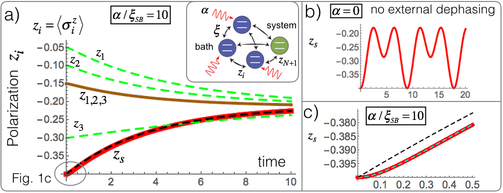
Figure 1: (a) The red curve shows the (exact) polarization of the system $z_{s}$ as a function of time, while the brown solid line stands for the polarizations of the bath spins when starting from a uniform polarization state ($z_{1}=z_{2}=z_{3})$. The dashed-black line shows the Markovian approximation (6) with respect to the exact dynamics when the dephasing is stronger than the system-bath coupling $\alpha/\xi_{SB}=10$. In the ’all to all’ coupling completely different initial bath preparations with the same initial total polarization (green dashed lines) lead to the exact same system dynamics (red curve). Thus, in this ideal-like bath the only important parameter of the bath is the total energy. (b) When the external dephasing is off ($\alpha=0$) equilibrium is not reached due to quantum recurrences. (c) For very short evolution time the Markovian approximation (dashed-black (6)) fails but our non-Markovian correction (dashed-cyan (3)) accurately describes the evolution.

Weak vs. strong coupling in dephased baths

When the coupling of the system to the bath $\xi_{SB}$ is much weaker than the coupling between different spins in the bath $\xi_{ij}^{B}$ ($i,j<N+1)$ the dynamics greatly simplifies. In the presence of dephasing and $\xi_{ij}^{B}\gg\xi_{SB}$, the bath spins equilibrate among themselves before the system changes significantly. Thus, (3) is valid also for configuration such as NN with weak system-bath coupling (see Appendix). In the Appendix we write an equation similar to (3) for the NN configuration when $\xi_{ij}^{B}\gg\xi_{SB}$ does not hold.

System-bath correlation in small dephased baths

Next we study the creation of system-bath correlation during Markovian and non-Markovian dynamics of the system. When the system is weakly coupled to a large bath, the correlation between the system and the bath can be made negligible and be ignored. This is not the case for small baths. In the following we discuss both the NN and the ATA configurations. As an illustrative example in the NN setup we use three spins for the bath with $\alpha=6$, $\xi_{B}=1$ and $\xi_{SB}=1/20$. For the ATA setup we also use three spins for the bath and $\alpha=6,\xi=1/(20\sqrt{3})$. As a result, the Markovian decay time for both configurations is the same, and is equal to $\tau_{MARK}=\alpha/(2\xi_{SB}^{2})=1200$. The top curves in Fig. 2a show that the system polarization in the NN configuration (red curve), and the polarization in the ATA configuration (dashed blue) have practically the same evolution. The tiny difference arises from the fact that the bath spins (lower curves show $z_{1},z_{2},z_{3}$) do not yet perfectly equlibriate among themselves. Correction to Markovian dynamics are observed only on a scale of $1/\alpha=1/6$. These correlations are classical since off-diagonal elements are negligible in the presence of strong dephasing. We study the correlation by looking at the standard statistical correlation $\text{corr}(i,j)=\text{cov}(z_{i},z_{j})/[\text{var}(z_{i})\text{var}(z_{i})]$. The dashed-blue curve in Fig. 2b shows the correlation between any of the bath spins and the system in the ATA configuration. A more interesting dynamics takes place in the NN setup. Remarkably, even though the bath spins in the NN case have almost exactly the same polarizations (Fig. 2a), their correlation with the system differ significantly at $1/\alpha\leq t\ll\tau_{MARK}$ as shown by the red curves in Fig. 2b (see the inset for a magnification). This highly interesting correlation equilibration at a rate much slower than the polarization equilibration warrants further study.

Another interesting feature in the correlation evolution is the asymptotic value obtained for $t\gg\tau_{MARK}$. While the transient correlation evolution depends on the coupling strength and on the coupling configuration, the asymptotic value $\mathit{\text{corr}{}_{\infty}}$ depends only on the initial conditions. This can be understood from the fact that $\sum_{i\neq j}^{N+1}\left\langle\sigma_{i}^{z}\sigma_{j}^{z}\right\rangle$ is a conserved quantity in for choice of $\xi_{ij}$. Using this conserved quantity together with energy conservation, and the fact that the final equilibrium state is completely uniform, we obtain the asymptotic correlation $\mathit{\text{corr}{}_{\infty}}=[\frac{1}{(N-1)N}\sum_{i\neq j}^{N+1}\left\langle\sigma_{i}^{z}\sigma_{j}^{z}\right\rangle_{t=0}-z_{\infty}^{2}]/(1/4-z_{\infty}^{2}).$ When the spins are initially uncorrelated and the bath starts in a uniform polarization this expression simplifies to

$$\mathit{\text{corr}{}_{\infty}}=-\frac{(z_{T}-z_{s}(0))^{2}}{(M+1)^{2}}/(1/4-z_{\infty}^{2})$$ (7)

Note that regardless of the configuration, at $t\to\infty$ the system is equally correlated to all bath spins. $\text{corr}{}_{\infty}$ is negative for any $M$, $z_{T}$, and $z_{s}(0)$. Moreover, since $z_{\infty}\to z_{T}$ for large $N$, we conclude from (7) that the asymptotic correlation scales like $1/(M+1)^{2}$ when $z_{T}$ and $z_{s}(0)$ are kept fixed. Hence, $\mathit{\text{corr}{}_{\infty}}\to 0$ for large bath. We conclude that the unavoidable asymptotic system-bath correlation is another unique feature that appears in small dephased bath, even when the dynamics is fully Markovian. In small non-dephased baths the correlation will also be strong but the correlation will oscillate without reaching a steady state.

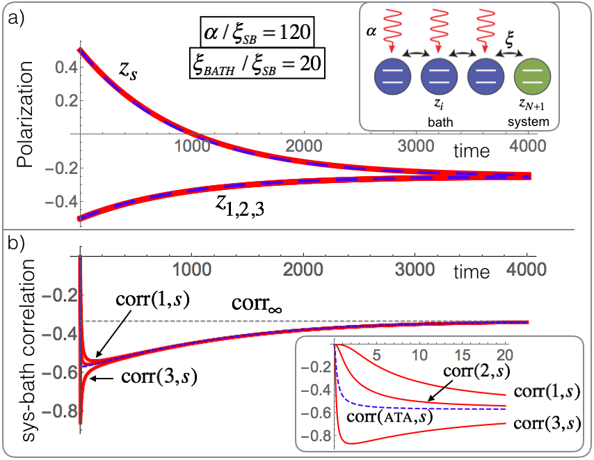
Figure 2: In our scheme is strong system-bath correlation can form even when the system follows Markovian dynamics. (a) In the weak coupling limit in the NN configuration (see inset), the polarization dynamics (red curves) is the same as that of the ATA configuration (blue dashed curves) when the ATA configuration is set to have the same decay time $\alpha/(2\xi_{SB})^{2}$. Yet, the system-bath correlation (b) in the NN setup (red) is non-uniform even when the bath polarization is highly uniform (see inset). The the ATA correlation is shown in the dashed-blue curve. While the peak correlation depends on the setup parameters, the unavoidable asymptotic correlation $\text{corr}{}_{\infty}$ (7) is fixed by the initial conditions and cannot be mitigated by weak system-bath coupling.

Experimental realization in ion traps

Quantum simulation of spin Hamiltonians has been demonstrated using trapped atomic ions Friedenauer et al. (2008); Kim et al. (2010); Jurcevic et al. (2014). An effective spin 1/2 system (pseudo-spin) is realized using two internal levels of the ion which can be separated by radio-frequency, microwave or optical transitions. By using spin dependent forces that couple internal and translational degrees of freedom, it is possible to generate various interactions between the ions. In the Appendix we discuss NN and ATA realization in ion traps, and find that it should be possible to implement a dephased bath scheme with the current experimental capabilities.

Experimental realization superconducting circuits

dephased baths can be also readily implemented in superconducting circuits. By coupling transmon-type superconducting qubits Koch et al. (2007) to a common far detuned resonator the NN and the ATA configurations can be implemented. In the Appendix we provide estimates and mention previously implemented building blocks. The superconducting architecture also allows to experimentally explore possible extensions of this work, including studies of system-bath correlations, continuously driven open system Gasparinetti et al. (2013), etc.

Conclusion

We have introduced a paradigm for the implementation of Markovian heat sources with the smallest possible heat capacity. Despite the Markovian dynamics we have identified features in our setup that are unique to small heat sources: 1) An enhanced decay rate with respect to the decoherence rate 2) A significant, and unavoidable system-bath correlation that cannot be eliminated by reducing the system-bath coupling. In addition, we find a correlation equilibration time that is much larger than the bath polarization equilibration time. Finally, our theoretical approach also provides an accurate reduced description for the non-Markovian dynamics at short evolution times.

We have studied realizations in ion traps and in superconducting qubits where the “all to all” coupling can be implemented. In our dephased bath setup the ATA coupling has the remarkable property that the system is sensitive only to the total energy in the bath. This makes the ATA bath an ideal bath: the internal dynamics inside the bath does not affect the reduced dynamics of the system. This greatly simplifies the preparation stage of the bath: any preparation with the same energy will do.

Potentially, these baths can serve as a practical element in experiments. Furthermore, this setup motivates new questions about open quantum systems. For example, the study of accumulated system-bath correlation is a complicated topic that is greatly simplified in the dephased bath setup proposed here. In addition, it is intriguing to study dephasing in quantum system with larger Hilbert space (qudits) and to include system-bath particle exchange.

Appendix

Derivation of the equation of motion

The system-bath setup dynamics is modeled by a Lindblad equation

$$d_{t}\rho=-i[H,\rho]+\sum 2A_{k}\rho A_{k}^{\dagger}-A_{k}^{\dagger}A_{k}\rho-\rho A_{k}^{\dagger}A_{k},$$ (8)

where $A_{k}$ describes the external dephasing environment, and $H$ is given by Eq. (1) in the main text. By moving to the interaction picture $H_{0}$ is eliminated and $V$ remains unaffected Since we $[H_{0},V]=0$. To obtain a dephasing rate $\alpha$ for spin $i$ we set $A_{k}=\sqrt{\alpha}\sigma_{i}^{z}$ . Note that for two-spins $A_{1}$ (or $A_{2}$) will also lead to dephasing at a rate $\alpha$ of coherences that involve both spins for example element $\rho_{2,3}$ in the joint density matrix.

We start the derivation of the equation of motion by writing the equation for the time derivative of polarization of the system spin $z_{s}=\left\langle\sigma_{s}^{z}\right\rangle$

$$d_{t}z_{s} =\text{tr}\{-i\sigma_{s}^{z}[V,\rho]$$

$$+\sigma_{s}^{z}\sum 2A_{k}\rho A_{k}^{\dagger}-A_{k}^{\dagger}A_{k}\rho-\rho A_{k}^{\dagger}A_{k}\}.$$ (9)

Since $[A_{k},\sigma^{z}]=0$

$$d_{t}z_{s} =\text{tr}[-i\sigma_{s}^{z}(V\rho-\rho V)]=-i\text{tr}([\sigma_{s}^{z},V]\rho).$$

In contrast to other methods for obtaining reduced dynamics that are based on integration (see the microscopic derivation H.-P. Breuer and F. Petruccione (2002)), we start with differentiation

$$d_{t}^{2}z_{s} =\text{tr}\{-i\sigma_{s}^{z}[H,d_{t}\rho]$$

$$+\sigma_{s}^{z}\sum 2A_{k}d_{t}\rho A_{k}^{\dagger}-A_{k}^{\dagger}A_{k}d_{t}\rho-d_{t}\rho A_{k}^{\dagger}A_{k}\}$$ (10)

$$=\text{tr}\{-\sigma_{s}^{z}[V,[V,\rho]]\}$$

$$-\alpha\text{tr}\{i\sigma_{s}^{z}[V,(\sum_{k}2\sigma_{k}^{z}\rho\sigma_{k}^{z}-\frac{1}{2}\rho)\}.$$ (11)

Let us first study the first term (quadratic in $V$)

$$\text{tr}\{\sigma_{s}^{z}[V,[V,\rho]]\}= \text{tr}\{\rho[[\sigma_{s}^{z},V],V]\}$$

$$= \text{tr}\{\rho[[\sigma_{s}^{z},\sum_{k}^{N}V_{s,k}],\sum_{j=1}^{N+1}V_{k,j}]\}$$

$$= \sum_{k}^{N}\text{tr}\{\rho[[\sigma_{s}^{z},V_{s,k}],V_{s,k}]\}$$

$$+ tr\{\rho[[\sigma_{s}^{z},\sum_{k}^{N}V_{s,k}],\sum_{j=1}^{N}V_{k,j}]\}$$

$$= \sum_{k=1}^{N}2(z_{s}-z_{k})\xi_{sk}^{2}$$

$$+ 2\sum_{k,j=1}^{N}\xi_{sk}\xi_{sj}(\left\langle\sigma_{k}^{-}\sigma_{j}^{z}\sigma_{s}^{+}\right\rangle+c.c.)$$

$$+ 2\sum_{k,j=1}^{N}\xi_{sk}\xi_{sj}(\left\langle\sigma_{k}^{-}\sigma_{s}^{z}\sigma_{j}^{+}\right\rangle+c.c.).$$ (12)

Next we study the second term in (11) (Linear in $\alpha$)

$$\alpha\text{tr}\{i\sigma_{s}^{z}[V,(\sum_{k}2\sigma_{k}^{z}\rho\sigma_{k}^{z}-\frac{1}{2}\rho)\} =\alpha i\text{tr}\sum_{k}\rho\sigma_{k}^{z}[\sigma_{s}^{z},V]\sigma_{k}^{z}$$

$$=-i\alpha\text{tr}\sum_{k}\rho[\sigma_{s}^{z},V]$$

$$=\alpha d_{t}\left\langle z\right\rangle,$$ (13)

where we have used the relation $\sigma^{z}\sigma^{\pm}\sigma^{z}=-\frac{1}{4}\sigma^{\pm}$ . Finally we get

$$\frac{d^{2}}{dt^{2}}z_{s}=-2\sum\xi_{sk}^{2}(z_{s}-z_{k})-\alpha\frac{dz_{s}}{dt}+O(\left\langle\sigma^{-}\sigma^{z}\sigma^{+}\right\rangle).$$ (14)

where $\left\langle\sigma^{-}\sigma^{z}\sigma^{+}\right\rangle$ denotes the last two terms in (12). The terms represented by $\left\langle\sigma^{-}\sigma^{z}\sigma^{+}\right\rangle$ correspond to off-diagonal elements in total density matrix. In particular, these elements connect different spins (i.e., it is not just the coherence of the system spin) as such, these elements are strongly suppressed by the external dephasing, and can safely be neglected.

Note that in general $z_{k}=z_{k}(t)$ so this equation is not closed and cannot be solved without prior knowledge of $z_{k}(t)$. There are scenarios, though, in which this equation is closed, and can be solved. One is the all to all coupling, and the other is weak coupling. In the all to all coupling $\xi_{sk}=\xi$ so we can write

$$\frac{d^{2}}{dt^{2}}z_{s} =-2\xi^{2}Nz_{s}+2\xi^{2}\sum_{k}(z_{k})-\alpha\frac{dz_{s}}{dt}$$

$$=-2\xi^{2}Nz_{s}+2\xi^{2}(z_{tot}-z_{s})-\alpha\frac{dz_{s}}{dt}$$

$$=-2\xi^{2}(N+1)z_{s}-2\xi^{2}z_{tot}-\alpha\frac{dz_{s}}{dt}$$

$$=-2\xi^{2}(N+1)(z_{s}-\frac{z_{tot}}{N+1})-\alpha\frac{dz_{s}}{dt}.$$ (15)

Finally, we get

$$\frac{d^{2}}{dt^{2}}z_{s}=-2N\xi^{2}\frac{N+1}{N}(z_{s}-z_{\infty})-\alpha\frac{dz_{s}}{dt}$$ (16)

In the weak coupling limit $z_{1}=z_{2}=...=z_{N}\neq z_{s}$. As before the average polarization is a conserved quantity so we can write $z_{k}(t)=[(N+1)z_{\infty}-z_{s}(t)]/N$ and get

$$\frac{d^{2}}{dt^{2}}z_{s} =-2(\sum\xi_{sk}^{2})\frac{N+1}{N}(z_{s}-z_{\infty})-\alpha\frac{dz_{s}}{dt},$$ (17)

which has the same form as (16) just with different coupling strength.

An extended dephasing time in small baths $T_{2}\leq 2\frac{N+1}{N}T_{1}$

Consider a completely positive Markovian map (8) with $H=0$ for simplicity. $z_{0}$ is the asymptotic polarization of the map. The polarization of the system $\left\langle\sigma^{z}\right\rangle$ can be changed by setting the Lindblad operators to $A_{1}=\sqrt{g_{+}}\sigma^{+},\>A_{2}=\sqrt{g_{-}}\sigma^{-}$. We start by studying a map with time-independent asymptotic polarization $\frac{dz_{0}}{dt}=0$ and get from (8)

$$\frac{d}{dt}z =-2(g_{+}+g_{-})(z-z_{0}).$$ (18)

$$z_{0}=\frac{1}{2}\frac{g_{+}-g_{-}}{g_{+}+g_{-}},$$ (19)

The coherence dynamics is obtained by looking on $\left\langle x\right\rangle=tr[\rho\sigma^{x}]$ that satisfies

$$\frac{d}{dt}x=-(g_{+}+g_{-})x.$$ (20)

The solutions (18) and (20) are

$$\frac{z(t)-z_{0}}{z(0)-z_{0}} =\exp[-2(g_{+}+g_{-})t]\triangleq e^{-\gamma_{z}t},$$ (21)

$$\frac{x(t)}{x(0)} =\exp[-(g_{+}+g_{-})t]\triangleq e^{-\gamma_{x}t}.$$ (22)

Using these solution we compare the polarization decay rate $\gamma_{z}$ and the coherence decay rate $\gamma_{x}$ and get

$$\frac{\gamma_{z}}{\gamma_{x}}=2.$$ (23)

Note that we have used the fact that $\frac{dz_{0}}{dt}=0$. Adding elements like $A_{3}=\sigma_{z}$ will increase $\frac{d}{dt}x$ but will not affect $\frac{d}{dt}z$ and therefore we get the standard result for completely positive Markovian dynamics Gorini and Kossakowski (1976); Chang and Skinner (1993)

$$\gamma_{z}\leq 2\gamma_{x}.$$ (24)

In our case the map is time-dependent . The rate $(g_{+}+g_{-})$ is fixed by the physical couplings, but $z_{0}$ (related to $g_{+}-g_{-}$) changes in time since the bath is finite. Using the polarization conservation $z_{0}(t)=\frac{(N+1)z_{\infty}-z_{s}}{N}$ we find

$$\frac{d}{dt}z_{s}=-2(g_{+}+g_{-})\frac{N+1}{N}(z_{s}-z_{\infty}),$$ (25)

and therefore

$$\gamma_{z}\leq 2\frac{N+1}{N}\gamma_{x}.$$ (26)

Thus, the polarization decay rate can be faster than the minimal value of $2\gamma_{x}$ allowed for Markovian maps with a time-independent $z_{0}$. Note that this dressing effect does not happen for $x$ since the dephasing constantly eliminates any bath coherence that may come from interacting with the system.

Experimental realization in ion traps

To synthesize significant pseudo-spin interaction Hamiltonians between the ions in the trap, spin-dependent forces are used. These forces can be realized, for example, by optical fields acting on optically separated pseudo-spin levels, or by Raman transitions on microwave-separated pseudo spin levels. Spin-dependent forces induce spin-dependent motion of ions in the trap, leading to the acquisition of spin-dependent phases, and thus to an effective spin-spin interaction. To mimic the effect of spin-interaction Hamiltonians and not only their time-evolution operator at specific times, quantum simulations are conducted using spin-dependent forces that are tuned far off-resonance from one, or more, of the crystal normal-modes of motion. Thus, excited motion can be adiabatically eliminated and the interaction between the spins becomes direct. Here, spin-spin interaction can be thought of as mediated by the exchange of virtual crystal-phonons. A transverse field in the $z$ direction can be introduced by detuning the pseudo-spin transition from the Raman or optical interaction. The dephasing of bath spins is straightforward to implement using individual-addressing of bath ions with off-resonant laser beams that will shift them from resonance in a quasi-random time sequence.

The implementation of different $\xi_{i,j}$, depends on the normal modes of motion that are used. This can be done by spectrally tuning the lasers or microwave fields that induce spin-dependent forces. ATA coupling can be achieved in ion-traps by tuning spin-dependent forces close to the center-of-mass mode of an ion crystal in which all ions oscillate in-phase, and with equal amplitude, along the trap axis Friedenauer et al. (2008). Thus the ATA configuration discussed above can be readily implemented. The use of spin-dependent forces that act on radial normal modes in ions traps was shown to lead to relative flexibility in determining $\xi_{i,j}$. In particular it was shown that when radial modes are spectrally closely-spaced, the range of spin-spin interactions can be scanned between $0\leq\delta\leq 3$ where $\xi_{i,j}\propto 1/|i-j|^{\delta}$ and $i$ and $j$ are the locations of the ions in the chain, by tuning the spin-dependent force frequency close to or far from the radial modes respectively Kim et al. (2011). While the synthesis of arbitrary $\xi_{i,j}$ was shown to be possible Korenblit et al. (2012) it will be very difficult to experimentally implement. The implementation of the NN configuration will therefore be challenging using trapped-ion systems, although it could be fairly well approximated using $\xi_{i,j}\propto 1/|i-j|^{3}$ where the next-to-nearest neighbor interaction is suppressed by a factor of eight.

Experimental realization in Superconducting circuits

For definiteness, we focus on superconducting qubits of the transmon type Koch et al. (2007). These qubits have good coherence properties, can be individually addressed, made to interact, and read out with high fidelity. Hence, they are currently being considered as building blocks for quantum computation Devoret and Schoelkopf (2013). In particular, they were recently used to study thermalization of an isolated quantum system Neill et al. (2016). The interaction between any pair $(i,j)$ of qubits can be realized using a common resonator as quantum bus Blais et al. (2004, 2007) and takes the form $H_{I}=g_{i}g_{j}\left(\Delta_{i}^{-1}+\Delta_{j}^{-1}\right)\left(\sigma_{+,j}\sigma_{-,i}+\sigma_{+,i}\sigma_{-,j}\right)$, where $g_{i}$ are the qubit-resonator couplings, $\Delta_{i}=\omega_{i}-\omega_{r}$ is the detuning between the qubit frequency $\omega_{i}$ and the resonator frequency $\omega_{r}$, and the expression is valid in the strong-detuning limit, $\Delta_{i}/g_{i}\gg 1$. This interaction realizes a two-qubit $\sqrt{i{\rm SWAP}}$ gate, mediated by virtual interaction with the resonator. The interaction is effectively switched off by “parking” the qubits in a largely detuned configuration, and switched on by nonadiabatically tuning the qubits in resonance with each other and closer in frequency to the resonator. (The qubit frequencies can be adjusted on a fast time scale by changing the local magnetic field at each qubit’s site.) The NN scheme can be realized by arranging the qubits in a one-dimensional chain and coupling each neighboring pair by an individual bus resonator Salathé et al. (2015). The ATA scheme can be realized by coupling all qubits to a common resonator, as recently demonstrated for an ensemble of ten qubits in Ref. Song et al. (2017). Based on these experiments, we estimate that a tunable interaction strength $\xi/2\pi=5\text{MHz}$ can be reached in both configurations. Single-qubit dephasing of arbitrary strength can be engineered by injecting classical noise into the system, causing fluctuations in the local magnetic field and hence in the qubit frequency. Due to spurious coupling to uncontrolled degrees of freedom the superconducting qubits have an intrinsic thermalization time $T_{1}$. We require that the thermalization rate of the system via the dephased bath be much larger than its intrinsic relaxation rate, $\xi^{2}/\alpha\gg 1/T_{1}$, so that the composite system can be considered as isolated during the thermalization time. At the same time, observing the full crossover between unitary dynamics and Zeno freezing requires $\xi/\alpha\ll 1$. Even assuming a conservative $T_{1}\approx 10\leavevmode\nobreak\ \mu{\rm s}$, ratios as low as $\xi/\alpha\approx 1/20$ can be attained with intrinsic relaxation still playing a negligible role.

References

- Seifert (2012) U. Seifert, Reports on Progress in Physics 75, 126001 (2012).
- Harris and Schütz (2007) R. Harris and G. Schütz, Journal of Statistical Mechanics: Theory and Experiment 2007, P07020 (2007).
- Goold et al. (2016) J. Goold, M. Huber, A. Riera, L. del Rio, and P. Skrzypczyk, Journal of Physics A: Mathematical and Theoretical 49, 143001 (2016).
- Vinjanampathy and Anders (2016) S. Vinjanampathy and J. Anders, Contemporary Physics 57, 545 (2016).
- Millen and Xuereb (2016) J. Millen and A. Xuereb, New Journal of Physics 18, 011002 (2016).
- Gour et al. (2015) G. Gour, M. P. Müller, V. Narasimhachar, R. W. Spekkens, and N. Y. Halpern, Physics Reports 583, 1 (2015).
- Lostaglio et al. (2015) M. Lostaglio, D. Jennings, and T. Rudolph, Nature communications 6, 6383 (2015).
- Uzdin (2016a) R. Uzdin, arXiv preprint arXiv:1609.05742 (2016a).
- Mitchison et al. (2015) M. T. Mitchison, M. P. Woods, J. Prior, and M. Huber, New Journal of Physics 17, 115013 (2015).
- Uzdin et al. (2015) R. Uzdin, A. Levy, and R. Kosloff, Phys. Rev. X 5, 031044 (2015).
- Uzdin (2016b) R. Uzdin, Phys. Rev. Applied 6, 024004 (2016b).
- Niedenzu et al. (2016) W. Niedenzu, D. Gelbwaser-Klimovsky, A. G. Kofman, and G. Kurizki, New Journal of Physics 18, 083012 (2016).
- H.-P. Breuer and F. Petruccione (2002) H.-P. Breuer and F. Petruccione, Open quantum systems (Oxford university press, 2002).
- Scovil and Schulz-DuBois (1959) H. E. D. Scovil and E. O. Schulz-DuBois, Phys. Rev. Lett. 2, 262 (1959).
- Eitan Geva and Ronnie Kosloff (1994) Eitan Geva and Ronnie Kosloff, Phys. Rev. E 49, 3903 (1994).
- Kofman and Kurizki (2000) A. G. Kofman and G. Kurizki, Nature 405, 546 (2000).
- Erez et al. (2008) N. Erez, G. Gordon, M. Nest, and G. Kurizki, Nature 452, 724 (2008).
- Rao and Kurizki (2011) D. B. Rao and G. Kurizki, Physical Review A 83, 032105 (2011).
- Chenu et al. (2017) A. Chenu, M. Beau, J. Cao, and A. Del Campo, Physical Review Letters 118, 140403 (2017).
- Gorini and Kossakowski (1976) V. Gorini and A. Kossakowski, J. Math. Phys. 17, 1298 (1976).
- Chang and Skinner (1993) T.-M. Chang and J. Skinner, Physica A: Statistical Mechanics and its Applications 193, 483 (1993).
- Friedenauer et al. (2008) A. Friedenauer, H. Schmitz, J. T. Glueckert, D. Porras, and T. Schätz, Nature Physics 4, 757 (2008).
- Kim et al. (2010) K. Kim, M.-S. Chang, S. Korenblit, R. Islam, E. Edwards, J. Freericks, G.-D. Lin, L.-M. Duan, and C. Monroe, Nature 465, 590 (2010).
- Jurcevic et al. (2014) P. Jurcevic, B. P. Lanyon, P. Hauke, C. Hempel, P. Zoller, R. Blatt, and C. F. Roos, Nature 511, 202 (2014).
- Koch et al. (2007) J. Koch, T. M. Yu, J. Gambetta, A. A. Houck, D. I. Schuster, J. Majer, A. Blais, M. H. Devoret, S. M. Girvin, and R. J. Schoelkopf, Phys. Rev. A 76, 042319 (2007).
- Gasparinetti et al. (2013) S. Gasparinetti, P. Solinas, S. Pugnetti, R. Fazio, and J. P. Pekola, Phys. Rev. Lett. 110, 150403 (2013).
- Kim et al. (2011) K. Kim, S. Korenblit, R. Islam, E. Edwards, M. Chang, C. Noh, H. Carmichael, G. Lin, L. Duan, C. J. Wang, et al., New Journal of Physics 13, 105003 (2011).
- Korenblit et al. (2012) S. Korenblit, D. Kafri, W. C. Campbell, R. Islam, E. E. Edwards, Z.-X. Gong, G.-D. Lin, L. Duan, J. Kim, K. Kim, et al., New Journal of Physics 14, 095024 (2012).
- Devoret and Schoelkopf (2013) M. Devoret and R. J. Schoelkopf, Science 339, 1169 (2013).
- Neill et al. (2016) C. Neill, P. Roushan, M. Fang, Y. Chen, M. Kolodrubetz, Z. Chen, A. Megrant, R. Barends, B. Campbell, B. Chiaro, A. Dunsworth, E. Jeffrey, J. Kelly, J. Mutus, P. J. J. O[rsquor]Malley, C. Quintana, D. Sank, A. Vainsencher, J. Wenner, T. C. White, A. Polkovnikov, and J. M. Martinis, Nat Phys 12, 1037 (2016).
- Blais et al. (2004) A. Blais, R.-S. Huang, A. Wallraff, S. M. Girvin, and R. J. Schoelkopf, Phys. Rev. A 69, 062320 (2004).
- Blais et al. (2007) A. Blais, J. Gambetta, A. Wallraff, D. I. Schuster, S. M. Girvin, M. H. Devoret, and R. J. Schoelkopf, Phys. Rev. A 75, 032329 (2007).
- Salathé et al. (2015) Y. Salathé, M. Mondal, M. Oppliger, J. Heinsoo, P. Kurpiers, A. Potočnik, A. Mezzacapo, U. Las Heras, L. Lamata, E. Solano, S. Filipp, and A. Wallraff, Phys. Rev. X 5, 021027 (2015).
- Song et al. (2017) C. Song, K. Xu, W. Liu, C. Yang, S. Zheng, H. Deng, Q. Xie, K. Huang, Q. Guo, L. Zhang, P. Zhang, D. Xu, D. Zheng, X. Zhu, H. Wang, Y. . Chen, C. . Lu, S. Han, and J. . Pan, arXiv:1703.10302 (2017).