Higher lying resonances in low-energy electron scattering with carbon monoxide

Abstract

$\mathbf{R}$-matrix calculations on electron collisions with CO are reported whose aim is to identify any higher-lying resonances above the well-reported and lowest ${}^{2}\Pi$ resonance at about 1.6 eV. Extensive tests with respect to basis sets, target models and scattering models are performed. The final results are reported for the larger cc-pVTZ basis set using a 50 state close-coupling (CC) calculation. The Breit-Wigner eigenphase sum and the time-delay methods are used to detect and fit any resonances. Both these methods find a very narrow ${}^{2}\Sigma^{+}$ symmetry Feshbach-type resonance very close to the target excitation threshold of the b ${}^{3}\Sigma^{+}$ state which lies at 12.9 eV in the calculations. This resonance is seen in the CC calculation using cc-pVTZ basis set while a CC calculation using the cc-pVDZ basis set does not produce this feature. The electronic structure of CO^- is analysed in the asymptotic region; 45 molecular states are found to correlate with states dissociating to an anion and an atom. Electronic structure calculations are used to study the behaviour of these states at large internuclear separation. Quantitative results for the total, elastic and electronic excitation cross sections are also presented. The significance of these results for models of the observed dissociative electron attachment of CO in the 10 eV region is discussed.

1 Introduction

Low-energy electron collisions with the carbon monoxide molecules display a broad ${}^{2}\Pi$ symmetry shape resonance at about 1.6 eV. This resonance has been well-characterised experimentally HM83 ; Allan89 ; gmg96 ; pbv06 ; allan10 and is the subject of a number of theoretical studies gmg96 ; sbn84 ; Morgan91 ; wmz13 ; jt527 . This resonance provides the main mechanism for electron impact vibrational excitation jt527 ; jt621 but lies too low in energy to lead to dissociative electron attachment (DEA) unless the CO target is also vibrationally excited jt621 .

There are a number of theoretical studies which consider collision energies of above 5 eV; these have generally focused on electron impact electronic excitation cross sections wh90 ; jt140 ; lmf96 ; lib02 ; gmm05 ; rtj10 . However, experimentally it has long been known that CO can undergo dissociative electron attachment (DEA) with two peaks at about 10.2 and 10.9 eV rb65 ; ss70 ; cr71 ; ss71 ; 75cth ; hcs77 ; nn15 and the main product of this is C+O^-, although C^-+O has also been observed ss70 . The precise physics of the states contributing to the DEA process has recently proved somewhat controversial nn15 ; twx13 ; nn15b ; tl15 ; wxl15 .

DEA is assumed to occur via resonances. Several works, both experimental and theoretical, exist on the resonance features around 10 eV. In fact, a ${}^{2}\Sigma+$ resonance at 10.04 eV was identified and known to contribute to DEA as early as 1973 Schulz73 . There are two R-matrix calculations which showed resonance features above 20 eV. In one, Salvini et al sbn84 suggested that CO has a ${}^{2}\Sigma^{+}$ shape resonance at about 20 eV; there is no other evidence for this state. Similarly, in another calculation, Morgan and Tennyson jt140 found a rather broad, widths greater than 1 eV, resonance for each of the doublet symmetries they considered. Their resonance curves all looked rather similar. It is at least possible that these features are a consequence of employing a target wavefunction which extended outside the R-matrix sphere; this was found to produce artificial resonances in subsequent calculations on water mor98 ; jt281 . Weatherford and Huo wh90 performed a two-state calculation using Hartree-Fock wavefunctions and also found 4 resonances in the 10 - 20 eV region.

The available cross section data for electron collisions with carbon monoxide have recently been collected and reviewed by Itikawa Itikawa15 . These data are important for understanding discharges, including the CO laser wc75 ; GC84 ; kb15 , other CO plasmas 14ccd and a variety of astronomical applications lv94 ; cb09 ; cab11 as CO is thought to be the second most common molecule in the Universe after H₂.

Given the significance of DEA of CO, it is important to try and build a viable theoretical model for this process. As a first step it is necessary to identify possible resonances through which the DEA may occur. An aim of this paper is to identify resonances in the 10 – 12 eV region. In this context we note that an 11.5 eV ${}^{2}\Sigma_{g}^{+}$ resonance has been identified in the isoelectronic N₂ from both experiment and theory haf09 . However this theoretical work used bound state methodology to characterise the resonance, a procedure that is not without dangers jt241 . Similarly, Pearson and Lefebvre-Brion performed stabilization calculations on the CO^- systems and identified a single, narrow ${}^{2}\Sigma^{+}$ symmetry resonance at 10.2 eV pl76 .

2 Theory

The general theory of the $\mathbf{R}$-matrix method and its specific implementations in the UK molecular $\mathbf{R}$-matrix  codes, to study various aspects in electron and positron collision with molecules, has been described in detail in a recent review by one of us jt474 . Therefore, we limit ourself to the essential parts that are necessary for the subsequent discussions.

The $\mathbf{R}$-matrix method involves separation of space around the electron+target collision system depending upon the kind of interaction between the target molecule and the scattering electron. This separation is usually done using an imaginary sphere, called the $\mathbf{R}$-matrix  sphere, centred at the centre-of-mass of the molecule. The radius of the sphere is chosen such that it contains the entire wave function of the $N$-electron target states. Inside the sphere, called the inner region, the collision complex is described by fully taking care of the exchange and correlation effects among all the $N+1$ electrons. The inner region wave function, $\psi_{k}^{N+1}$, is expressed as a close-coupling (CC) expansion:

$$\begin{split}\psi_{k}^{N+1}&=\mathcal{A}\sum_{ij}a_{ijk}\Phi_{i}^{N}(\textbf{x}_{1}...\textbf{x}_{N})u_{ij}(\textbf{x}_{N+1})\\ &\quad+\sum_{i}b_{ik}\chi_{i}^{N+1}(\textbf{x}_{1}...\textbf{x}_{N+1})\>,\end{split}$$ (1)

where, in the first term, $\Phi_{i}^{N}$ is the wave function of the $i$-th target state, $u_{ij}$ are the continuum orbitals to represent the scattering electron and $\mathcal{A}$ is the anti-symmetrization operator. In the second term, the $\chi_{i}^{N+1}$ are the so-called $L^{2}$ configurations, which are constructed by occupation of all $N+1$ electrons to the target molecular orbitals (MOs).

Different scattering models can be constructed by choosing different types of expansions for the target wave function ($\Phi_{i}^{N}$) and the corresponding $L^{2}$ configurations in Eq. (1). Generally three different models are used, namely, the static exchange (SE), SE plus polarization (SEP) and the close-coupling (CC) models. The SE and SEP models are among the simplest approximations to the scattering problem and only use the ground state of the target, represented by a Hartree-Fock (HF) self consistent field (SCF) wave function. Using the SE, one can describe only the shape resonances and compute the elastic cross section. While SEP can represent Feshbach resonances, these are often not well represented without inclusion of their parent electronic state. CC models are more sophisticated and involve inclusion of several target states which themselves can be represented by different methods. Usually, the complete active space (CAS) configuration interaction (CI) method is chosen for representation of the target states jt189 . The CC model can describe Feshbach resonances and also compute electron impact electronic excitation cross sections. Even more sophisticated is the molecular $\mathbf{R}$-matrix  with pseudo-states (RMPS) method jt341 ; jt354 . However this method rapidly leads to huge calculations jt444 and, given the number of excited electronic states of the target that need to be explicitly considered here (see below), a full RMPS study was deemed to be impractical. A recent attempt to treat several target electronic states of the simpler, 10-electron methane system shows how large such calculations rapidly become jt585 .

At the boundary of the $\mathbf{R}$-matrix  sphere, the $\mathbf{R}$-matrix  is built, for different scattering energies, from the boundary amplitude of the inner region wave functions and the $\mathbf{R}$-matrix  poles. Then, the $\mathbf{R}$-matrix  is propagated to large distances in order to match to the analytical asymptotic functions. The matching yields the $\mathbf{K}$-matrix as a function of scattering energy. The $\mathbf{K}$-matrix is a key quantity and other scattering observables can be obtained from it.

Finding and characterizing resonances is a major aspect of any electron-molecule scattering study. In this study our goal is to find any higher lying resonances above the lowest and well-known ${}^{2}\Pi$ shape resonance. In order to do this we use two quantities, the eigenphase sum and time-delay, to find and fit the resonances.

The eigenphase sum fitting method is the standard method to detect resonances in many studies. When the eigenphase sum is plotted against the scattering energy resonances appear as sudden jumps by $\pi$ over a small energy region haz79 . Once located, the resonance parameters can be found by fitting the eigenphase sum $\delta(E)$ to the Breit-Wigner form

$$\delta(E)=\delta_{0}(E)+\tan^{-1}\frac{\Gamma}{2(E^{r}-E)}\>,$$ (2)

where $\delta_{0}(E)$ is the background eigenphase, $E^{r}$ is the resonance position and $\Gamma$ is the width. However, this method struggles to fit closely spaced and overlapping resonances or ones near to a threshold. The fitting of eigenphase sum to the Breit-Wigner form is automatically done by the module RESON jt31 in the UKRmol codes jt518 .

The above problems can be overcome in the time-delay method and it is, therefore, the method of choice for detecting resonances in electron collision with ionic targets, where there are large number of closely spaced resonances. The time-delay method was first proposed by Smith smi60 and was first implemented in the UKRmol codes by Stibbe and Tennyson jt188 through the module TIMEDEL jt227 . Recently, it has been updated by Little et al. jt650 and used to study electron collision with $N_{2}^{+}$ jt574 . If the largest (first) eigenvalue of the time-delay matrix (i.e., the longest time-delay) is plotted against scattering energy then the resonances appear as Lorentzians. The TIMEDEL module automatically fits up to the highest three eigenvalues as a function of energy ($q(E)$) to a Lorentzian of the form:

$$q(E)=\frac{\Gamma}{(E-E^{r})^{2}+(\Gamma/2)^{2}}+bg(E)\>,$$ (3)

where $bg(E)$ is the background.

3 Calculation & Results

In this study we perform fixed-nuclei $\mathbf{R}$-matrix calculations for CO at the equilibrium bond distance, $R_{eq}=2.1323$ a₀. The molecular orbitals necessary for the target and scattering calculations are obtained from MOLPRO molpro06 . The scattering calculations are performed using the UK molecular $\mathbf{R}$-matrix  codes jt225 ; jt238 . These codes have been recently modernized and upgraded to treat many different processes in electron and positron scattering with molecules jt518 , and are called the UKRmol codes. Since neither the polyatomic implementation of UKRmol used here nor MOLPRO can treat CO in its natural symmetry of $C_{{\infty}v}$ we use the Abelian point group of $C_{2v}$. Since identification of the target and resonant scattering states in the $C_{2v}$ symmetry group to the $C_{{\infty}v}$ is clear, we report these states using their natural symmetry group. For the molecular orbitals (MOs) we use the $C_{2v}$ point group designations.

We have performed extensive tests with respect to different target and scattering models. Our strategy had been to do these tests with the smaller cc-pVDZ basis set in order to find a good and yet computationally manageable model for the scattering calculations. Then, we performed the final calculations using the bigger cc-pVTZ basis set with the chosen model.

3.1 Target calculations

As described above, different scattering models involve use of different types of target wave functions in the expansion in Eq. (1). In the SE and SEP model only the target ground state represented at the SCF level is used. The SCF ground state energy and dipole moment of CO is found to be $-112.74928$ E_h and $-0.23$ Debye, respectively, for the cc-pVDZ basis set. The HF electronic ground state configuration of CO is given as $[(1a_{1}-5a_{1})^{10},(1b_{1})^{2},(1b_{2})^{2}]$ in $C_{2v}$ symmetry or as $[(1\sigma-5\sigma)^{10},(1\pi)^{4}]$ in $C_{{\infty}v}$ symmetry.

For the use in scattering calculations with the CC model, we performed systematic CASSCF studies on the target using various active spaces for the cc-pVDZ basis set. These active spaces are defined in Table 1. The smallest and commonly used active space is the full valence CAS (FVCAS), where all 10 valence electrons are distributed among all 8 valence MOs, keeping the 4 core electrons frozen. We call this as CAS(10,8) and the electron configuration is given as: $(1a_{1}-2a_{1})^{4}\,(3a_{1}-6a_{1},1b_{1}-2b_{1},1b_{2}-2b_{2})^{10}$. The largest CASSCF calculation we performed is the CAS(10,15) which, in addition to the valence MOs, also included the lower $\sigma$ and $\pi$ molecular orbitals, formed from the 3s and 3p atomic orbitals of C and O, in the active space. This calculation took more than 30 hours for a sequential MOLPRO run on a 64-bit machine. In order to do our final scattering calculations we choose, however, the computationally more modest CAS(10,10) model. This is because the scattering calculation with any larger active space would become unmanageably large with the larger cc-pVTZ basis set despite the use of a specially-designed algorithm for Hamiltonian generation jt180 .

A selected set of results from these CASSCF calculations for the cc-pVDZ basis set is given in Table 2. These calculations are performed for 40 target states, which includes the lowest 5 states from each space-spin symmetry. Therefore, the MOs used in the CC scattering calculations are the state-averaged CASSCF (SA-CASSCF) orbitals having equal weights from each state. The table compares the ground state energy (in $E_{h}$), vertical excitation energies (in eV) to the lowest 9 states and ground state dipole moments (in Debye) among different CASSCF models. As can be seen the relative vertical excitation energies are fairly close to each other in these CASSCF models. The table also includes the results from CAS(10,10) calculation using the cc-pVTZ basis set. For the cc-pVTZ basis set we made a 50 states SA-CASSCF calculation, where in addition to the above said 40 target states we included 5 more states from each of the ${}^{1}A_{1}$ and ${}^{3}A_{1}$ symmetries. This was done in order to include a greater number of $\Sigma^{+}$ target states in the CC scattering calculation, as the $A_{1}$ state in $C_{2v}$ symmetry contains both $\Sigma^{+}$ and $\Delta$ states. Having done this, we can see in the Table 2 that the second ${}^{3}\Sigma^{+}$ target state becomes the ninth lowest excited state. Available experimental (adiabatic) excitation energies are also included in the table for comparison. These values are derived by Nielsen et al.nie80 from the spectroscopic constants of Huber and Herzberg hub79 . Their spectroscopic assignments are given in the parenthesis. As can be seen the experimental values are quite consistent with our vertical excitation energies from the cc-pVTZ basis set.

3.2 Asymptotic states

As discussed below there are significant number of states of the CO^- system which lie below the dissociation limit of CO into C(³P) and O(³P). Note that here and elsewhere we neglect spin-orbit effects which lead to the splitting of these and other atomic terms values.

To help understand the high energy resonance structure in CO^- we performed an analysis of these states. Table 3 shows the number and symmetry of the states which dissociate to the four bound asymptotes, C(³P) + O^-(²P), C^-(⁴S) + O(³P), C(¹D) + O^-(²P) and C^-(²D) + O(³P). Based on the electron affinities for O Blondel95 and C, Feld77 these dissociation products are bound by 1.461, 1.262, 0.197 and 0.033 eV, respectively.

As detailed in Table 3, there are 45 separate molecular curves which lead asymptotically to states of CO^- and asymptotically lie below the C + O ground state. In principle any of these curves could be involved in dissociative attachment and have an associated resonance signature at short internuclear separations, $R$. To understand this situation better it was decided to perform a series of electronic structure calculations to characterise these states. In doing this we concentrate on the large $R$ region where the electronic states are bound with respect to the CO ground state so as to avoid spurious effects which can arise from performing bound electronic structure calculation in the continuum jt241 .

Calculations were performed using MOLPRO, which provides a range of quantum chemical methods normally used for computing bound electronic states. Such calculations can be used to describe resonant anionic states in the asymptotic region when it crosses and lies below that of the neutral ground state. In the resonant region it will require scattering methods (like the R-matrix theory), or possibly stabilization procedures, to correctly describe the potential energy curves (PECs).

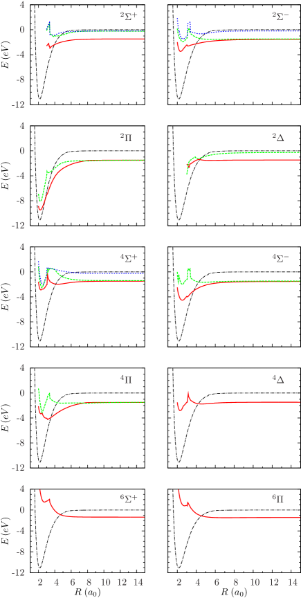
Figure 1: CO^- potential energy curves grouped by symmetry. The dashed black curve is the X ${}^{1}\Sigma^{+}$ CO ground state. The number of curves are chosen using the numbers expected for each symmetry, see Table 3.

In computing the PECs we use the aug-cc-pVTZ basis set for C and O. The diffuse functions in the augmented basis set are necessary to describe the anionic states. The PECs are computed at the multi-reference configuration interaction (MRCI) level of theory with Davidson correction. This method is generally refered to as the MRCI+Q method. The Davidson correction is an extrapolation method to the full-CI limit. The necessary molecular orbitals are calculated from a state-averaged CASSCF(11,10) calculation at the specified bond length. The active space for the chosen CASSCF calculation is defined as: $(1a_{1}-2a_{1})^{4}\,(3a_{1}-6a_{1},1b_{1}-3b_{1},1b_{2}-3b_{2})^{11}$. The role of choice of CAS in the calculation of excited electronic states has recently come under scrutiny jt623 ; jt632 but was not explored here. Figure 1 summarises our results. The energies reported are from MRCI+Q calculations and plotted with respect to the dissociation energy of the neutral ground state CO molecule and converted to eV.

Figure 1 suggests that the sextet states (${}^{6}\Sigma^{+}$ and ${}^{6}\Pi$) as well as the ${}^{4}\Delta$ states are all repulsive at short $R$. For the other symmetries the calculations at least suggest that there are states which could result in resonance features in the 10 - 15 eV region. The only other exception to this is the ${}^{2}\Pi$ symmetry which, of course, shows the clear signature of the well-known ${}^{2}\Pi$ shape resonance but the next curve appears to become a quasi-continuum state at short bond lengths as its shape simply mirrors that of the CO ground state curve. Our calculations show that the lowest ${}^{2}\Pi$ shape resonance correlates asymptotically with C(³P) + O^-(²P) and that the lowest ${}^{2}\Sigma^{+}$ curves goes asymptotically to C^-(⁴S) + O(³P).

3.3 Scattering calculations

All the reported scattering calculations use an $\mathbf{R}$-matrix sphere of radius $a=10\ a_{0}$. The continuum orbitals, which represent the scattering electron, are expanded in a basis of Gaussian-type functions centred on the centre-of-mass of the target jt286 . The continuum orbitals with partial waves $\ell\leq 4$ are included in these calculation. These orbitals are Schmidt orthogonalized to the target MOs and then all MOs are symmetrically orthogonalized to each other. As noted above, in the SE model the target MOs are SCF orbitals while in CC model these are SA-CASSCF orbitals. Only those MOs that have eigenvalues, from the symmetrical orthogonalization, larger than a deletion threshold of $10^{-7}$ are retained in the calculation.

The results of the scattering calculations using various models and the cc-pVDZ basis set are shown in the Table 4. The SE model, unsurprisingly, finds only the ${}^{2}\Pi$ shape resonance whose position and width are too large in comparison to the larger models. All our CC calculations using the cc-pVDZ basis set also find only one resonance, that is the lowest ${}^{2}\Pi$ shape resonance. Even the 40 states CC calculation using a larger active space of CAS(10,11) find only this resonance.We note that the inner region calculation for A₁ symmetry with the larger CAS(10,11) took 5.5 days to finish in comparison to using the CAS(10,10) which took only 5 hours.

In this study we do not report the results of SEP model. Our previous experience jt459 with SEP calculations showed that the resonance parameters do not converge as the number of virtual MOs included increases. This is because of the deteriorating balance between the target and scattering calculation. The scattering calculation improves upon addition of more number of virtual MOs while the target energy remains fixed in its ground state SCF representation. However, in an older SEP calculation on carbon monoxide, Morgan Morgan91 reported convergence of the lowest ${}^{2}\Pi$ resonance position and width with respect to increase in number of virtual MOs. That calculation, however, was only for the energy region below the first electronic excitation threshold. In SEP there is also another problem due to the occurrence of the non-physical pseudo-resonances jt474 . This problem arises because of the fact that while this model includes polarization effect it does not, however, include the excited target states in the expansion in Eq. (1).

Our ‘best’ results are from the CC calculation which included 50 target states represented by CAS(10,10) using the cc-pVTZ basis set. Since the $\mathbf{R}$-matrix method is based on the variational principle, a lower value for resonance position also means we have better approximation to the exact scattering wave function. In this model the ${}^{2}\Pi$ resonance position is found to be at 1.73 eV, which is lower in comparison with all the models tested using the cc-pVDZ basis set. We also find a new resonance in this model for the ${}^{2}A_{1}$ symmetry. Since it does not appear in the calculation for ${}^{2}A_{2}$ symmetry, we can assign it the ${}^{2}\Sigma^{+}$ symmetry in $C_{\infty{v}}$ point group.

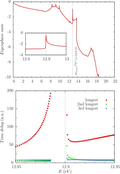
Figure 2: ${}^{2}A_{1}$ resonance: the upper panel shows the eigenphase sum as a function of scattering energy from our best model (see text for details). The inset shows the narrow Feshbach resonance at 12.9 eV, lying extremely close to the $2\;^{3}\Sigma^{+}$ target state. The lower panel shows the time-delay plot in the resonance region.

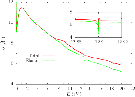
Figure 3: Total and elastic cross section for ${}^{2}A_{1}$ symmetry. The inset shows the effect of the Feshbach resonance to the cross sections.

The ${}^{2}\Sigma^{+}$ resonance is clearly seen in the eigenphase sum plot for the ${}^{2}A_{1}$ symmetry in Fig. 2. The position of this resonance is found to be 12.899988 eV with a width of 0.000525 eV as fitted by RESON. The resonance position is extremely close to the b  ${}^{3}\Sigma^{+}$ threshold at 12.900787 eV. In the region of a threshold, the time-delay becomes infinite because the scattering electron associated with the newly opening channel moves with zero kinetic energy. This can be seen in the plot of time-delay in Fig. 2 where the time-delay diverges at 12.9 eV. Therefore, we could not get the fitted resonance parameters from the TIMEDEL module. Since this resonance has a very narrow width of 0.52 meV and appears extremely close to the $2\,^{3}\Sigma^{+}$ target state at 12.9 eV, we therefore characterize it as a core-excited Feshbach resonance with the $2\,^{3}\Sigma^{+}$ target state as its parent, to which it is bound only by about 0.0008 eV. The effect of the resonance on the cross sections can be seen Fig. 3.

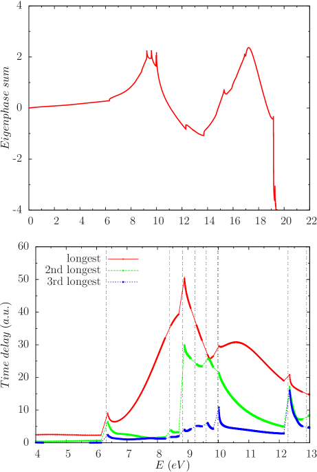
Figure 4: Eigenphase sum plot (upper) and time-delay plot (lower) for ${}^{2}A_{2}$ symmetry. The broken vertical lines indicate the electronic excitation thresholds.

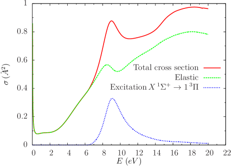
Figure 5: Total, elastic and the dominant electron impact excitation cross section of CO in the ${}^{2}A_{2}$ symmetry.

We present the eigenphase sum and time-delay for ${}^{2}A_{2}$ symmetry from our best model in Fig. 4. The plot for total, elastic and the dominant electron impact excitation cross section of CO is given in Fig. 5. The cross section plot shows a broad peak at 9 eV. However, the eigenphase sum and time-delay plots do not show any feature associated with a resonance. Neither the eigenphase sum and time-delay fitting modules (RESON and TIMEDEL) find or fit any resonance for this symmetry. We, however, suspect that the peak structure at 9 eV will become a resonance at larger bond distances. We have started doing $\mathbf{R}$-matrix calculations as a function of bond distance with a view to investigating this and other aspects.

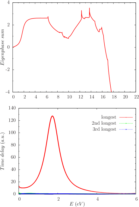
Figure 6: Eigenphase sum plot (upper) and time-delay plot (lower) for ${}^{2}B_{1}$ symmetry.

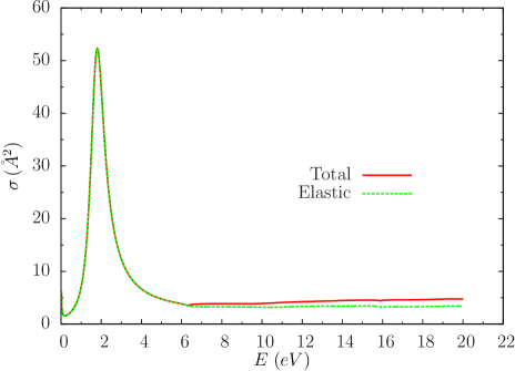
Figure 7: Total and elastic cross section for ${}^{2}B_{1}+^{2}B_{2}$ (${}^{2}\Pi$) symmetry.

The eigenphase sum and time-delay plots, from our best model, for the ${}^{2}B_{1}$ symmetry are presented in Fig. 6; these are identical to those obtained for the degenerate ${}^{2}B_{2}$ symmetry calculation. The resonance feature around 2 eV is fitted by both RESON and TIMEDEL to the same values of position of 1.73 eV and width of 0.84 eV. The elastic and total cross section due the ${}^{2}\Pi$ (${}^{2}B_{1}+^{2}B_{1}$) symmetry is given in Fig. 7

4 Discussion

The DEA experiments suggest that there are two ${}^{2}\Sigma^{+}$ resonances between 10 eV and 11 eV rb65 ; ss70 ; cr71 ; ss71 ; 75cth ; hcs77 ; nn15 . Our calculations detected only a single ${}^{2}\Sigma^{+}$ resonance at 12.9 eV. It is therefore worth discussing this difference.

There has long been experimental evidence that excited electronic states of small molecules in the 10 to 15 eV region often support a complicated set of Feshbach resonances Schulz73 . So far, theory has only made a modest contribution to modelling and interpreting these resonances. It is useful to consider the case of electron – H₂ collisions where resonances in the 10 to 15 eV have been well-studied. $\mathbf{R}$-matrix  calculations on this system jt90 ; jt101 ; jt215 mapped out resonances as a function of internuclear separation to give resonance curves. However, these calculations also found many “features” where the eigenphase sums showed structures in form of resonance-like jumps, but that these jumps were significantly smaller than one would expect from a fully-formed resonance jt101 . Some of these features became resonances as the internuclear separation was changed. Furthermore, even for H₂, where with a two-electron target it is was possible to perform full CI calculations, it was necessary to shift the resonance positions to fully reproduce the observed behaviour jt208 . This was done by identifying the parent associated with each Feshbach resonance and then mapping this to highly accurate ab initio curves which are, of course, available for H₂. Even here there is a complication, as studies have shown, that Feshbach resonances could often not be associated with a single parent state jt199 . These H${}_{2}^{-}$ resonance curves have recently been used for theoretical studies of DEA and vibrational excitation of H₂ via these high-lying resonances jt507 ; jt567 . We note that there was a concerted attempt to map out such higher-lying Feshbach resonance in water. Here systematic studies of H₂O^- resonances hzm04 ; jt359 ; drw05 ; drw07 gave useful comparisons with experiment but obtaining complete agreement with the observations remains more difficult has11 ; 13sha . A similar methodology has been applied to CO₂ sar11 and methane dsa15 in the 10 eV region.

For CO, the 10.04 eV ${}^{2}\Sigma^{+}$ resonance and its effect on the DEA was reported by Schulz Schulz73 . More recently, experimental DEA studies were undertaken by Nag and Nandy nn15 and Tian et. al. twx13 . These studies proved somewhat controversial regarding the nature of the resonances involved. Whereas Nag and Nandy indicated the involvement of ${}^{2}\Sigma^{+}$ and ${}^{2}\Pi$ resonances in the DEA around 10-12 eV, Tian et al proposed that the DEA in the range 10-12 eV occurs through a coherent superposition of ${}^{2}\Pi$, ${}^{2}\Delta$ and ${}^{2}\Phi$ states at lower end of the energy range while at higher energies above 12.1 eV the resonant states in the superposition are changed to ${}^{2}\Sigma$, ${}^{2}\Delta$ and ${}^{2}\Phi$.

Such higher lying resonances were reported in experimental studies of integral cross sections in vibrationally elastic transitions in CO jz96a ; jz96 . These studies suggest that there were several ${}^{2}\Sigma^{+}$ Feshbach resonances in the region above 10.04 eV associated with the b ${}^{3}\Sigma^{+}$ and higher lying parent states.

Returning to the present results we find a ${}^{2}\Sigma^{+}$ symmetry resonance 0.0008 eV below the second ${}^{3}\Sigma^{+}$ target state. This state, which is known from experiment and labelled the b ${}^{3}\Sigma^{+}$ state, has been the subject of $\mathbf{R}$-matrix  studies which used electron collisions with CO⁺ to characterize high-lying excited states of CO jt189 ; jt373 . These studies suggest that the vertical excitation energy of the b ${}^{3}\Sigma^{+}$ state is in the region of 10.2 to 10.4 eV, in good agreement with the observed result which places this at 10.4 eV ts72 . It would therefore seem likely the the ${}^{2}\Sigma^{+}$ Feshbach resonance we detect lies somewhere in this region. Once nuclear motion effects due to zero point energy, which is about 0.27 eV for CO, and other effects are taken into account it would seem likely that this resonance is responsible for the 10.2 eV DEA feature. This would be in agreement with the stabilization calculations of Pearson and Lefebvre-Brion pl76 who also only identified a single resonance in the 10 eV region, and also in line with Nag and Nandy’s nn15 assertion that a ${}^{2}\Sigma^{+}$ resonance is involved in DEA in this region.

A recent, detailed ab initio study by Vázquez et al val09 of electronically excited states of CO demonstrate just how complicated the curves are as function of internuclear separation in this region. Unfortunately Vázquez et al did not consider states of ${}^{3}\Sigma^{+}$ symmetry so cannot be used to inform our study.

So if we have successfully identified the lower of the two resonance features, what about the resonance responsible for DEA at 10.9 eV? There would appear to be two possibilities here. We see a number of features which could not be fully characterized as resonances in our calculations. It is possible that as the bond length increases one of these becomes a proper resonance which correlate with one of the many CO^- asymptotic states we identify and hence can lead to DEA. However, it is more likely that this resonance is associated with a target state which lies even higher than the b ${}^{3}\Sigma^{+}$ state. Table 2 only considers the 9 lowest electronically excited states of CO. In fact our calculation uses 50 states of CO but the higher states give increasing unrealistic representations of the physical target states; indeed many of them lie above the CO ionization threshold. It would appear that to make progress it would be necessary to design a model with an increased number of actual target states (as opposed to pseudo-states) explicitly included in the model.

5 Conclusion

We have performed an initial $\mathbf{R}$-matrix  study to try and identify the resonance states responsible for dissociative electron attachment (DEA) in the electron – CO system. We identify a very narrow ${}^{2}\Sigma^{+}$ Feshbach resonance which would appear to be the feature which causes DEA at about 10.2 eV. In future work we will study this resonance as function of internuclear separation, which should allow a full model of the DEA process to be built. The narrowness of this resonance will make the nuclear motion part of this model rather straightforward since non-adiabatic effects can almost certainly be neglected.

Our calculations failed to identify further higher-lying resonances. It is likely that such resonance are associated with parent target states that is not well-represented in our model. The higher-lying electronic states in CO are increasingly Rydberg-like jt189 ; val09 and therefore difficult to represent using standard target models. Furthermore, including such Rydberg states in a scattering calculation remains very challenging jt585 and will probably require further work on the methodology we use for such scattering calculations, for example the routine use of extended $\mathbf{R}$-matrix  spheres. Such work is currently being undertaken as part of the development of the B-spline-based UKRMol+ codes Masin ; initial results on the much simpler electron – BeH collision system have demonstrated the methods ability to deal with very diffuse target states and include a comprehensive treatment of target electron correlation Darby .

Table 1: The active space configurations used in the target CASSCF calculations. The molecular orbitals are labelled using $C_{2v}$ point group.

CASSCF models	Configurations
CAS(10,8)	$(1a_{1}-2a_{1})^{4}\,(3a_{1}-6a_{1},1b_{1}-2b_{1},1b_{2}-2b_{2})^{10}$
CAS(10,9)	$(1a_{1}-2a_{1})^{4}\,(3a_{1}-7a_{1},1b_{1}-2b_{1},1b_{2}-2b_{2})^{10}$
CAS(10,10)	$(1a_{1}-2a_{1})^{4}\,(3a_{1}-6a_{1},1b_{1}-3b_{1},1b_{2}-3b_{2})^{10}$
CAS(10,11)	$(1a_{1}-2a_{1})^{4}\,(3a_{1}-7a_{1},1b_{1}-3b_{1},1b_{2}-3b_{2})^{10}$
CAS(10,12)	$(1a_{1}-2a_{1})^{4}\,(3a_{1}-8a_{1},1b_{1}-3b_{1},1b_{2}-3b_{2})^{10}$
CAS(10,13)	$(1a_{1}-2a_{1})^{4}\,(3a_{1}-9a_{1},1b_{1}-3b_{1},1b_{2}-3b_{2})^{10}$
CAS(10,14)	$(1a_{1}-2a_{1})^{4}\,(3a_{1}-8a_{1},1b_{1}-4b_{1},1b_{2}-4b_{2})^{10}$
CAS(10,15)	$(1a_{1}-2a_{1})^{4}\,(3a_{1}-9a_{1},1b_{1}-4b_{1},1b_{2}-4b_{2})^{10}$

Table 2: The ground state energy (in E_h), the lowest 9 vertical excitation energies (in eV) and ground state dipole moments ($\mu$ in D) of CO calculated using varying active spaces with cc-pVDZ and using CAS(10,10) with cc-pVTZ basis sets. See text for details. Experimental values derived by Nielsen et al. nie80 from the spectroscopic constants of Huber and Herzberg hub79 are given for comparison.

State	cc-pVDZ								cc-pVTZ	Expt
	CAS(10,8)	CAS(10,9)	CAS(10,10)	CAS(10,11)	CAS(10,12)	CAS(10,13)	CAS(10,14)	CAS(10,15)	CAS(10,10)
$X\,^{1}\Sigma^{+}$	-112.85537	-112.86388	-112.89473	-112.92428	-112.92723	-112.93840	-112.95161	-112.95146	-112.85655
$1\,^{3}\Pi$	6.49	6.52	6.40	6.39	6.38	6.56	6.38	6.41	6.31	6.32 ($a\,^{3}\Pi$)
$1\,^{3}\Sigma^{+}$	8.69	8.69	8.79	8.83	8.80	8.78	8.80	8.72	8.39	8.51 ($a^{\prime}\,{}^{3}\Sigma^{+}$)
$1\,^{1}\Pi$	9.12	9.12	9.19	9.22	9.16	9.33	9.15	9.02	8.83	8.51 ($A\,^{1}\Pi$)
$1\,^{3}\Delta$	9.62	9.64	9.76	9.81	9.80	9.80	9.80	9.74	9.23	9.36 ($d\,^{3}\Delta$)
$1\,^{3}\Sigma^{-}$	10.00	10.02	10.15	10.20	10.18	10.19	10.16	10.12	9.60	9.88 ($e\,^{3}\Sigma^{-}$)
$1\,^{1}\Sigma^{-}$	10.37	10.42	10.54	10.59	10.59	10.60	10.58	10.54	9.97	9.88 ($I\,^{1}\Sigma^{-}$)
$1\,^{1}\Delta$	10.41	10.46	10.57	10.62	10.61	10.64	10.59	10.57	10.00	10.23 ($D\,^{1}\Delta$)
$2\,^{3}\Pi$	12.84	12.91	12.65	12.89	12.89	12.88	12.78	12.75	12.29
$2\,^{1}\Pi$	14.36	14.40	14.24	14.45	14.41	14.48	14.30	14.24
$2\,^{3}\Sigma^{+}$									12.90
$\mu$	0.514	0.452	0.234	0.071	0.045	0.158	0.043	0.240	0.291	0.122

Table 3: Molecular curves correlating with the bound asymptotic states of CO^-; given are both the number of molecular states correlating with each dissociation product, $N$, and their symmetries. 2 ${}^{2}\Sigma^{-}$ means two states of ${}^{2}\Sigma^{-}$ symmetry and so forth. Binding energies, $E_{b}$, are given relative to C(³P) + O(³P).

Product	$E_{b}$ / eV	$N$	Symmetries
C(3P) + O-(2P)	1.461	12	${}^{2}\Sigma^{+}$, 2 ${}^{2}\Sigma^{-}$, 2 ${}^{2}\Pi$, ${}^{2}\Delta$, ${}^{4}\Sigma^{+}$, 2 ${}^{4}\Sigma^{-}$, 2 ${}^{4}\Pi$, ${}^{4}\Delta$
C-(4S) + O(3P)	1.262	6	${}^{2}\Sigma^{+}$, ${}^{2}\Pi$, ${}^{4}\Sigma^{+}$, ${}^{4}\Pi$, ${}^{6}\Sigma^{+}$, ${}^{6}\Pi$
C(1D) + O-(2P)	0.197	9	2 ${}^{2}\Sigma^{+}$, ${}^{2}\Sigma^{-}$, 3 ${}^{2}\Pi$, 2 ${}^{2}\Delta$, ${}^{2}\Phi$
C-(2D) + O(3P)	0.033	18	2 ${}^{2}\Sigma^{+}$,${}^{2}\Sigma^{+}$, 3 ${}^{2}\Pi$, 2 ${}^{2}\Delta$, ${}^{2}\Phi$, 2 ${}^{4}\Sigma^{+}$, ${}^{4}\Sigma^{-}$, 3 ${}^{4}\Pi$, 2 ${}^{4}\Delta$, ${}^{4}\Phi$

Table 4: Positions (and widths) of the detected ${}^{2}\Pi$ and ${}^{2}\Sigma^{+}$ resonances computed using different scattering models. The label CAS(10,8)/cc40 represents a close-coupling calculation with 40 target states represented by CAS(10,8) model. None of our calculations using cc-pVDZ basis set detected the ${}^{2}\Sigma^{+}$ resonance. All quantities are in eV.

Basis sets	Models	${}^{2}\Pi$ resonance	${}^{2}\Sigma^{+}$ resonance
cc-pVDZ	SCF/SE	3.50 (1.96)
	CAS(10,8)/cc40	2.01 (0.83)
	CAS(10,10)/cc40	2.12 (0.91)
	CAS(10,10)/cc50	1.95 (0.81)
	CAS(10,11)/cc40	2.20 (0.95)
cc-pVTZ	CAS(10,10)/cc50	1.73 (0.84)	12.899988 (0.000525)

References

- (1) G.N. Haddad, H.B. Milloy, Australian J. Phys. 36, 473 (1983)
- (2) M. Allan, J. Electron Spectrosc. Related Phenom. 48, 219 (1989)
- (3) J.C. Gibson, L.A. Morgan, R.J. Gulley, M.J. Brunger, C.T. Bundschu, S.J. Buckman, J. Phys. B: At. Mol. Opt. Phys. 29, 3197 (1996)
- (4) G.B. Poparić, D.S. Belić, M.D. Vicić, Phys. Rev. A 73, 062713 (2006)
- (5) M. Allan, Phys. Rev. A 81, 042706 (2010)
- (6) S. Salvini, P.G. Burke, C.J. Noble, J. Phys. B: At. Mol. Opt. Phys. 17, 2549 (1984)
- (7) L.A. Morgan, J. Phys. B: At. Mol. Opt. Phys. 24, 4649 (1991)
- (8) W. Yuan-Cheng, M. Jia, Z. Ya-Jun, Chinese Phys. B 22, 023402 (2013)
- (9) V. Laporta, C.M. Cassidy, J. Tennyson, R. Celiberto, Plasma Sources Sci. Technol. 21, 045005 (2012)
- (10) V. Laporta, R. Celiberto, J. Tennyson, Plasma Sources Sci. Technol. 25, 01LT04 (2016)
- (11) C.A. Weatherford, W.M. Huo, Phys. Rev. A 41, 186 (1990)
- (12) L.A. Morgan, J. Tennyson, J. Phys. B: At. Mol. Opt. Phys. 26, 2429 (1993)
- (13) M.T. Lee, A.M. Machado, M.M. Fujimoto, L.E. Machado, L.M. Brescansin, J. Phys. B: At. Mol. Opt. Phys. 29, 4285 (1996)
- (14) M.T. Lee, I. Iga, L.M. Brescansin, L.E. Machado, F.B.C. Machado, J. Molec. Struct. (THEOCHEM) 585, 181 (2002)
- (15) M. Gracas, R. Martins, A.M. Maniero, L.E. Machado, J.D.M. Vianna, Brazilian J. Phys 35, 945 (2005)
- (16) R. Riahi, P. Teulet, N. Jaidane, A. Gleizes, Eur. Phys. J. D 56, 67 (2010)
- (17) D. Rapp, D.D. Briglia, J. Chem. Phys. 43, 1480 (1965)
- (18) A. Stamatovic, G.J. Schulz, J. Chem. Phys. 53, 2663 (1970)
- (19) J. Comer, F.H. Read, J. Phys.B: At. Mol. Phys. 4, 1678 (1971)
- (20) L. Sanche, G.J. Schulz, Phys. Rev. Lett. 26, 943 (1971)
- (21) I. Cadex, M. Tronc, R.I. Hall, J. Phys. B: At. Mol. Opt. Phys. 8, L73 (1975)
- (22) R.I. Hall, I. Cadex, C. Schermann, M. Tronc, Phys. Rev. A 15, 599 (1977)
- (23) P. Nag, D. Nandi, Phys. Chem. Chem. Phys. 17, 7130 (2015)
- (24) S.X. Tian, B. Wu, L. Xia, Y.F. Wang, H.K. Li, X.J. Zeng, Y. Luo, J. Yang, Phys. Rev. A 88, 012708 (2013)
- (25) P. Nag, D. Nandi, Phys. Rev. A 91, 056701 (2015)
- (26) S.X. Tian, Y. Luo, Phys. Rev. A 91, 056702 (2015)
- (27) X.D. Wang, C.J. Xuan, Y. Luo, S.X. Tian, J. Chem. Phys. 143, 066101 (2015)
- (28) G.J. Schulz, Rev. Mod. Phys. 45, 423 (1973)
- (29) L.A. Morgan, J. Phys. B: At. Mol. Opt. Phys. 31, 5003 (1998)
- (30) J.D. Gorfinkiel, L.A. Morgan, J. Tennyson, J. Phys. B: At. Mol. Opt. Phys. 35, 543 (2002)
- (31) Y. Itikawa, J. Phys. Chem. Ref. Data 44, 013105 (2015)
- (32) T. Wang, Q. Cheng, Optics Laser Tech. 33, 475 (2001)
- (33) C. Gorse, M. Capitelli, Chem. Phys. 85, 177 (1984)
- (34) T. Kozak, A. Bogaerts, Plasma Sources Sci. Technol. 24, 015024 (2015)
- (35) M. Capitelli, G. Colonna, G. D’Ammando, V. Laporta, A. Laricchiuta, Chem. Phys. 438, 31 (2014)
- (36) W.H. Liu, G.A. Victor, Astrophys. J. 435, 909 (1994)
- (37) L. Campbell, M.J. Brunger, Geophys. Res. Lett. 36, L03101 (2009)
- (38) L. Campbell, M. Allan, M.J. Brunger, J. Geophys. Res. 116, A09321 (2011)
- (39) T.H. Hoffmann, M. Allan, K. Franz, M.W. Ruf, H. Hotop, G. Sauter, W. Meyer, J. Phys. B: At. Mol. Opt. Phys. 42, 215202 (2009)
- (40) D.T. Stibbe, J. Tennyson, Chem. Phys. Lett. 308, 532 (1999)
- (41) P.K. Pearson, H. Lefebvre-Brion, Phys. Rev. A 13, 2106 (1976)
- (42) J. Tennyson, Phys. Rep. 491, 29 (2010)
- (43) J. Tennyson, J. Phys. B: At. Mol. Opt. Phys. 29, 6185 (1996)
- (44) J.D. Gorfinkiel, J. Tennyson, J. Phys. B: At. Mol. Opt. Phys. 37, L343 (2004)
- (45) J.D. Gorfinkiel, J. Tennyson, J. Phys. B: At. Mol. Opt. Phys. 38, 1607 (2005)
- (46) G. Halmová, J.D. Gorfinkiel, J. Tennyson, J. Phys. B: At. Mol. Opt. Phys. 41, 155201 (2008)
- (47) W.J. Brigg, J. Tennyson, M. Plummer, J. Phys. B: At. Mol. Opt. Phys. 47, 185203 (2014)
- (48) A.U. Hazi, Phys. Rev. A 19, 920 (1979)
- (49) J. Tennyson, C.J. Noble, Comput. Phys. Commun. 33, 421 (1984)
- (50) J.M. Carr, P.G. Galiatsatos, J.D. Gorfinkiel, A.G. Harvey, M.A. Lysaght, D. Madden, Z. Masin, M. Plummer, J. Tennyson, Eur. Phys. J. D 66, 58 (2012)
- (51) F.T. Smith, Phys. Rev. 118, 349 (1960)
- (52) D.T. Stibbe, J. Tennyson, J. Phys. B: At. Mol. Opt. Phys. 29, 4267 (1996)
- (53) D.T. Stibbe, J. Tennyson, Comput. Phys. Commun. 114, 236 (1998)
- (54) D. Little, J. Tennyson, M. Plummer, A. Sunderland, Comput. Phys. Commun. (2016)
- (55) D.A. Little, J. Tennyson, J. Phys. B: At. Mol. Opt. Phys. 47, 105204 (2014)
- (56) H.J. Werner, P.J. Knowles, F.R. Manby, M. Schütz et al., Molpro, version 2006.1, a package of ab initio programs (2006), see ”http://www.molpro.net”
- (57) L.A. Morgan, J. Tennyson, C.J. Gillan, Comput. Phys. Commun. 114, 120 (1998)
- (58) J. Tennyson, L.A. Morgan, Phil. Trans. A 357, 1161 (1999)
- (59) J. Tennyson, J. Phys. B: At. Mol. Opt. Phys. 29, 1817 (1996)
- (60) E.S. Nielsen, P. Jørgensen, J. Oddershede, J. Chem. Phys. 73, 6238 (1980)
- (61) K.P. Huber, G. Herzberg, Constants of Diatomic Molecules (Van Nostrand Reinhold, New York, 1979)
- (62) C. Blondel, Phys. Scripta T58, 31 (1995)
- (63) D. Feldmann, Chem. Phys. Lett. 47, 338 (1977)
- (64) L.K. McKemmish, S.N. Yurchenko, J. Tennyson, Mol. Phys. in press (2016)
- (65) J. Tennyson, L. Lodi, L.K. McKemmish, S.N. Yurchenko, J. Phys. B: At. Mol. Opt. Phys. 49, 102001 (2016)
- (66) A. Faure, J.D. Gorfinkiel, L.A. Morgan, J. Tennyson, Comput. Phys. Commun. 144, 224 (2002)
- (67) A. Dora, L. Bryjko, T. van Mourik, J. Tennyson, J. Chem. Phys. 130, 164307 (2009)
- (68) S.E. Branchett, J. Tennyson, Phys. Rev. Lett. 64, 2889 (1990)
- (69) S.E. Branchett, J. Tennyson, L.A. Morgan, J. Phys. B: At. Mol. Opt. Phys. 23, 4625 (1990)
- (70) D.T. Stibbe, J. Tennyson, J. Phys. B: At. Mol. Opt. Phys. 31, 815 (1998)
- (71) D.T. Stibbe, J. Tennyson, Phys. Rev. Lett. 79, 4116 (1997)
- (72) D.T. Stibbe, J. Tennyson, J. Phys. B: At. Mol. Opt. Phys. 30, L301 (1997)
- (73) R. Celiberto, R.K. Janev, J.M. Wadehra, J. Tennyson, Chem. Phys. 398, 206 (2012)
- (74) R. Celiberto, R.K. Janev, V. Laporta, J. Tennyson, J.M. Wadehra, Phys. Rev. A 88, 062701 (2013)
- (75) D.J. Haxton, Z.Y. Zhang, C.W. McCurdy, T.N. Rescigno, Phys. Rev. A 69, 062713 (2004)
- (76) J.D. Gorfinkiel, A. Faure, S. Taioli, C. Piccarretta, G. Halmová, J. Tennyson, Eur. Phys. J. D 35, 231 (2005)
- (77) D.J. Haxton, T.N. Rescigno, C.W. McCurdy, Phys. Rev. A 72, 022705 (2005)
- (78) D.J. Haxton, C.W. McCurdy, T.N. Rescigno, Phys. Rev. A 75, 012710 (2007)
- (79) D.J. Haxton, H. Adaniya, D.S. Slaughter, B. Rudek, T. Osipov, T. Weber, T.N. Rescigno, C.W. McCurdy, A. Belkacem, Phys. Rev. A 84, 030701 (2011)
- (80) D.S. Slaughter, D.J. Haxton, H. Adaniya, T. Weber, T.N. Rescigno, C.W. McCurdy, A. Belkacem, Phys. Rev. A 87, 052711 (2013)
- (81) D.S. Slaughter, H. Adaniya, T.N. Rescigno, D.J. Haxton, A.E. Orel, C.W. McCurdy, A. Belkacem, J. Phys. B: At. Mol. Opt. Phys. 44, 205203 (2011)
- (82) N. Douguet, D.S. Slaughter, H. Adaniya, A. Belkacem, A.E. Orel, T.N. Rescigno, PCCP 17, 25621 (2015)
- (83) J. Zobel, U. Mayer, K. Jung, H. Ehrhardt, J. Phys. B: At. Mol. Opt. Phys. 29, 813 (1996)
- (84) J. Zobel, U. Mayer, K. Jung, H. Ehrhardt, H. Pritchard, C. Winstead, V. McKoy, J. Phys. B: At. Mol. Opt. Phys. 29, 839 (1996)
- (85) K. Chakrabarti, J. Tennyson, J. Phys. B: At. Mol. Opt. Phys. 39, 1485 (2006)
- (86) S.G. Tilford, J.D. Simmons, J. Phys. Chem. Ref. Data 1, 147 (1972)
- (87) G.J. Vázquez, J.M. Amero, H.P. Liebermann, H. Lefebvre-Brion, J. Phys. Chem. A 113, 13395 (2009)
- (88) Z. Masin, The UKRMol+ code (2016)
- (89) D. Darby-Lewis, Z. Masin, J. Tennyson, J. Phys. B: At. Mol. Opt. Phys. (to be submitted) (2016)