$KMR$ $k_{t}$-factorization procedure for the description of the $LHCb$ forward hadron-hadron $Z^{0}$ production at $\sqrt{s}=13\;TeV$

Abstract

Quit recently, two sets of new experimental data from the $LHCb$ and the $CMS$ collaborations have been published, concerning the production of the $Z^{0}$ vector boson in hadron-hadron collisions with the center-of-mass energy $E_{CM}=\sqrt{s}=13\;TeV$. On the other hand, in our recent work, we have conducted a set of $NLO$ calculations for the production of the electroweak gauge vector bosons, utilizing the unintegrated parton distribution functions ($UPDF$) in the frameworks of $Kimber$-$Martin$-$Ryskin$ ($KMR$) or $Martin$-$Ryskin$-$Watt$ ($MRW$) and the $k_{t}$-factorization formalism, concluding that the results of the $KMR$ scheme are arguably better in describing the existing experimental data, coming from $D0$, $CDF$, $CMS$ and $ATLAS$ collaborations. In the present work, we intend to follow the same $NLO$ formalism and calculate the rate of the production of the $Z^{0}$ vector boson, utilizing the $UPDF$ of $KMR$ within the dynamics of the recent data. It will be shown that our results are in good agreement with the new measurements of the $LHCb$ and the $CMS$ collaborations.

I Introduction

Traditionally, the production of the electroweak gauge vector bosons is considered as a benchmark for understanding the dynamics of the strong and the electroweak interactions in the Standard Model. It is also an important test to assess the validity of collider data. Many collaborations have reported numerous sets of measurements, probing different events in variant dynamical regions, in direct or indirect relation with such processes, to count a few see the references ATLAS-2012 ; ATLAS-2015 ; CMS-2011 ; ATLAS2016 ; CMS2015 ; LHCb-2012 ; LHCb-2013 ; LHCb-20151 ; LHCb-20152 ; LHCb-20153 . Among the most recent of these reports are the measurements of the production of $Z^{0}$ bosons at the $LHCb$ and $CMS$ collaborations, for proton-proton collisions at the $LHC$ for $\sqrt{s}=13TeV$, with different kinematical regions LHCb ; CMS . The $LHCb$ data are in the forward pseudorapidity region ($2<|\eta|<4.5$) while the $CMS$ measurements are in th central domain ($0<|\eta|<2.4$).

In our previous work NLO-W/Z , we have successfully utilized the transverse momentum dependent ($TMD$) unintegrated parton distribution functions ($UPDF$) of the $k_{t}$-factorization (the references KMR ; MRW ), namely the $Kimber$-$Martin$-$Ryskin$ ($KMR$) and $Martin$-$Ryskin$-$Watt$ ($MRW$) formalisms in the leading order ($LO$) and the next-to-leading order ($NLO$) to calculate the inclusive production of the $W^{\pm}$ and the $Z^{0}$ gauge vector bosons, in the proton-proton and the proton-antiproton inelastic collisions

$$P_{1}+P_{2}\to W^{\pm}/Z^{0}+X.$$ (1)

In order to increase the precision of the calculations, we have used a complete set of $2\to 3$ $NLO$ partonic sub-processes, i.e.

$$g^{*}(\textbf{k}_{1})+g^{*}(\textbf{k}_{2})\to V(\textbf{p})+q(\textbf{p}_{1})+\bar{q}^{\prime}(\textbf{p}_{2}),$$

$$g^{*}(\textbf{k}_{1})+q^{*}(\textbf{k}_{2})\to V(\textbf{p})+g(\textbf{p}_{1})+q^{\prime}(\textbf{p}_{2}),$$

$$q^{*}(\textbf{k}_{1})+\bar{q}^{{}^{\prime}*}(\textbf{k}_{2})\to V(\textbf{p})+g(\textbf{p}_{1})+g(\textbf{p}_{2}),$$ (2)

where $V$ represents the produced gauge vector boson. $\textbf{k}_{i}$ and $\textbf{p}_{i}$, $i=1,2$ are the 4-momenta of the incoming and the out-going partons. The results underwent comprehensive and rather lengthy comparisons and it was concluded that the calculations in the $KMR$ formalism are more successful in describing the existing experimental data (with the center-of-mass energies of $1.8$ and $8$ TeV) from the $D0$, $CDF$, $ATLAS$ and $CMS$ collaborations ATLAS2016 ; CMS2015 ; CDF96 ; CDF2000 ; D095 ; D098 ; D02000-1 ; D02000-2 ; D02001 . The success of the $KMR$ scheme (despite being of the $LO$ and suffering from some misalignment with its theory of origin, i.e. the $Dokshitzer$-$Gribov$-$Lipatov$-$Altarelli$-$Parisi$ ($DGLAP$) evolution equations, DGLAP1 ; DGLAP2 ; DGLAP3 ; DGLAP4 ) can be traced back to the particular physical constraints that rule its kinematics. To find extensive discussions regarding the structure and the applications of the $UPDF$ of $k_{t}$-factorization, the reader may refer to the references Modarres1 ; Modarres2 ; Modarres3 ; Modarres4 ; Modarres5 ; Modarres6 ; Modarres7 ; Modarres8 .

Meanwhile, arriving the new data from the $LHCb$ and $CMS$ collaborations, the references LHCb ; CMS , gives rise to the necessity of repeating our calculations at the $E_{CM}=13\;TeV$. This is in part due to the very interesting rapidity domain of the $LHCb$ measurements, since in the forward rapidity sector ($2<|\eta_{f}|<4.5$), one can effectively probe very small values of the Bjorken variable $x$ ($x$ being the fraction of the longitudinal momentum of the parent hadron, carried by the parton at the top of the partonic evolution ladder), where the gluonic distributions dominate and hence the transverse momentum dependency of the particles involving in the partonic sub-processes becomes important.

In the present work, we intend to calculate the transverse momentum and the rapidity distributions of the cross-section of production of the $Z^{0}$ boson using our $NLO$ level diagrams (from the reference NLO-W/Z ) and the $UPDF$ of the $KMR$ formalism. The $UPDF$ will be prepared using the $PDF$ of $MMHT2014-LO$, MMHT . In the following section, the reader will be presented with a brief introduction to the $NLO\otimes LO$ framework (i.e. $NLO$ $QCD$ matrix elements and $LO$ $UPDF$) that is utilized to perform these computations. The section II also includes the main description of the $KMR$ formalism in the $k_{t}$-factorization procedure. Finally, the section III is devoted to results, discussions and a thoroughgoing conclusion.

II $NLO\otimes LO$ framework, $KMR$ $UPDF$ and numerical analysis

Generally speaking, the total cross-section for an inelastic collision between two hadrons ($\sigma_{Hadron-Hadron}$) can be expressed as a sum over all possible partonic cross-sections in every possible momentum configuration:

$$\sigma_{Hadron-Hadron}= \sum_{a_{1},a_{2}=q,g}\int_{0}^{1}{dx_{1}\over x_{1}}\int_{0}^{1}{dx_{2}\over x_{2}}\int_{0}^{\infty}{dk^{2}_{1,t}\over k^{2}_{1,t}}\int_{0}^{\infty}{dk^{2}_{2,t}\over k^{2}_{2,t}}f_{a_{1}}(x_{1},k^{2}_{1,t},\mu_{1}^{2})f_{a_{2}}(x_{2},k^{2}_{2,t},\mu_{2}^{2})$$

$$\times \hat{\sigma}_{a_{1}a_{2}}(x_{1},k^{2}_{1,t},\mu_{1}^{2};x_{2},k^{2}_{2,t},\mu_{2}^{2}).$$ (3)

In the equation (3), $x_{i}$ and $k_{i,t}$ respectfully represent the longitudinal fraction and the transverse momentum of the parton $i$, while $f_{a_{i}}(x_{i},k^{2}_{i,t},\mu_{i}^{2})$ are the density functions of the $i^{th}$ parton. The second scale, $\mu_{i}$, are the ultra-violet cutoffs related to the virtuality of the exchanged particle (or particles) during the inelastic scattering. $\hat{\sigma}_{a_{1}a_{2}}$ are the partonic cross-sections of the given particles. For the production of the $Z^{0}$ boson, the equation (3) comes down to (for a detailed description see the reference NLO-W/Z )

$$\sigma(P+\bar{P}\rightarrow Z^{0}+X)=\sum_{a_{i},b_{i}=q,g}\int{dk_{a_{1},t}^{2}\over k_{a_{1},t}^{2}}\;{dk_{a_{2},t}^{2}\over k_{a_{2},t}^{2}}\;dp_{b_{1},t}^{2}\;dp_{b_{2},t}^{2}\;dy_{1}\;dy_{2}\;dy_{W/Z}\;\times$$

$${d\varphi_{a_{1}}\over 2\pi}\;{d\varphi_{a_{2}}\over 2\pi}\;{d\varphi_{b_{1}}\over 2\pi}\;{d\varphi_{b_{2}}\over 2\pi}\times$$

$${|\mathcal{M}(a_{1}+a_{2}\rightarrow Z^{0}+b_{1}+b_{2})|^{2}\over 256\pi^{3}(x_{1}x_{2}s)^{2}}\;f_{a_{1}}(x_{1},k_{a_{1},t}^{2},\mu^{2})\;f_{a_{2}}(x_{2},k_{a_{2},t}^{2},\mu^{2}).$$ (4)

$y_{i}$ are the rapidities of the produced particles (since $y_{i}\simeq\eta_{i}$ in the infinite momentum frame, i.e. $p_{i}^{2}\gg m_{i}^{2}$). $\varphi_{i}$ are the azimuthal angles of the incoming and the out-going partons at the partonic cross-sections. $|\mathcal{M}|^{2}$ represent the matrix elements of the partonic sub-processes in the given configurations. The reader can find a number of comprehensive discussions over the means and the methods of deriving analytical prescriptions of these quantities in the references NLO-W/Z ; LIP1 ; LIP2 ; LIP3 ; Deak1 . $s$ is the center of mass energy squared. Additionally, in the proton-proton center of mass frame, one can utilize the following definitions for the kinematic variables:

$$P_{1}={\sqrt{s}\over 2}(1,0,0,1),\;\;\;P_{2}={\sqrt{s}\over 2}(1,0,0,-1),$$

$$\textbf{k}_{i}=x_{i}\textbf{P}_{i}+\textbf{k}_{i,\perp},\;\;\;k_{i,\perp}^{2}=-k_{i,t}^{2},\;\;\;i=1,2\;.$$ (5)

Defining the transverse mass of the produced particles, $m_{i,t}=\sqrt{m^{2}_{i}+p_{i}^{2}}$, we can write,

$$x_{1} ={1\over\sqrt{s}}\left(m_{1,t}e^{+y_{1}}+m_{2,t}e^{+y_{2}}+m_{Z,t}e^{+y_{Z}}\right),$$

$$x_{2} ={1\over\sqrt{s}}\left(m_{1,t}e^{-y_{1}}+m_{2,t}e^{-y_{2}}+m_{Z,t}e^{-y_{Z}}\right).$$ (6)

Furthermore, the density functions of the incoming partons, $f_{a}(x,k^{2}_{t},\mu^{2})$ (which represent the probability of finding a parton at the semi-hard process of the partonic scattering, with the longitudinal fraction $x$ of the parent hadron, the transverse momentum $k_{t}$ and the hard-scale $\mu$) can be defined in the framework of $k_{t}$-factorization, through the $KMR$ formalism:

$$f_{a}(x,k_{t}^{2},\mu^{2})=T_{a}(k_{t}^{2},\mu^{2})\sum_{b=q,g}\left[{\alpha_{S}(k_{t}^{2})\over 2\pi}\int^{1-\Delta}_{x}dzP_{ab}^{(LO)}(z){x\over z}b\left({x\over z},k_{t}^{2}\right)\right],$$ (7)

The $Sudakov$ form factor, $T_{a}(k_{t}^{2},\mu^{2})$, factors over the virtual contributions from the $LO$ $DGLAP$ equations, by defining a virtual (loop) contributions as:

$$T_{a}(k_{t}^{2},\mu^{2})=exp\left(-\int_{k_{t}^{2}}^{\mu^{2}}{\alpha_{S}(k^{2})\over 2\pi}{dk^{2}\over k^{2}}\sum_{b=q,g}\int^{1-\Delta}_{0}dz^{\prime}P_{ab}^{(LO)}(z^{\prime})\right),$$ (8)

with $T_{a}(\mu^{2},\mu^{2})=1$. $\alpha_{S}$ is the $LO$ $QCD$ running coupling constant, $P_{ab}^{(LO)}(z)$ are the so-called splitting functions in the $LO$, parameterizing the probability of finding a parton with the longitudinal momentum fraction $x$ to be emitted form a parent parton with the fraction $x^{\prime}$, while $z=x/x^{\prime}$, see the references MRW ; PNLO . The infrared cutoff parameter, $\Delta$, is a visualization of the angular ordering constrtaint ($AOC$), as a consequanse of the color coherence effect of successive gluonic emittions KMR1 , defined as $\Delta={k_{t}/(\mu+k_{t})}$. Limiting the upper boundary on $z$ integration by $\Delta$, excludes $z=1$ form the integral equation and automatically prevents facing the soft gluon singularities, NLO-W/Z . Additionally, the $b(x,k_{t}^{2})$ are the single-scaled parton distribution functions ($PDF$), i.e. the solutions of the $LO$ $DGLAP$ evolution equation. The required $PDF$ for solving the equation (7) are provided in the form of phenomenological libraries, e.g. the $MMHT2014$ libraries, the reference MMHT , where the calculation of the single-scaled functions have been carried out using the deep inelastic scattering data on the $F_{2}$ structure function of the proton.

Now, one can carry out the numerical calculation of the equation (4) using the $\mathtt{VEGAS}$ algorithm in the Monte-Carlo integration, VEGAS . To do this, we have chosen the hard-scale of the $UPDF$ as:

$$\mu=(m_{W/Z}^{2}+p_{W/Z,t}^{2})^{1\over 2},$$

and set the upper bound on the transverse momentum integrations of the equation (4) to be $k_{i,max}=p_{i,max}=4\mu_{max}$, with

$$\mu_{max}=(m_{W/Z}^{2}+p_{t,max}^{2})^{1\over 2}.$$

One can easily confirm that since the $UPDF$ of $KMR$ quickly vanish in the $k_{t}\gg\mu$ domain, further domain have no contribution into our results. Also we limit the rapidity integrations to $[-8,8]$, since $0\leq x\leq 1$ and according to the equation (6), further domain has no contribution into our results. The choice of above hard scale is reasonable for the production of the Z bosons, as has been discussed in the reference Deak1 .

Finally, we choose

$$f_{a_{i}}(x_{i},k_{a_{i},t}^{2}<\mu_{0}^{2},\mu^{2})={k_{a_{i},t}^{2}\over\mu_{0}^{2}}a_{i}(x_{i},\mu_{0}^{2})T_{a_{i}}(\mu_{0}^{2},\mu^{2}),$$ (9)

to define the density of the incoming partons in the non-perturbative region, i.e. $k_{t}<\mu_{0}$ with $\mu_{0}=1\;GeV$. This appears to be a natural choice, since (see the references NLO-W/Z ; WattWZ )

$$\lim_{k_{a_{i},t}^{2}\rightarrow 0}f_{a_{i}}(x_{i},k_{a_{i},t}^{2},\mu^{2})\sim k_{a_{i},t}^{2}.$$

III Results, Discussions and Conclusions

Using the theory and the notions of the previous sections, one can calculate the production rate of the $Z^{0}$ gauge vector boson for the center-of-mass energy of $13$ $TeV$. The $PDF$ of Martin et al MMHT , $MMHT2014-LO$, are used as the input functions to feed the equations (7). The results are the double-scale $UPDF$ of the $KMR$ schemes. These $UPDF$ are in turn substituted into the equation (4) to construct the $Z$ cross-sections in the framework of $k_{t}$-factorization. One must note that the experimental data of the $LHCb$ collaboration, LHCb , and the preliminary data of the $CMS$ collaboration, CMS , are produced in different dynamical setups; the $LHCb$ data are in the forward rapidity region, $2<|y_{Z}|<4.5$, while $CMS$ data are in a central rapidity sector, i.e. $0<|y_{Z}|<2.4$. We have imposed the same restrictions in our calculations.

Thus, in the figure 1 we present the reader with a comparison between the different contributions into the differential cross-sections of the production of $Z^{0}$, ($d\sigma_{Z}/dp_{t}$), as a function of the transverse momentum ($p_{t}$) of the produced particles, in the $KMR$ scheme. One readily notices that the contributions from the $g^{*}+g^{*}\to Z^{0}+q+\bar{q}$ (the so-called gluon-gluon fusion process) dominate the the production. The share of other production vertices is small (but not entirely negligible) compared to these main contributions. This is to extent different from our observations in the smaller center-of-mass energies (see the section V of the reference NLO-W/Z ). Also, differential cross-sections are considerably larger at the central rapidity region compared to the results in the forward sector.

The total differential cross-section of the production of $Z^{0}$ vector boson is calculated within the figure 2, as the sum of the constituting partonic sub-processes (see the relation (2)). The calculations are carried out for the center-of-mass energy $E_{CM}=13\;TeV$ and plotted as a function of the transverse momentum of the produced particle. In the panels (a) and (c), the contributions from the individual sub-processes have been compared to each other. The results in these panels respectfully correspond to the forward rapidity region, $2<|y_{Z}|<4.5$ (with the addition of $p_{t}^{\mu\bar{\mu}}>20\;GeV$ and $60<m^{\mu\bar{\mu}}<120\;GeV$ constraints, corresponding for the experimental measurements of the $LHCb$ collaboration, the reference LHCb ) and to the central rapidity region, $0<|y_{Z}|<2.4$ (with the addition of $p_{t}^{\mu\bar{\mu}}>25\;GeV$ and $60<m^{\mu\bar{\mu}}<120\;GeV$ constraints, corresponding for the perlimanary measurements of the $CMS$ collaboration, the reference CMS ). The calculations have been performed, using the $KMR$ $UPDF$ and the $PDF$ of $MMHT2014$. The panels (b) and (d) illustrate our results in their corresponding uncertainty bounds, compared to the data of the $LHCb$ and the $CMS$ collaborations. The uncertainty bounds have been calculated, by means of manipulating the hard-scale, $\mu$, of the $UPDF$ by a factor of 2, since this is the only free parameter in our framework. Also, as expected for the both regions, the contributions from the $g^{*}+g^{*}\to Z^{0}+q+\bar{q}$ sub-process dominate,

$$\hat{\sigma}(g^{*}+g^{*}\to Z^{0}+q+\bar{q})\gg\hat{\sigma}(q^{*}+\bar{q}^{*}\to Z^{0}+g+g)>\hat{\sigma}(g^{*}+q^{*}\to Z^{0}+g+q).$$ (10)

The figure 3 presents the differential cross-section of the production of $Z^{0}$ vector boson, $d\sigma_{Z}/dy_{Z}$, as a function of the rapidity of the produced boson ($y_{Z}$) at the center-of-mass energy of $E_{CM}=13\;TeV$ in the $KMR$ formalism. The notion of the figure is similar to that of the figure 2: The panels (a) and (c) illustrate the contributions of each of the sub-processes into the total production rate, while the total results have been subjected to comparison with the experimental data of the $LHCb$ and the $CMS$ collaborations (the references LHCb ; CMS ), within their corresponding uncertainty bounds, in the panels (b) and (d). One finds that our calculations are in general agreement with the experimental measurements.

Overall, it appears that our $NLO\otimes LO$ framework is generally successful in describing the corresponding experimental measurements in the explored energy range. This success if by part owed to the $UPDF$ of $KMR$, which as an effective model, has been very successful in producing a realistic theory in order to describe the experiment, see the references NLO-W/Z ; Modarres1 ; Modarres2 ; Modarres3 ; Modarres4 ; Modarres5 ; Modarres6 ; Modarres7 ; Modarres8 . One however should note that having a semi-successful prediction from the framework of $k_{t}$-factorization by itself is a success, since our calculations utilizing these $UPDF$ have inherently a considerably larger error compared to those from the $NNLO$ $QCD$ or even the $NLO$ $QCD$, presented here by the relatively large uncertainty region. This is because we are incorporating the single-scaled $PDF$ (with their already included uncertainties) to form double-scaled $UPDF$ with additional approximations and further uncertainties. Being able to provide predictions with a desirable accuracy would require a thorough universal fit for these frameworks, see the reference WattWZ . Nevertheless, the $k_{t}$-factorization framework, despite its simplicity and its computational advantages, see the reference Modarres8 ; WattWZ , can provide us with a valuable insight regarding the transverse momentum dependency of various high-energy $QCD$ events.

In summary, throughout the present work, we have calculated the production rate of the $Z^{0}$ gauge vector boson in the framework of $k_{t}$-factorization, using a $NLO\otimes LO$ framework and the $UPDF$ of the $KMR$ formalism. The calculations have been compared with the experimental data of the $LHCb$ and the $CMS$ collaborations. Our calculation, within its uncertainty bounds, are in good agreement with the experimental measurements. We also reconfirm that the $KMR$ prescription, despite its theoretical disadvantages and its simplistic computational approach, has a remarkable behavior toward describing the experiment.

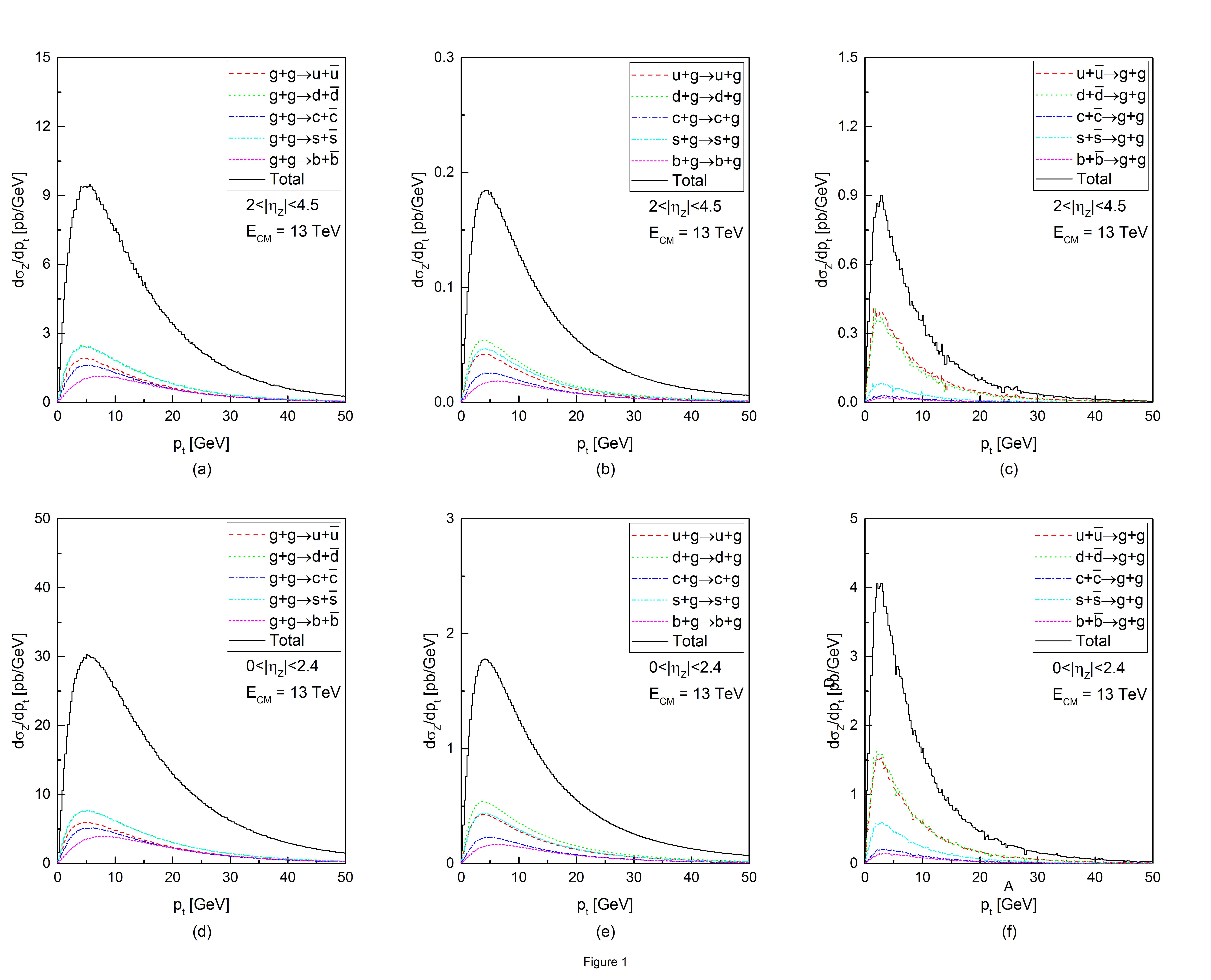
Figure 1: Contributions of the individual quark flavors into the differential cross-section of the productions of $Z^{0}$ boson in an inelastic collision at $E_{CM}=13\;TeV$, plotted as a function of the transverse momentum of the produced particle. The panels (a), (b) and (c) illustrate our calculations for the forward rapidity region, $2<|y_{Z}|<4.5$ (with the addition of $p_{t}^{\mu\bar{\mu}}>20\;GeV$ and $60<m^{\mu\bar{\mu}}<120\;GeV$ constraints, corresponding to the experimental measurements of the $LHCb$ collaboration, the reference LHCb ). The panels (d), (e) and (f) are our results in the central rapidity region, $0<|y_{Z}|<2.4$ (with the addition of $p_{t}^{\mu\bar{\mu}}>25\;GeV$ and $60<m^{\mu\bar{\mu}}<120\;GeV$ constraints, corresponding to the perlimanary measurements of the $CMS$ collaboration, the reference CMS ). The calculations are performed, using the $KMR$ $UPDF$ and the $PDF$ of $MMHT2014$.

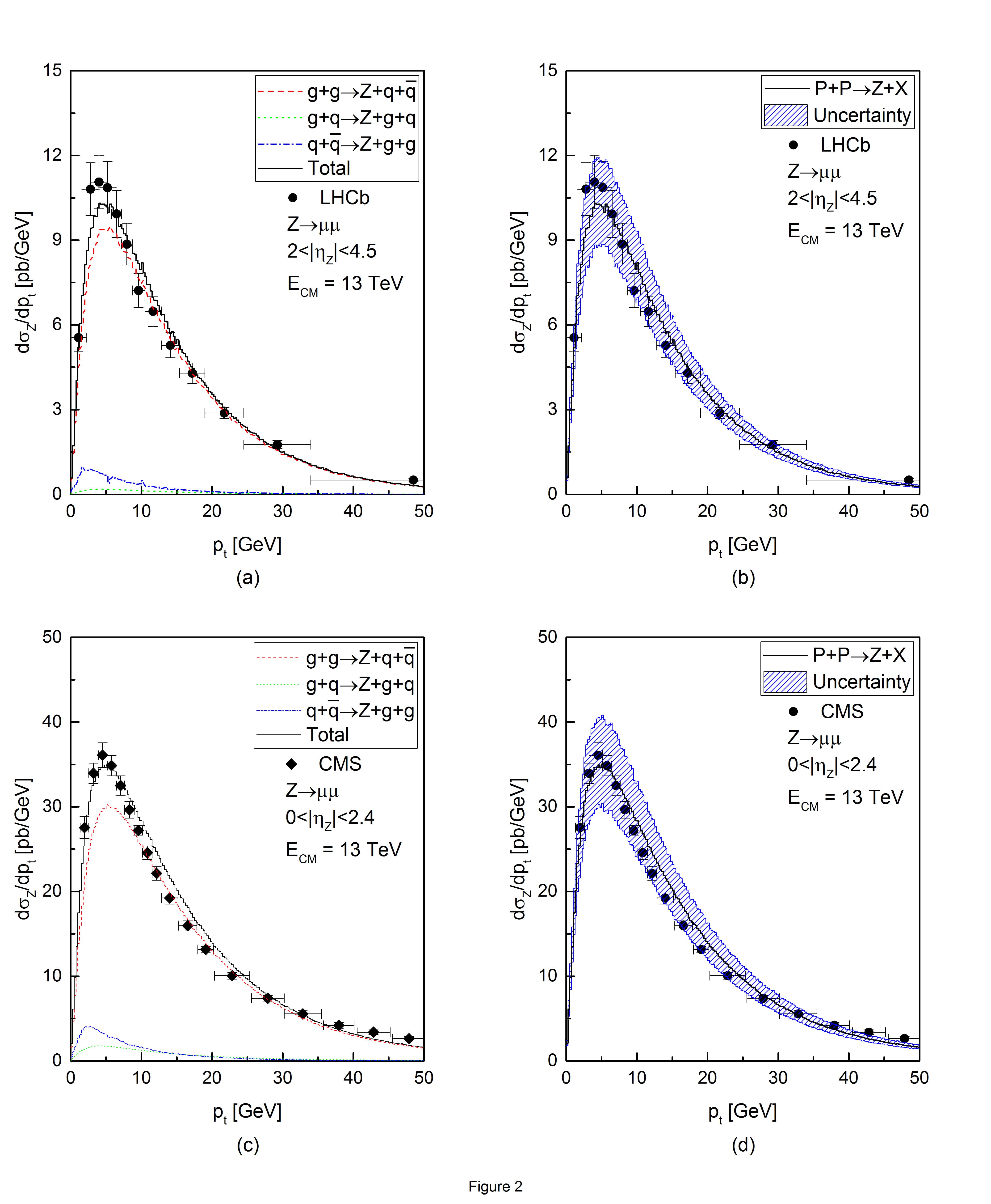
Figure 2: Differential cross-section of the productions of $Z^{0}$ boson as a function of the transverse momentum of the produced boson at $E_{CM}=13\;TeV$. Panels (a) and (c) illustrate the contributions from the individual sub-processes have been compared to each other in the respective rapidity regions. The panels (b) and (d) illustrate our results in their corresponding uncertainty bounds, compared to the data of the $LHCb$ and the $CMS$ collaborations, the references LHCb ; CMS . The uncertainty bounds have been calculated, by manipulating the hard-scale of the $UPDF$ by a factor of 2.

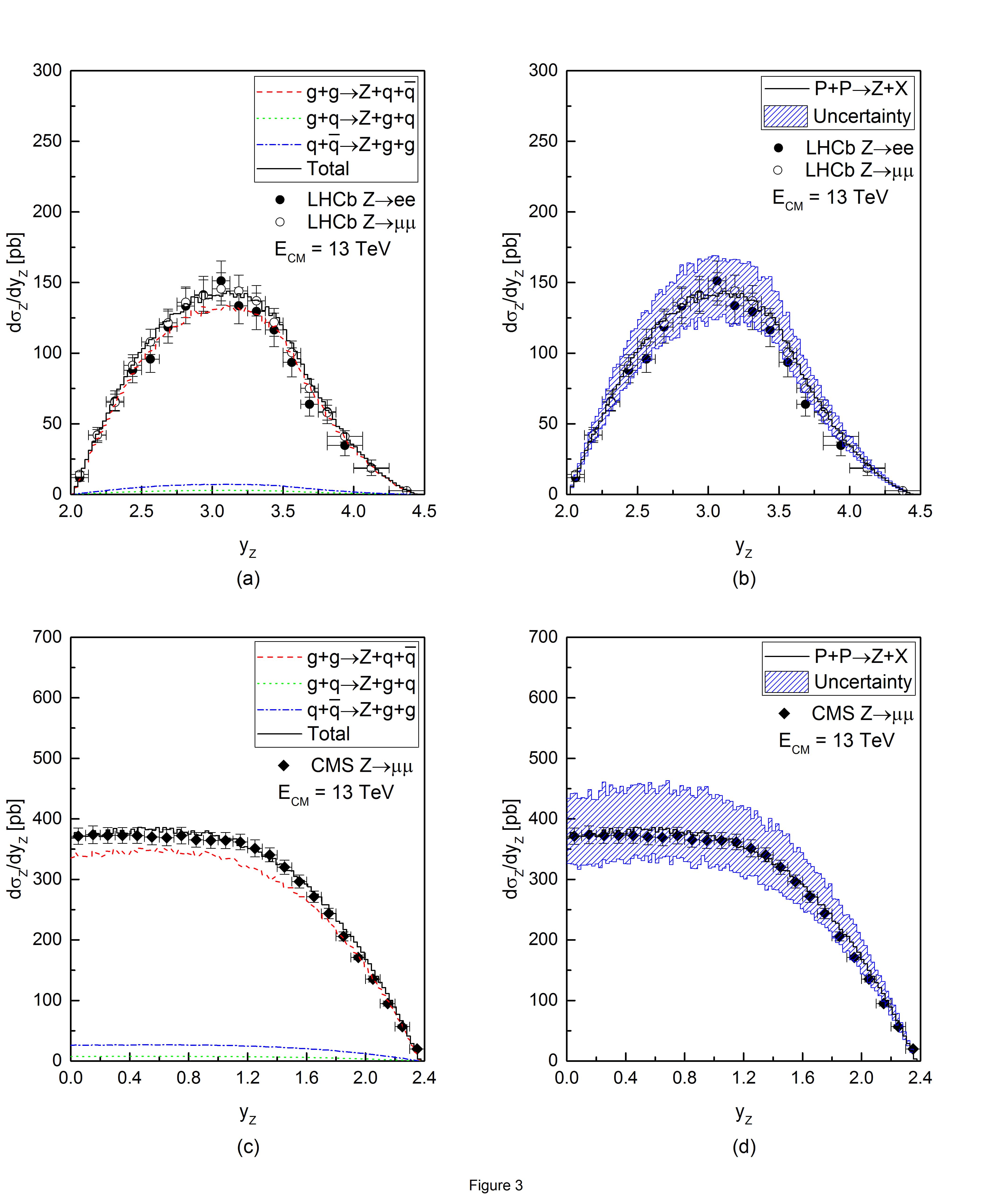
Figure 3: Differential cross-section of the productions of $Z^{0}$ boson as a function of the rapidity of the produced boson at $E_{CM}=13\;TeV$. The notions of the diagrams are the same as in the figure 2.

- (1) LHCb collaboration, R. Aaij et al., JHEP 06 (2012) 058.
- (2) LHCb collaboration, R. Aaij et al., JHEP 02 (2013) 106.
- (3) LHCb collaboration, R. Aaij et al., JHEP 08 (2015) 039.
- (4) LHCb collaboration, JHEP 05 (2015) 109, arXiv:1503.00963.
- (5) LHCb collaboration, R. Aaij et al., JHEP 01 (2015) 155.
- (6) ATLAS Collaboration, Phys.Rev.Lett. 109 (2012) 012001.
- (7) ATLAS Collaboration, Phys.Rev.D 91 (2015) 052005.
- (8) ATLAS Collaboration, Georges Aad et al., Eur. Phys. J. C 76(5) (2016) 1-61.
- (9) CMS Collaboration, J. High Energy Phys. 10 (2011) 132, doi:10.1007/JHEP10(2011)132.
- (10) CMS Collaboration, Vardan Khachatryan et al., phys.Lett.B 749 (2015) 187.
- (11) LHCb collaboration, R. Aaij et al., JHEP 09 (2016) 136.
- (12) CMS collaboration, CMS PAS SMP-15-011.
- (13) M. Modarres, M.R. Masouminia, R. Aminzadeh-Nik et al., accepted for publication in Phys.Rev.D, arXiv:1609.07920.
- (14) M.A. Kimber, A.D. Martin and M.G. Ryskin, Phys.Rev.D, 63 (2001) 114027.
- (15) A.D. Martin, M.G. Ryskin, G. Watt, Eur.Phys.J.C, 66 (2010) 163.
- (16) F. Abe et al. (CDF Collaboration), Phys.Rev.Lett., 76 (1996) 3070.
- (17) B. Affolder et al. (CDF Collaboration), Phys.Rev.Lett., 84 (2000) 845.
- (18) S. Abachi et al. (D0 Collaboration), Phys.Rev.Lett., 75 (1995) 1456.
- (19) B. Abbott et al. (D0 Collaboration), Phys.Rev.Lett., 80 (1998) 5498.
- (20) B. Abbott et al. (D0 Collaboration), Phys.Rev.D, 61 (2000) 072001.
- (21) B. Abbott et al. (D0 Collaboration), Phys.Rev.D, 61 (2000) 032004.
- (22) B. Abbott et al. (D0 Collaboration), Phys.Lett.B, 513 (2001) 292.
- (23) V.N. Gribov and L.N. Lipatov, Yad. Fiz., 15 (1972) 781.
- (24) L.N. Lipatov, Sov.J.Nucl.Phys., 20 (1975) 94.
- (25) G. Altarelli and G. Parisi, Nucl.Phys.B, 126 (1977) 298.
- (26) Y.L. Dokshitzer, Sov.Phys.JETP, 46 (1977) 641.
- (27) M. Modarres, H. Hosseinkhani, Nucl.Phys.A, 815 (2009) 40.
- (28) M. Modarres, H. Hosseinkhani, Few-Body Syst., 47 (2010) 237.
- (29) H. Hosseinkhani, M. Modarres, Phys.Lett.B, 694 (2011) 355.
- (30) H. Hosseinkhani, M. Modarres, Phys.Lett.B, 708 (2012) 75.
- (31) M. Modarres, H. Hosseinkhani, N. Olanj, Nucl.Phys.A, 902 (2013) 21.
- (32) M. Modarres, H. Hosseinkhani and N. Olanj, Phys.Rev.D, 89 (2014) 034015.
- (33) M. Modarres, H. Hosseinkhani, N. Olanj, M.R. Masouminia, Eur.Phys.J.C, 75 (2015) 556.
- (34) M. Modarres, M.R. Masouminia, H. Hosseinkhani, N. Olanj, Nucl.Phys.A, 945 (2016) 168185.
- (35) M.A. Kimber, A.D. Martin and M.G. Ryskin, Eur.Phys.J.C 12 (2000) 655.
- (36) L. A. Harland-Lang, A. D. Martin, P. Motylinski, R.S. Thorne, Eur.Phys.J.C, 75 (2015) 204.
- (37) S. P. Baranov, A.V. Lipatov, and N. P. Zotov, Phys.Rev.D, 78 (2008) 014025.
- (38) S.P. Baranov, A.V. Lipatov and N.P. Zotov, Phys.Rev.D, 81 (2010) 094034.
- (39) A.V. Lipatov and N.P. Zotov, Phys.Rev.D, 81 (2010) 094027; Phys.Rev.D, 72 (2005) 054002.
- (40) M. Deak, Transversal momentum of the electroweak gauge boson and forward jets in high energy factorization at the LHC, Ph.D thesis, University of Humburg, germany, 2009.
- (41) W. Furmanski, R. Petronzio, Phys.Lett.B, 97 (1980) 437.
- (42) G. P. Lepage, J. Comput. Phys. 27 (1978) 192 .
- (43) G. Watt, A.D. Martina and M.G. Ryskina, Phys.Rev.D 70 (2004) 014012.