Singularity-free Numerical Scheme for the Stationary Wigner Equation

Abstract

For the stationary Wigner equation with inflow boundary conditions, its numerical convergence with respect to the velocity mesh size are deteriorated due to the singularity at velocity zero. In this paper, using the fact that the solution of the stationary Wigner equation is subject to an algebraic constraint, we prove that the Wigner equation can be written into a form with a bounded operator $\mathcal{B}[V]$, which is equivalent to the operator $\mathcal{A}[V]=\Theta[V]/v$ in the original Wigner equation under some conditions. Then the discrete operators discretizing $\mathcal{B}[V]$ are proved to be uniformly bounded with respect to the mesh size. Based on the therectical findings, a signularity-free numerical method is proposed. Numerical reuslts are proivded to show our improved numerical scheme performs much better in numerical convergence than the original scheme based on discretizing $\mathcal{A}[V]$.

Keywords: stationary Wigner equation; singularity-free; numerical convergence;

1 Introduction

The Wigner transport equation is one of the quantum mechanical frameworks. It is proposed by E. Wigner in 1932 as a quantum correction to the classical statistical mechanics[25]. Though the Wigner function may take negative values, it has a non-negative marginal distribution and can express system observables in the same way as the Boltzmann probability density function, thus it is called a quasi-probability density function. The strong similarity between the Wigner equation and the Boltzmann equation makes it convenient to borrow some describing tools of the latter, e.g., the boundary conditions and the scattering terms[7].

The Wigner equation has been used in many fields. For example, Frensley successfully reproduced the negative differential resistance phenomena of resonant tunneling devices by numerically solving the following one-dimensional Wigner equation

$$\frac{\partial f}{\partial t}+v\frac{\partial f}{\partial x}-\Theta[V]f=0,x\in(-l/2,l/2),v\in\mathbb{R},$$ (1)

with inflow boundary conditions

$$f(-l/2,v)=f_{l}(v),\text{ if }v>0;f(l/2,v)=f_{r}(v),\text{ if }v<0.$$ (2)

$\Theta[V]$ is a pseudo-differential operator that will be explained later. Since then, the Wigner equation has attracted many researchers in numerical simulation (e.g., [15] and references therein), and various numerical methods for the Wigner equation have been proposed, such as finite difference methods [8, 12, 4, 13], spectral methods [24, 22, 4], spectral element method [24], and Monte Carlo methods[20, 23]. When the Hartree potential is included, the Wigner-Poisson system self-consistently can be solved [5, 11, 2, 27, 17]. The nonlinear iteration for the coupled Wigner-Poisson system deserves a serious study and in [4] the Gummel method and the Newton method were compared for the RTD simulation in terms of efficiency, accuracy and robustness. As for the linear stationary Wigner equation with inflow boundary boundary conditions, there are still a lot of open problems, for example, the well-posedness, the numerical convergence, etc. In this paper, we focus on the linear problem.

Many mathematicians have been drawn to study the Wigner equation, e.g., [21, 18, 9, 10, 19]. The existence and uniqueness of the solution for the Wigner equation have been proved by using of the theoretical result of the Schrödinger equation. But there are still a lot of open problems. One of them is to build the well-posedness result for the Wigner boundary value problem (the stationary Wigner equation with inflow boundary conditions), which is a popular model in numerical simulation of the nano semiconductor devices. We note that some researchers have proved the well-posedness of the Wigner boundary value problem in some special cases, for example, [1] for a velocity semi-discretization version, [3] for an approximate problem by removing a small interval centered at velocity zero, and [16] for a periodical potential.

It is pointed out that the Wigner BVP problem is more difficult than the Wigner initial value problem, and one of the reason is that the inflow boundary conditions break up the equivalence between the Wigner equation and the Schrödinger equation. When using a numerical methods to discretize the Wigner equation, computational parameters such the mesh size and the correlation length are sensitive and need a careful calibration [27]. In [14], several numerical schemes including first-order (FDS) and second-order difference schemes (SDS) for discretization of the advection term $v\frac{\partial f}{\partial x}$ of the Wigner equation were compared. However, to authors’ knowledge, a detailed accuracy study of the finite difference methods for the Wigner BVP with respect to the velocity mesh size has not been reported. One of the difficulties is that the operator $\frac{1}{v}\Theta[V]$ is singular at $v=0$, which results in the numerical solution’s oscillation and blowing up as the velocity mesh size goes to zero. Assuming that the Wigner BVP has a unique smooth solution, we observe that the solution must satisfy $(\Theta[V]f)(x,0)=0$. In this paper, we design a new numerical scheme by applying this constraint in our numerical scheme.

The rest of the paper is arranged as follows. In Section 2, we rewrite the original Wigner equaiton into a form with a bounded operator $\mathcal{B}[V]$ which is equivalent to $\mathcal{A}[V]$ under the assumption that the distribution function satsfies an algebraic constraint. In Section 3, we prove the discrete operators discretizing $\mathcal{B}[V]$ to be uniformly bounded with respect to the mesh size. Based on this analysis, a new numerical method is proposed. At last, in Section 4, we give some numerical examples to show the numerical convergence with respect to $x$-space and $v$-space. Some clonclusion remarks are given in last section.

2 Stationary Wigner equation and an equivalent form

We are concerned with the following stationary Wigner equation (or ”quantum Liouville equation ”)

$$v\frac{\partial f}{\partial x}=\Theta[V]f(x,v),$$ (3)

where $\Theta[V]$ is a pseudo-differential operator defined by

$$\Theta[V]f(x,v)=\int_{-\infty}^{\infty}V_{w}\left(x,v-v^{\prime}\right)f\left(x,v^{\prime}\right)dv^{\prime}.$$ (4)

$V_{w}(x,v)$ is called the Wigner potential and defined by

$$V_{w}\left(x,v\right)=\frac{i}{2\pi}\int_{-\infty}^{\infty}D_{V}(x,y)\exp\left(ivy\right)\mathrm{dy},$$ (5)

where

$$D_{V}(x,y)=V\left(x+y/2\right)-V\left(x-y/2\right)$$

is the difference of the potential $V$ at positions $x+y/2$ and $x-y/2$. $\Theta[V]$ can be proved to be a a continuous (bounded) linear operator on $L^{2}(\mathbb{R})$ if $V\in L^{\infty}(\mathbb{R})$.

In this paper, we use the Fourier transform and its corresponding inverse defined as

$$\hat{f}(y)=\mathcal{F}(f)=\int_{-\infty}^{\infty}f(v)\exp(-ivy)\,\mathrm{d}v,$$ (6)

$$f(v)=\mathcal{F}^{-1}(\hat{f})=\frac{1}{2\pi}\int_{-\infty}^{\infty}\hat{f}(y)\exp(ivy)\,\mathrm{d}y.$$ (7)

In the sense of Fourier transform, $\Theta[V]$ can also be written as

$$\Theta[V]f(v)=V_{w}\ast f(v)=i\mathcal{F}^{-1}(D_{V})\ast\mathcal{F}^{-1}(\hat{f})=i\mathcal{F}^{-1}(D_{V}\hat{f}),$$ (8)

where $\ast$ denotes convolution. By the Parseval equality, we have

$$\|\Theta[V]f\|_{2}=\frac{1}{2\pi}\|D_{V}\hat{f}\|_{2}\leqslant 2\cdot\frac{1}{2\pi}\|V\|_{\infty}\cdot\|\hat{f}\|_{2}=2\|V\|_{\infty}\cdot\|f\|_{2}.$$ (9)

Immediately, we have the following lemma.

Lemma 1.

Suppose that the potential $V\in L^{\infty}(\mathbb{R})$. For any $x\in\mathbb{R}$, the operator $\Theta[V]$ is a bounded linear operator on $L^{2}(\mathbb{R}_{v})$, and

$$\|\Theta[V]\|\leqslant 2\|V\|_{\infty}.$$

Dividing (3) by $v$ gives

$$\dfrac{\partial{f}}{\partial{x}}=\mathcal{A}[V]f(x,v)$$ (10)

where the operator $\mathcal{A}[V]$ is defined by

$$\mathcal{A}[V]f(x,v)=\frac{1}{v}\Theta[V]f(x,v)=\dfrac{1}{v}\int_{-\infty}^{\infty}V_{w}(x,v-v^{\prime})f(x,v^{\prime})\,\mathrm{d}v^{\prime}.$$ (11)

The equation (10) can be viewed as an evolution system, which gives us a convenient way to analyze and compute the stationary Wigner equation. However, $\frac{V_{w}(x,v-v^{\prime})}{v}$, the kernel of $\mathcal{A}[V]$, is singular at $v=0$, and this brings great difficulty to solve and analyze (10). Although we usually avoid the point at ”$v=0$” to be a mesh point in numerical experiments, the numerical distribution can suffer from severe oscillation when using a small velocity mesh size. It is a reason that no numerical convergence work has been published.

Under the condition that $f(x,v)$ is Lipschitz continuous with respect to $x$ which ensures the boundedness of $\dfrac{\partial{f(x,v)}}{\partial{x}}$, setting $v=0$ in (3) yields

$$\int V_{w}\left(x,-v^{\prime}\right)f\left(x,v^{\prime}\right)dv^{\prime}=0.$$ (12)

This is an important property of the stationary Wigner equation, which will be used to design a numerical method. Subtracting (12) from (3), we obtain

$$v\frac{\partial f}{\partial x}=\int\left[V_{w}\left(x,v-v^{\prime}\right)-V_{w}\left(x,v\right)\right]f\left(x,v^{\prime}\right)dv^{\prime}.$$ (13)

Then we divide the above equation by $v$, and obtain

$$\frac{\partial f}{\partial x}=\mathcal{B}[V]f(x,v),$$ (14)

where the operator $\mathcal{B}[V]$ is defined as

$$\mathcal{B}[V]f(x,v)=\int\frac{V_{w}\left(x,v-v^{\prime}\right)-V_{w}\left(x,-v^{\prime}\right)}{v}f(x,v^{\prime})dv^{\prime}.$$ (15)

Equation (14)-(15) is equivalent to the stationary Wigner equation if (12) holds.

Now we focus on the properties of the operator $\mathcal{B}[V]$. It is evident that the operator $\mathcal{B}[V]$ is different from $\mathcal{A}[V]$. But they are equal on some special spaces, e.g., $f(x,v)$ is an even function with respect to $v$. We will prove that $\mathcal{B}[V]$ is a bounded linear operator under some assumptions. The details are shown in the following Theorem 1.

Theorem 1.

Suppose that for any $x\in[-l/2,l/2]$, the Wigner potential $V_{w}(x,\cdot)$ defined in (5) belongs to $H^{1}(\mathbb{R}_{v})$. Then $\mathcal{B}[V]:L^{2}(\mathbb{R}_{v})\to L^{2}(\mathbb{R}_{v})$ is a bounded linear operator.

Proof.

For any $f\in L^{2}(\mathbb{R}_{v})$,

$$\|\mathcal{B}[V]f\|_{L^{2}(\mathbb{R}_{v})}^{2}=\int_{-\infty}^{\infty}|\mathcal{B}[V]f|^{2}\,\mathrm{d}v.$$ (16)

We will prove the boundedness of $\mathcal{B}[V]$ by estimating (16) on the region $|v|>1$ and the region $|v|\leqslant 1$ respectively.

First, we consider the part with $\left|v\right|>1$. Using $V_{w}\left(x,v\right)\in L^{2}\left(\mathbb{R}_{v}\right)$ and the Young’s inequality, we have

$$\left\|\Theta[V]f(x,v)\right\|_{L^{\infty}(\mathbb{R}_{v})}=\|V_{w}\left(x,v\right)\ast f\left(v\right)\|_{L^{\infty}\left(\mathbb{R}_{v}\right)}\leq\|V_{w}\left(v\right)\|_{L^{2}(\mathbb{R}_{v})}\|f\left(v\right)\|_{L^{2}\left(\mathbb{R}_{v}\right)}.$$ (17)

By the Cauchy-Schwartz inequality, we then have

$$\left|\int_{\mathbb{R}_{v^{\prime}}}V_{w}\left(x,0-v^{\prime}\right)f\left(x,v^{\prime}\right)\,\mathrm{d}v^{\prime}\right|\leq\|V_{w}\left(x,v\right)\|_{L^{2}(\mathbb{R}_{v})}\|f\left(x,v\right)\|_{L^{2}\left(\mathbb{R}_{v}\right)}.$$ (18)

It is obtained directly from (17) and (18) that

$$\qquad\int_{\left|v\right|>1}\left|\mathcal{B}[V]f(x,v)\right|^{2}\,\mathrm{d}v$$

$$\leqslant 2\int_{\left|v\right|>1}\left|\frac{\Theta[V]f\left(x,v\right)}{v}\right|^{2}\,\mathrm{d}v+2\int_{\left|v\right|>1}\frac{\|V_{w}\left(x,\cdot\right)\|_{L^{2}(\mathbb{R}_{v})}^{2}\|f\left(x,\cdot\right)\|_{L^{2}\left(\mathbb{R}_{v}\right)}^{2}}{v^{2}}\,\mathrm{d}v$$

$$\leqslant 8\|V_{w}\left(x,v\right)\|^{2}_{L^{2}(\mathbb{R}_{v})}\|f\left(x,v\right)\|^{2}_{L^{2}(\mathbb{R}_{v})}.$$ (19)

Then, we consider the part with $\left|v\right|\leqslant 1$. According to the Cauchy-Schwartz inequality again, we have

$$\left|\mathcal{B}[V]f(x,v)\right| \leqslant\int_{\mathbb{R}}\left|\frac{V_{w}\left(x,v-v^{\prime}\right)-V_{w}\left(x,0-v^{\prime}\right)}{v}\right|\left|f\left(x,v^{\prime}\right)\right|\,\mathrm{d}v^{\prime}$$

$$\leqslant\left\|\frac{V_{w}\left(x,v-v^{\prime}\right)-V_{w}\left(x,0-v^{\prime}\right)}{v}\right\|_{L^{2}\left(\mathbb{R}_{v^{\prime}}\right)}\|f\left(x,\cdot\right)\|_{L^{2}(\mathbb{R}_{v})},\quad v\in\left[-1,1\right].$$

By using Theorem 3 in Chapter 5 of [6], we have

$$\left\|\frac{V_{w}\left(x,v-v^{\prime}\right)-V_{w}\left(x,-v^{\prime}\right)}{v}\right\|_{L^{2}\left(\mathbb{R}_{v^{\prime}}\right)}\leqslant\left\|\partial_{v^{\prime}}V_{w}\left(x,v^{\prime}\right)\right\|_{L^{2}\left(\mathbb{R}_{v^{\prime}}\right)}.$$

This fact, together with the Cauchy-Schwartz inequality, gives us the following estimate on the velocity interval $[-1,1]$ that

$$\int_{\left|v\right|\leq 1}\left|\mathcal{B}[V]f(x,v)\right|^{2}\,\mathrm{d}v\leq\|f\left(x,v\right)\|^{2}_{L^{2}(\mathbb{R}_{v})}\left\|\partial_{v}V_{w}\left(x,v\right)\right\|^{2}_{L^{2}\left(\mathbb{R}_{v}\right)}$$ (20)

Collecting (19) and (20) together results in

$$\|\mathcal{B}[V]f(x,v)\|^{2}_{L^{2}(\mathbb{R}_{v})}\leqslant C\|f\left(x,v\right)\|^{{}^{2}}_{L^{2}(\mathbb{R}_{v})}$$

where

$$C=8\left\|V_{w}\left(x,v\right)\right\|^{{}^{2}}_{H^{1}(\mathbb{R}_{v})}.$$

This completes the proof that $\mathcal{B}[V]$ is a bounded linear operator on $L^{2}(\mathbb{R}_{v})$.

∎

We have proved the operator $\mathcal{B}[V]$ is bounded, thus obtained a singularity-free form (14)-(15), which is euquivalent to the original Wigner equation. A numerical scheme based on the singularity-free from will be porposed in the next section.

3 Singularity-free numerical scheme

We start from the discretization of the pseudo-differential operator $\Theta[V]$, then define the corresponding discrete operators of $\mathcal{A}[V]=\frac{1}{v}\Theta[V]$ and $\mathcal{B}[V]$, respectively. At the end of this section, we prove that the discrete operators of $\mathcal{B}[V]$ is uniformly bounded with respect to the velocity mesh size.

Before introducing the discretization of the pseudo-differential operator $\Theta[V]$, we define a new operator $\Theta^{h}[V]:L^{2}(\mathbb{R}_{v})\to L^{2}(\mathbb{R}_{v})$, the approximation of $\Theta[V]$,

$$\Theta^{h}[V](f) = i\mathcal{F}^{-1}_{y\rightarrow v}\left(D_{V}\chi_{|y|\leqslant R^{h}}\hat{f}(y)\right),\qquad\forall f\in L^{2}(\mathbb{R}_{v}),$$ (21)

where $\chi_{|y|\leqslant R^{h}}$ is the characteristic function of $\{y:|y|\leqslant R^{h}\}$. Here $h$ is related to the velocity mesh size ($\Delta v=2\pi h$), and $R^{h}$ is related to $h$ by

$$R^{h}=\frac{1}{2h}.$$ (22)

In some papers, e.g., [8], $R^{h}$ is called the coherence length. We introduce a subspace $L^{2}_{h}(\mathbb{R})$ of $L^{2}(\mathbb{R})$ defined as

$$L^{2}_{h}(\mathbb{R})=\left\{g\in L^{2}(\mathbb{R})|\text{supp}\hat{g}\subset[-R^{h},R^{h}]\right\}.$$ (23)

For any function $f^{h}\in L^{2}_{h}(\mathbb{R})$, by using the Shannon sampling theorem, we have

$$f^{h}(v)=\sum_{n=-\infty}^{\infty}f_{n}\text{sinc}\left(\frac{v-v_{n}}{2h}\right),$$ (24)

where

$$\text{sinc}(x):=\dfrac{\sin x}{x},$$ (25)

and

$$f_{n}=f^{h}(v_{n}),v_{n}=(2n+1)\pi h,\ n\in\mathbb{Z}.$$ (26)

$\{v_{n}:n\in\mathbb{Z}\}$are the sampling velocity points, and the series is absolutely and uniformly convergent on compact sets [26]. Actually,

$$\int_{\mathbb{R}_{v}}\text{sinc}(\frac{v-v_{n}}{2h})\text{sinc}(\frac{v-v_{m}}{2h})\,\mathrm{d}v=\begin{cases}2\pi h,&\text{if }n=m,\\ 0,&\text{else,}\end{cases}$$ (27)

and $\left\{\text{sinc}(\frac{v-v_{n}}{2h}):n\in\mathbb{Z}\right\}$ is an orthogonal basis of $L^{2}_{h}(\mathbb{R})$. From (24), we can define an isometry (disregarding a constant) $\mathcal{I}_{h}:L^{2}_{h}(\mathbb{R})\rightarrow l^{2}(\mathbb{Z})$: for any $f^{h}\in L^{2}_{h}(\mathbb{R})$,

$$\mathcal{I}_{h}f^{h}=(\cdots,f_{-1},f_{0},f_{1},\cdots)^{T}$$ (28)

where $\left\{f_{n}\right\}$ is defined in (26). It is easy to see that

$$\|\mathcal{I}_{h}f^{h}\|_{l^{2}(\mathbb{Z})}=\frac{1}{\sqrt{2\pi h}}\|f^{h}\|_{L^{2}(\mathbb{R})}.$$ (29)

$\Theta^{h}[V]$ can be considered as the restriction of $\Theta[V]$ on $L^{2}_{h}(\mathbb{R})$, and there are some obvious properties for the operator $\Theta^{h}[V]$, showing in Property 1.

Property 1.

The approximated operator $\Theta^{h}[V]$ fulfills the following properties:

1. if $f\in L^{2}_{h}(\mathbb{R})$, then $\Theta^{h}[V](f)=\Theta[V](f)$;

2. if $f\in L^{2}(\mathbb{R})$, then $\Theta^{h}[V](f)$ converges to $\Theta[V](f)$ in $L^{2}(\mathbb{R})$ as $h\rightarrow 0$. If, furthermore, $f$ lies in the Soblev space $H^{s}(\mathbb{R})$, $s>0$, we get

   $$\|\Theta^{h}[V](f)-\Theta[V](f)\|^{2}_{L^{2}(\mathbb{R})}\leqslant\dfrac{4\|V\|_{\infty}}{2\pi}\dfrac{\|f\|^{2}_{H^{s}_{\mathbb{R}}}}{\left(1+(R^{h})\right)^{s}}.$$

We consider the discretization of $\Theta[V]f$ in the Wigner equation for $f(x,v)$ assuming that $f(x,v)\in L^{2}(\mathbb{R}),\forall x\in[-l/2,l/2]$. We use $f_{n}(x)$ to represent the numerical approximation of $f(x,v_{n})$, and ${\bf{f}}=\{f_{n}:n\in\mathbb{Z}\}\in l^{2}(\mathbb{Z})$. Based on Property 1 and the Shannon sampling theorem, a discrete operator $\Theta_{d}[V]:l^{2}(\mathbb{Z})\rightarrow l^{2}(\mathbb{Z})$ as an approximation of $\Theta[V]$ on $L^{2}(\mathbb{R})$ can be constructed by

$$\Theta_{d}[V]{\bf{f}}=\mathcal{I}_{h}\Theta^{h}[V]\mathcal{I}^{-1}_{h}{\bf{f}}=2\pi hM^{\Theta_{d}}{\bf{f}}$$ (30)

where $\mathcal{I}_{h}$ is defined in (28), $\mathcal{I}_{h}^{-1}$ is the inverse of $\mathcal{I}_{h}$, and $M^{\Theta_{d}}$ is an infinite dimensional matrix with

$$M^{\Theta_{d}}_{nm}=\frac{{\rm{i}}}{2\pi}\int_{\mathbb{R}}D_{V}(x,y)\chi_{(-R^{h},R^{h})}(y)e^{{\rm{i}}(v_{n}-v_{m})y}\,\mathrm{d}y.$$ (31)

$M^{\Theta_{d}}$ is the matrix of a discrete convolution operator and $M^{\Theta_{d}}_{nm}$ depends only on $n-m$. And $M^{\Theta_{d}}$ is a real-valued skew-symmetric matrix, i.e., $M^{\Theta_{d}}_{nm}=-M^{\Theta_{d}}_{mn}$.

We are able to establish a property for the operator $\Theta_{d}[V]$, which is the discrete analogue of Lemma 1.

Property 2.

The operator $\Theta_{d}$ is a bounded linear operator on $\ell^{2}$, and its norm is estimated uniformly with respect to $h$ by $\|\Theta_{d}\|_{\mathcal{L}(\ell^{2})}\leqslant 2\|V\|_{\infty}$.

A typical semi-discretization of the orignal stationary Wigner equation with inflow boundary conditions can be written as

$$\left\{\begin{array}[]{ll}\dfrac{\,\mathrm{d}{{\bf{f}}}}{\,\mathrm{d}{x}}=\mathcal{A}_{d}[V]{\bf{f}},&x\in(-l/2,l/2),\\ f_{n}(-l/2)=f_{L}(v_{n}),&\mathrm{if}\ v_{n}>0,\\ f_{n+1/2}(l/2)=f_{R}(v_{n}),&\mathrm{if}\ v_{n}<0,\\ \end{array}\right.$$ (32)

where the operator $\mathcal{A}_{d}[V]:l^{2}\rightarrow l^{2}$ is defined by

$$(A_{d}[V]{\bf{f}})_{n}=\frac{1}{v_{n}}(\Theta_{d}[V]{\bf{f}})_{n},$$

where $\Theta_{d}[V]$ is defined in (30). $A_{d}[V]$ is obviously bounded, but its norm will grow to infinity as the velocity mesh size $h\rightarrow 0$. The property makes the numerical solution suffer from numerical instability when a small velocity mesh size $h$ is used, and it also affects the numerical convergence of the numerical solution.

Based on the equivalent singularity-free form (14)-(15), we can derive a semi-discretization scheme for the stationary Wigner equation with inflow boundary conditions

$$\left\{\begin{array}[]{ll}\dfrac{\,\mathrm{d}{{\bf{f}}}}{\,\mathrm{d}{x}}=\mathcal{B}_{d}[V]{\bf{f}},&x\in(-l/2,l/2),\\ f_{n}(-l/2)=f_{L}(v_{n}),&\mathrm{if}\ v_{n}>0,\\ f_{n+1/2}(l/2)=f_{R}(v_{n}),&\mathrm{if}\ v_{n}<0,\\ \end{array}\right.$$ (33)

Here the discrete operator $\mathcal{B}_{d}[V]:l^{2}\rightarrow l^{2}$ is obtained by discretization of the bounded operator $\mathcal{B}[V]$, and can be written out as

$$\left(\mathcal{B}_{d}[V]{\bf{f}}\right)_{n}=\frac{2\pi h}{v_{n}}\sum_{m\in\mathbb{Z}}(M^{\Theta_{d}}_{nm}-a_{m})f_{m},$$ (34)

where $M^{\Theta_{d}}_{nm}$ is given in (31) and

$$a_{m}=\frac{{\rm{i}}}{2\pi}\int_{\mathbb{R}}D_{V}(x,y)\chi_{(-R^{h},R^{h})}(y)e^{-{\rm{i}}v_{m}y}\,\mathrm{d}y.$$ (35)

We will prove $\mathcal{B}_{d}[V]$ is uniformly bounded with some assumptions of the potential $V$ in the following theorem.

Theorem 2.

Suppose that $V_{w}(x,\cdot)\in H^{1}(\mathbb{R}_{v})$ for any $x\in[-l/2,l/2]$. For a given velocity mesh size $h>0$, we define $\mathcal{B}_{d}[V]:l^{2}(\mathbb{Z})\rightarrow l^{2}(\mathbb{Z})$ as in (34) where $v_{n}=(2n+1)\pi h$. Then $\mathcal{B}_{d}[V]$ is uniformly bounded i.e., $\|\mathcal{B}_{d}[V]\|\leq C$ where $C$ does not depend on the velocity mesh size $h$ or $x$.

Proof.

The proof is similar to that of Theorem 1. First, we consder $|v_{n}|\leqslant 1$. For $\mathbf{g}=\{g_{n}:n\in\mathbb{Z}\}\in l^{2}(\mathbb{Z})$, we can write $n$th-component of $\mathcal{B}_{d}[V]\mathbf{g}$ as

$$(\mathcal{B}_{d}[V]\mathbf{g})_{n}={\rm{i}}h\sum_{m\in\mathbb{Z}}g_{m}\int_{-\frac{1}{2h}}^{\frac{1}{2h}}D_{V}(x,y)\frac{e^{{\rm{i}}(v_{n}-v_{m})y}-e^{-{\rm{i}}v_{m}y}}{v_{n}}\,\mathrm{d}y.$$ (36)

by using (34), (31) and (22).

For each $v_{n}$, we introduce a vector $\mathbf{q}^{v_{n}}=\left\{q_{m}^{v_{n}}:m\in\mathbb{Z}\right\}$ defined as

$$q_{m}^{v_{n}}=-h\int_{-\frac{1}{2h}}^{\frac{1}{2h}}yD_{V}(x,y)\text{sinc}\frac{v_{n}y}{2}e^{{\rm{i}}(\frac{v_{n}}{2}-v_{m})y}\,\mathrm{d}y.$$ (37)

So $(\mathcal{B}_{d}[V]\mathbf{g})_{n}$ in (36) can be written as the $l^{2}(\mathbb{Z})$ inner product of $\mathbf{q}^{v_{n}}$ and $\mathbf{g}$, i.e.,

$$(\mathcal{B}_{d}[V]\mathbf{g})_{n}=\left(\mathbf{q}^{v_{n}},\mathbf{g}\right)_{l^{2}(\mathbb{Z})}.$$ (38)

Applying the Cauchy-Schwartz inequality to (38), we have

$$|(\mathcal{B}_{d}[V]\mathbf{g})_{n}|\leqslant\|\mathbf{q}^{v_{n}}\|_{l^{2}(\mathbb{Z})}\|\mathbf{g}\|_{l^{2}(\mathbb{Z})}.$$ (39)

By using the Parseval theorem on (37), we have

$$\begin{split}\sum_{m\in\mathbb{Z}}|q_{m}^{v_{n}}|^{2}&=h\int_{-\frac{1}{2h}}^{\frac{1}{2h}}|\chi_{(-R^{h},R^{h})}(y)yD_{V}(x,y)\text{sinc}\frac{v_{n}y}{2}|^{2}\,\mathrm{d}y\\ &\leqslant h\int_{\mathbb{R}}|yD_{V}(x,y)|^{2}\,\mathrm{d}y\leqslant 2\pi h\|V_{w}(x,\cdot)\|_{H^{1}(\mathbb{R}_{v})}^{2}.\end{split}$$ (40)

The last $\leqslant$ is obtained by using the definition of $V_{w}(x,v)$ in (5). From (39) and (40), we conclude that $\{|(\mathcal{B}_{d}[V]\mathbf{g})_{n}|:n\in\mathbb{Z}\}$ is bounded, i.e.,

$$|(\mathcal{B}_{d}[V]\mathbf{g})_{n}|\leqslant\sqrt{2\pi h}\|V_{w}(x,\cdot)\|_{H^{1}(\mathbb{R}_{v})}\|\mathbf{g}\|_{l^{2}(\mathbb{Z})},\forall n\in\mathbb{Z}.$$ (41)

The number of $n$ such that $|v_{n}|\leqslant 1$ is less than $\frac{1}{\pi h}$, so we have

$$\sum_{\{n\in\mathbb{Z}:|(2n+1)\pi h|\leqslant 1\}}|(\mathcal{B}_{d}[V]\mathbf{g})_{n}|^{2}\leqslant 2\|V_{w}(x,\cdot)\|_{H^{1}(\mathbb{R}_{v})}^{2}\|\mathbf{g}\|_{l^{2}(\mathbb{Z})}^{2}.$$ (42)

Then we consider the case $|v_{n}|>1$. Different from (38), we rewrite (36) into

$$(\mathcal{B}_{d}[V]\mathbf{g})_{n}=\frac{1}{v_{n}}(\mathbf{\tilde{q}}^{v_{n}},\mathbf{g})_{l^{2}(\mathbb{Z})},$$ (43)

where $\mathbf{\tilde{q}}^{v_{n}}=\{\tilde{q}_{m}^{v_{n}}:m\in\mathbb{Z}\}$ and

$$\tilde{q}_{m}^{v_{n}}={\rm{i}}h\int_{\mathbb{R}}D_{V}(x,y)\chi_{(-R^{h},R^{h})}(y)(e^{{\rm{i}}v_{n}y}-1)e^{-{\rm{i}}v_{m}y}\,\mathrm{d}y.$$ (44)

Applying the Cauchy-Schwartz inequality to (43), we have

$$|(\mathcal{B}_{d}[V]\mathbf{g})_{n}|\leqslant\frac{1}{v_{n}}\|\mathbf{\tilde{q}}^{v_{n}}\|_{l^{2}(\mathbb{Z})}\|\mathbf{g}\|_{l^{2}(\mathbb{Z})}.$$ (45)

By using the Parseval theorem on (44), we have

$$\begin{split}\sum_{m\in\mathbb{Z}}|\tilde{q}_{m}^{v_{n}}|^{2}&=h\int_{\mathbb{R}}|D_{V}(x,y)\chi_{(-R^{h},R^{h})}(y)(e^{{\rm{i}}v_{n}y}-1)|^{2}\,\mathrm{d}y\\ &\leqslant 4h\int_{\mathbb{R}}|D_{V}(x,y)|^{2}\,\mathrm{d}y\\ &=4h\|D_{V}(x,\cdot)\|_{L^{2}(\mathbb{R})}^{2}\\ &=8\pi h\|V_{w}(x,\cdot)\|_{L^{2}(\mathbb{R})}^{2}.\end{split}$$ (46)

Plugging (46) into (45) yields the estimate

$$|(\mathcal{B}_{d}[V]\mathbf{g})_{n}|\leqslant\frac{2\sqrt{2\pi h}}{v_{n}}\|V_{w}(x,\cdot)\|_{L^{2}(\mathbb{R})}\|\mathbf{g}\|_{l^{2}(\mathbb{Z})}.$$ (47)

Recalling the relation between $\sum_{n\in\mathbb{Z},|v_{n}|>1}\frac{2\pi h}{|v_{n}|^{2}}$ and $\int_{|v|>1}\frac{1}{v^{2}}\,\mathrm{d}v$, we know that there exist a constant $C_{2}$ which does not depend on $h$ such that

$$\sum_{n\in\{n\in\mathbb{Z}:(2n+1)\pi h>1\}}|(\mathcal{B}_{d}[V]\mathbf{g})_{n}|^{2}\leqslant C_{2}\|V_{w}(x,\cdot)\|_{L^{2}(\mathbb{R}_{v})}^{2}\|\mathbf{g}\|_{l^{2}(\mathbb{Z})}^{2}.$$ (48)

Putting (42) and (48) together, we come to a conclusion that there exists a constant $C$ which does not dependent on $h$ such that

$$\sum_{n\in\mathbb{Z}}|(\mathcal{B}_{d}[V]\mathbf{g})_{n}|^{2}\leqslant C\|V_{w}(x,\cdot)\|_{H^{1}(\mathbb{R}_{v})}^{2}\sum_{m\in\mathbb{Z}}|g_{m}|^{2},$$ (49)

which completes the proof that $\mathcal{B}_{d}[V]$ is a uniformly bounded linear operator on $l^{2}$. ∎

We have proved that the discrete operators of the scheme based on the signularity-free stationary Wigner equation is uniformly bounded with respect to the velocity mesh size. So the numerical solution using the singularity-free scheme could be expected to have a better performance. In the next section, we will validate this by providing some numerical examples.

4 Numerical Examples

We consider a potential $V(x)$ given as

$$\begin{array}[]{l}V\left(x\right)=\left\{\begin{array}[]{ll}0,&\mathrm{if}\ x\notin\left[-1.5,1.5\right],\\ 0.2,&\mathrm{if}\ x\in\left[1.5,1.5\right].\end{array}\right.\end{array}$$

It can be used to describe a square potential barrier of length $3$ whose center is at $x=0$. $0.2$ is the height of the barrier. We use the interval $[-25,25]$ as the computation domain in the $x$-space , which means a device with length $50$ is simulated. Two contacts are put at the two ends, and the inflow boundary conditions are applied. Set $N_{x}=l/\Delta x$, the grid number in the $x$-direction. Truncate the vector $\mathbf{f}$ to be finite. In order to be concise, we use the same symbol $\mathbf{f}=\left\{f_{n}:n=-N_{v}/2,\cdots,N_{v}/2-1\right\}\in\mathbb{R}^{N_{v}}$ as before to denote a numerical distribution computed by using the full-discretization scheme. $N_{v}$ is the grid number in the $v$-direction. Recall that the mesh size in the $v$-direction $\Delta v=2\pi h=\pi/R^{h}$. The trapezoidal quadrature rule is used to calculate the numerical Wigner potential

$$V_{w}(x,v;L_{y},\Delta y)=-\frac{1}{\pi}\sum_{j=1}^{N_{y}}D_{V}(x,j\Delta y)\sin(j\Delta yv)\Delta y,$$ (50)

where $N_{y}=L_{y}/\Delta y$. To avoid aliasing error, we choose $L_{y}<R^{h}$. The elements of $M^{\Theta_{d}}$ in (31) and $a_{m}$ in (35) are all obtained by using (50). For the discretization in the $x$-space , we use the 2nd-order upwind finite difference scheme, that is

$$\begin{split}\frac{\partial f(x_{i},v)}{\partial x}=\frac{3f\left(x_{i},v\right)-4f\left(x_{i-1},v\right)+f\left(x_{i-2},v\right)}{2\Delta x},\quad\mathrm{if}\ \ v>0,\\ \frac{\partial f(x_{i},v)}{\partial x}=\frac{-f\left(x_{i+2},v\right)+4f\left(x_{i+1},v\right)-3f\left(x_{i},v\right)}{2\Delta x},\quad\mathrm{if}\ \ v<0.\end{split}$$ (51)

For convenience, we call the discretization (32)+(51) original scheme, and call the discretization (33)+(51) improved scheme.

4.1 Comparison between the original scheme and the improved scheme

We consider that the electron inflows only from the left contact. We will compare the results computed by the original scheme (32)+(51) and our improved scheme (33)+(51). We plot the distribution function as a function of $v$ close to the left contact shown in Figure 1(a) and at center of the device in Figure 1(b). From the two figures in Figure 1, we find that the distributions are evidently different, especially at the point $v=0$. The numerical distribution function obtained using the original scheme grows very fast when $v\rightarrow 0$, which reflects the effect of the singularity at $v=0$. Our signularity-free scheme succeeds in solving the singularity issue.

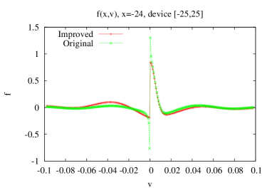
(a) close to the left of the contact

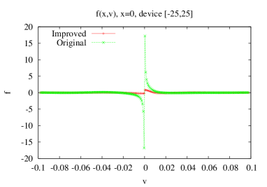
(b) at the center of the device

Figure 1: Device $x\in[-25,25]$. The height of the barrier$H$ is $0.2$, and the barrier is put in the center of devices, $[-1.5,1.5]$. Inflow only from the left contact, $f_{L}(v)=\exp(-v^{2}/0.0002)$ and $f_{R}(v)=0$. $N_{x}=100$. $N_{v}=128$. $R^{h}=2048$. $Ly=31$. $\Delta y=0.5$.

4.2 Convergence

Now we concentrate on studying the convergence with respect to the $x$-mesh size $\Delta x$ and with the $v$-mesh size $\Delta v$, respectively. In this example, we set $f_{L}(v)=e^{-(v-0.5\pi)^{2}/0.25}$, $f_{R}(v)=0$ as the inflow boundary conditions.

To study the convergence of $v$-direction, we fix $N_{x}=100$ ( which corresponds to $\Delta x=0.5$). We fix the velocity interval $[-\pi,\pi]$, and set $\Delta v=\frac{2\pi}{N_{v}}$. The number of velocity points $N_{v}=64,128,256,512,1024$ will be used. Correspondingly, we choose $R^{h}=32,64,128,256,512$, which means $\Delta v$ is equal to $2\pi h$ ($h=\frac{1}{2R^{h}}$). $\Delta y=1.0$ will be used to evaluate the numerical Wigner potential.

The $L_{2}$-norm error is given in the Table 1 where the reference is the solution of the finest mesh ($N_{v}=1024$).

$N_{v}$	Original	Order	Improved	Order
64	0.2756		0.05906
128	0.2466	0.1604	0.01446	2.0301
256	0.2090	0.2386	0.003473	2.0577
512	0.1505	0.4742	0.0007513	2.2090

Table 1: The $L^{2}$-norm error of the distribution function obtained by using the original scheme and the improved scheme with different numbers of velocity mesh points in the fixed velocity interval $[-\pi,\pi]$.

To study the convergence of $x$-direction, we fix the range of velocity $[-\pi,\pi]$, $N_{v}=256$, $R^{h}=128$, $L_{y}=64$. $\Delta y=1.0$. Then we implement the numerical computation by using the orignal scheme and the improved scheme with $N_{x}=25,50,100,200,400$, respectively. We use the numerical distribution calculated on the finnnest mesh $N_{x}=400$ as the reference, then the $L^{2}$-errors and the convergence orders are shown in Table 2.

$N_{x}$	Original	Order	Improved	Order
25	0.4208		0.1653
50	0.1792	1.2322	0.0613	1.4312
100	0.0623	1.5238	0.0156	1.9753
200	0.0131	2.2549	0.0030	2.3590

Table 2: The $L^{2}$-norm error of the distribution function obtained by using the original scheme and the improved scheme with different numbers of $x$ mesh points in the fixed space interval $[-25,25]$.

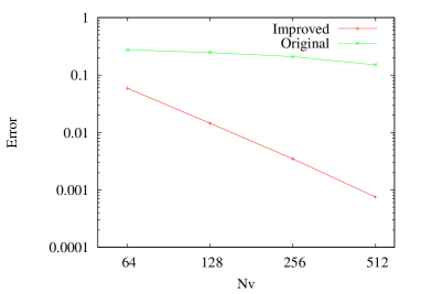
(a) $N_{v}-Error$

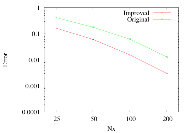
(b) $N_{x}-Error$

Figure 2: Error change with mesh size in $v$-space and $x$-space

We can conclude from Figure 2 that improved scheme converges faster than original scheme in the $v$-direction, which is mainly contributed to the improved scheme is based on the equivalent singularity-free Wigner equation. The convergence order of improved scheme is 2.0948 while that of original scheme is 0.2853 in $v$-space. Original scheme hardly converges for this problem. $x$-direction, original scheme and improved scheme both gain convergence. The convergence order of the original scheme and improved scheme is 1.6556 and 1.9272 respectively. This is roughly conformed to the the theoretical analysis of second-order upwind scheme. Therefore, improved scheme is better than original scheme in convergence.

When we derive the equivalent from of the Wigner equation. We have used an algebra constraint $\eqref{eq:V0}$. In order to check how well the constraint is sastisfied numerically, we introduce

$$S(N_{v})=\max_{i}\left\{\sum_{j=-N_{v}/2}^{N_{v}/2-1}f(x_{i},v_{j})V_{w}(x_{i},v_{j})\Delta v\right\}$$ (52)

which is a numerical approximation of $\max_{x\in[-25,25]}|\int_{\mathbb{R}}V_{w}(x,-v^{\prime})f(x,v^{\prime})\,\mathrm{d}v^{\prime}|$. In Table 3, we list $S(N_{v})$ calculated with different $N_{v}$’s, which shows that $S(N_{v})$ decreases to $0$ with a order $1.0$ as $\Delta v\rightarrow 0$ for both the original scheme and the improved scheme. This implies that the solution of the stationary Wigner equation satisfies the constraction (12), and the explicit use of this property in our improved scheme helps in removing singularity and improving numerical convergence.

$N_{v}$	64	128	256	512	1024
Original	4.7370e-4	2.3550e-4	1.1710e-4	5.8227e-5	2.8945e-5
Improved	4.2746e-4	2.1371e-4	1.0685e-5	5.3427e-5	2.6713e-5

Table 3: $S(N_{v})$ with different $N_{v}$

5 Conclusion

By using an algebra of the stationary Wignner equation, we have proposed a singularity-free scheme, whose numerical convergence with respect to the velocity mesh size has been validated by numerical experiments. We believe that it is the first time that the numerical convergence with respect to the velocity mesh size has been obtained for the stationary Wigner equation with inflow boundary conditions. We will investigate whether it could be applied in simulation of nano-scale semiconductor devices where the potential function may not satisfy the condition in Theorem 1.

References

[1]
A. Arnold, H. Lange, and P.F. Zweifel.
A discrete-velocity, stationary Wigner equation.
J. Math. Phys., 41(11):7167–7180, 2000.
[2]
A. Arnold and C. Ringhofer.
An operator splitting method for the Wigner-Poisson problem.
SIAM Journal on Numerical Analysis, 33(4):pp. 1622–1643, 1996.
[3]
L. Barletti and P. F. Zweifel.
Parity-decomposition method for the stationary Wigner equation with
inflow boundary conditions.
Transport Theory and Statistical Physics, 30(4-6):507–520,
2001.
[4]
B. A. Biegel and J. D. Plummer.
Comparison of self-consistency iteration options for the Wigner
function method of quantum device simulation.
Phys. Rev. B, 54:8070–8082, Sep 1996.
[5]
P. Degond and P.A. Markowich.
A quantum transport model for semiconductors: The
Wigner-Poisson problem on bounded Brillouin zone.
Math. Modell. Numer. Anal., 24:697–709, 1990.
[7]
D.K. Ferry and S.M. Goodnick.
Transport in Nanostructures.
Cambridge Univ. Press, Cambridge, U.K, 1997.
[8]
W.R. Frensley.
Wigner function model of a resonant-tunneling semiconductor device.
Phys. Rev. B, 36:1570–1580, 1987.
[9]
T. Goudon.
Analysis of a semidiscrete version of the Wigner equation.
SIAM J. Numerical Analysis, 40(6):2007–2025, 2003.
[10]
T. Goudon and S. Lohrengel.
On a discrete model for quantum transport in semi-conductor devices.
Transp. Theory Stat. Phys., 31(4-6):471–490, 2002.
[11]
K. L. Jensen and F. A. Buot.
Numerical simulation of intrinsic bistability and high-frequency
current oscillations in resonant tunneling structures.
Phys. Rev. Lett., 66:1078–1081, Feb 1991.
[12]
K.L. Jensen and F.A. Buot.
Numerical aspects on the simulation of I‐V characteristics and
switching times of resonant tunneling diodes.
J. Appl. Phys., 67:2153–2155, 1990.
[13]
H. Jiang, W. Cai, and R. Tsu.
Accuracy of the frensley inflow boundary condition for Wigner
equations in simulating resonant tunneling diodes.
J. Comput. Phys., 230:2031–2044, 2011.
[14]
Kyoung-Youm Kim and Byoungho Lee.
On the high order numerical calculation schemes for the Wigner
transport equation.
Solid-State Electronics, 43(12):2243 – 2245, 1999.
[15]
H. Kosina and M. Nedjalkov.
Wigner function-based device modeling.
In M. Rieth and W. Schommers, editors, Nanodevice Modeling and
Nanoelectronics, volume 10 of Handbook of Theoretical and Computational
Nanotechnology. American Scientific Publishers, 2006.
[16]
R. Li, T. Lu, and Z.-P. Sun.
Stationary wigner equation with inflow boundary conditions: Will a
symmetric potential yield a symmetric solution?
SIAM J. Appl. Math., 70(3):885–897, 2014.
[17]
C. Manzini and L. Barletti.
An analysis of the Wigner-Poisson problem with inflow boundary
conditions.
Nonlinear Analysis, 60:77–100, 2005.
[18]
P.A. Markowich and C. Ringhofer.
An analysis of the quantum liouville equation.
Z. angew. Math. Mech., 69:121–127, 1989.
[19]
O. Morandi.
Quantum corrected Liouville model: mathematical analysis.
J. Math. Phys., 53:063302, 2012.
[20]
M. Nedialkov, H. Kosina, S. Selberherr, C. Ringhofer, and D. K. Ferry.
Unified particle approach to wigner-boltzmann transport in small
semiconductor devices.
Physical Review B, page 115319, 2004.
[21]
H. Neunzert.
The nuclear Vlasov equation: methods and results that can(not) be
taken over from the classical case.
Il Nuovo Cimento, 87A:151–161, 1985.
[22]
C. Ringhofer.
A spectral method for the numerical solution of quantum tunneling
phenomena.
SIAM J. Num. Anal., 27:32–50, 1990.
[23]
J.M. Sellier and I. Dimov.
The wigner–boltzmann monte carlo method applied to electron
transport in the presence of a single dopant.
Computer Physics Communications, 185(10):2427–2435, 2014.
[24]
S. Shao, T. Lu, and W. Cai.
Adaptive conservative cell average spectral element methods for
transient Wigner equation in quantum transport.
Commun. Comput. Phys., 9:711–739, 2011.
[25]
E. Wigner.
On the quantum correction for thermodynamic equilibrium.
Phys. Rev., 40(5):749–759, Jun 1932.
[27]
P.J. Zhao, D.L. Woolard, and H.L. Cui.
Multisubband theory for the origination of intrinsic oscillations
within double-barrier quantum well systems.
Phys. Rev. B, 67:085312, Feb 2003.