Doing Moore with Less – Leapfrogging Moore’s Law with Inexactness for Supercomputing

Abstract

Energy and power consumption are major limitations to continued scaling of computing systems. Inexactness, where the quality of the solution can be traded for energy savings, has been proposed as an approach to overcoming those limitations. In the past, however, inexactness necessitated the need for highly customized or specialized hardware. The current evolution of commercial off-the-shelf (cots) processors facilitates the use of lower-precision arithmetic in ways that reduce energy consumption. We study these new opportunities in this paper, using the example of an inexact Newton algorithm for solving nonlinear equations. Moreover, we have begun developing a set of techniques we call reinvestment that, paradoxically, use reduced precision to improve the quality of the computed result: They do so by reinvesting the energy saved by reduced precision.

We consider the use of low-precision arithmetic in an inexact Newton method to investigate the potential power savings and reinvestment strategies.

The performance of leading supercomputers has increased by an order of magnitude every 3–4 years in the past two decades. The main factors contributing to this growth have been (i) the sustained exponential increase in the performance of processors, as exemplified by Moore’s Law; (ii) a growth in the size of the largest supercomputers and of their energy consumption; and (iii) the use of increasingly specialized and more energy-efficient components, such as GPUs, long vector units, and multicores.

Two of these three factors are running out of steam. Moore’s law is is coming to an end as it has become increasingly difficult, and hence expensive, to reduce the energy consumption of transistors. As devices approach atomic scales, further scaling will require a different technology. There are few alternative technologies that hold a promise of a better energy$\times$delay product and none are close to commercial deployment. Current top supercomputers require power in the range of 10–20MW; it is hard to significantly increase these numbers, because of the cost of energy and the limitation of existing installations. Increased specialization may help, but also leads to increased development costs for the platforms and the application codes using them. Continued increase in effective supercomputer performance will increasingly depend on a smarter use of existing systems, rather than on a brute force increase in their physical performance.

Current supercomputers suffer from the high cost of energy required to run them. Moreover, projected exascale machines will see their costs multiplied by a factor of 1000. Clearly, then, energy-efficient computing techniques are now, and will be, extremely important. Traditionally, users evaluate their computing results with a quality metric. For example, weather prediction focuses heavily on accuracy of weather prediction. Currently, any user seeking improved quality might employ a higher class of supercomputer, bearing the associated energy costs of the higher class of machine. In contrast to this traditional approach, we introduce new techniques that enable a higher quality answer without paying the increased energy costs of a higher-performing CPU. In essence, smart use of a current machine has leapfrogged a machine generation.

Top500 [1], the most commonly cited ranking of supercomputers, measures supercomputer performance by using the number of floating-point operations per second performed in course of solving an as-large-as-feasible, dense system of linear equations (Linpack). A common (and correct) critique of this metric is that the benchmark used is not representative of modern applications. A subtler critique is that the notion of a problem having a unique solution is not representative of modern practice, either. Many modern computational problems have an implicit quality metric, such as precision level. The right question is not how much time or energy it takes to solve a problem; rather it is about the tradeoff between computation and solution quality. Two specific questions naturally arise:

1. What quality of answer can be achieved with a given computation budget (for time or energy)?

2. How large a budget is needed to achieve a certain quality threshold?

Previous research has focused on the second question, and has focused on the compute time budget. We focus on the first question and focus on the energy budget. We believe this novel focus best matches the reality of high-performance computing (HPC): Users attempt to achieve best possible results with a given resource allocation; and the main resource constraint in future systems is energy. This proposed approach can raise the effective performance of systems by focusing attention on the relevant tradeoffs.

To reiterate, ever since energy consumption has become a significant barrier, there has been significant interest in innovative approaches to help continued scaling. In our context, the approach that we build on is the concept of inexact computing[2, 3, 4] which established the principle of trading application quality for disproportionately large energy savings. In this paper, we interpret inexactness to be computational precision.While it is well known that precision reduction can lead to savings, we take the extra step here resulting in a two-phased approach. After applying the traditional inexactness principle during the first phase, we now use a novel second phase which involves reinvesting the saved energy from the first phase, to establish that the quality of the application can be improved significantly, when compared to the original “exact” high-precision computation, all the while using a fixed energy budget.

The study of the precision level of numerical algorithms has been a fundamental subject in numerical analysis since the inception of the field [5, 6]. Much attention has been devoted to the numerical errors induced in simulations by the discretization of continuous space and time; and to the tradeoff between precision level and number of iterations in iterative methods. Less attention has been paid in the HPC world to the discretization of real numbers into 16-, 32-, or 64-bit floating-point values, since the use of lower precision did not result in significant performance gains on commodity processors.

The evolution of technology is changing this balance: Vector operations can perform twice as many single-precision operations as double-precision operations in the same time and using the same energy. Single-precision vector loads and stores can move twice as many words than double precision in the same time and energy budget. The use of shorter words also reduces cache misses. Half precision has the potential to provide a further factor of two. As communication becomes the major source of energy consumption of microprocessors [7, 8], the advantage of shorter words will become more marked. This has led in recent years to a renewed interest in the use of lower-precision arithmetic, where feasible, in HPC [9, 10, 11, 12].

We use the following approach in this paper: We pick as our base computational budget the amount of energy consumed to solve a given problem to a given error bound using double-precision arithmetic. We then examine how that same energy budget can be used to improve the error bound, by using lower-precision arithmetic: We save energy by replacing high precision with lower precision and reinvest these savings in order to improve solution quality.

The organization of the rest of the paper is shown by the following “mini” table of contents:

Application: Solving Nonlinear Equations	This section elaborates the details of our canonical problem — solving nonlinear equations. The method of choice for solving such problems is the inexact Newton’s method.
Experimental Results	This section describes our test machines and experimental methodology. We ran 2 classes of experiments: (1) Simple comparison experiments to determine energy costs of various configurations; and (2) Reinvestment experiments to determine the effectiveness of the reinvestment technique.
The Mathematics of Energy Reinvestment	This section gives a mathematical account of how reinvestment works when viewed through the lens of convergence rates.
Conclusions and Outlook	The final section distills our results into a set of conclusions, and points the way towards broader application of our techniques.

Application: Iteratively Solving Nonlinear Equations

We investigate the effect of low-precision arithmetic on an inexact Newton method. The inexact Newton method [13] considered here, and Jacobian-free Newton-Krylov methods [14] in general, are workhorses in modern nonlinear solvers and provide insight into how low-precision arithmetic can be exploited in scientific computing. Our goal is to solve the nonlinear system of equations

$$F(x)=0,$$ (1)

where $F:\mathbb{R}^{n}\to\mathbb{R}^{n}$ is a twice continuously differentiable function.

The basic inexact Newton method is described in Algorithm 1. It starts from an initial iterate $x^{0}$, and consists of outer and inner iterations. The outer iterations correspond to approximate Newton steps that produce a sequence $\{x^{k}\}_{k}$ of iterates. Given $x^{k}$, the inner iteration solves the Newton system

$$\nabla F(x^{k})s=-F(x^{k})$$ (2)

approximately for $s\in\mathbb{R}^{n}$; in our case, this is done by using BI-CGSTAB [15], but the specific form of inner solver is not a critical part of the present analysis. The inner iterations terminate on the accuracy of the putative direction $s$; that is, one stops when $s$ satisfies a relative residual criterion for (2),

$$\frac{\|\nabla F(x^{k})s+F(x^{k})\|}{\|F(x^{k})\|}\leq\eta_{k},$$ (3)

where $0\leq\eta_{k}<1$ is a sequence of tolerances that is forced to zero as $k$ increases. The search direction, $s$, obtained in the inner iteration is used in a simple Armijo line search [16] in order to ensure global convergence [17]. We note that this line search can fail if the direction $s^{i}$ computed in the inner iteration is not a descent direction for the residual norm, $\|F(x)\|$. In our experiments, we take this failure as an indication that the precision level was too low, and switch to a higher level of precision. More sophisticated approaches (e.g., based on iterative refinement) may also be possible.

Our implementation is somewhat simplistic in the sense that we assume that there exists a solution $x^{*}$ with $F(x^{*})=0$ since we do not implement safeguards that allow convergence to minimizers of the residual $F(x)$ if such a point does not exist. For a more rigorous handling of such cases, see, e.g., [18].

Algorithm 1 Basic Inexact Newton Method.

Input parameters $\eta_{0}>0$, $\epsilon>0$; initialize $x^{0}\in\mathbb{R}^{n}$

Compute $F(x^{0})$ and $\|F(x^{0})\|$; set $k=0$

while $\|F(x^{k})\|>\epsilon$ do

    Approx solve $\nabla F(x^{k})s=-F(x^{k})$ s.t. (3) holds:

    $r^{0}=-F(x^{k})$; set $\|r^{0}\|=\|F(x^{0})\|$

    $q^{0}=r^{0}$, $s^{0}=v^{0}=p^{0}=0$

    $\rho_{0}=\alpha_{0}=\omega_{0}=1$, $i=0$

    while  $\|r^{i}\|>\eta_{k}\|F(x^{k})\|$ do

         $i\leftarrow i+1$

         $\rho_{i}=\mbox{VecVec}\left(q^{0},r^{i-1}\right)$

         if $\rho_{i}=0$ then

             BI-CGSTAB method fails

         end if

         $\beta_{i}=\frac{\rho_{i}}{\rho_{i-1}}\frac{\alpha_{i-1}}{\omega_{i-1}}$

         $p^{i}=r^{i-1}+\beta_{i}(p^{i-1}-\omega_{i-1}v^{i-1})$

         $v^{i}=\mbox{MatVec}\left(\nabla F(x^{k}),p^{i}\right)$

         $\alpha_{i}=\frac{\rho_{i}}{\mbox{VecVec}\left(q^{0},v^{i}\right)}$

         $u^{i}=r^{i-1}-\alpha_{i}v^{i}$

         if $\|u^{i}\|=0$ then

             $s^{i}=s^{i-1}+\alpha_{i}p^{i}$

             exit

         end if

         $t^{i}=\mbox{MatVec}\left(\nabla F(x^{k}),u^{i}\right)$

         $\omega_{i}=\frac{\mbox{VecVec}\left(t^{i},u^{i}\right)}{\mbox{VecVec}\left(t^{i},t^{i}\right)}$

         $s^{i}=s^{i-1}+\alpha_{i}p^{i}+\omega_{i}u^{i}$

         $r^{i}=u^{i}-\omega_{i}t^{i}$; compute $\|r^{i}\|$

    end while

    $\delta=$ LineSearch$(x^{k},s^{i})$ along last $s^{i}$ from inner loop

    Set $x^{k+1}=x^{k}+\delta s^{i}$ and compute $F(x^{k+1})$

    Update $\eta_{k+1}=\min\left\{\|F(x^{k+1})\|^{1/2},\frac{1}{2}\right\}$

    Set $k\leftarrow k+1$ and iterate

end while

Our implementation is matrix-free, in that the Jacobian matrix $\nabla F(x)$ is never explicitly evaluated; the user needs only to implement vector products with the Jacobian matrix. The function MatVec$(A,v)$ in Algorithm 1 implements the matrix-vector product $Av$. The function VecVec$(v,w)$ implements the scalar product $v^{T}w$. To illustrate typical benefits of such an approach, we exploit the fact that the Jacobian matrix in our examples is tridiagonal, and thus we only store the nonzero entries in three vectors of size $n$.

We consider two sets of test problems of variable dimension. The first problem, Laplace, is a well-conditioned linear system of equations, derived from a central-difference discretization of the Poisson equation. We note, however, that because we use an inexact Newton solver, the linear system is not solved in a single outer iteration. The second problem, Rosenbrock, is nonlinear and notoriously ill-conditioned, and was chosen to provide a more strenuous test for our low-precision implementation.

Laplace

The first system of equations is given by

$$F_{1}(x) = b_{1}+4x_{1}-x_{2}$$

$$F_{i}(x) = b_{i}-x_{i-1}+4x_{i}-x_{i+1},\qquad i=2,\ldots,n-1$$

$$F_{n}(x) = b_{n}-x_{n-1}+4x_{n},$$

where $b_{1}=1.0$, $b_{i}=-2.0$ for $i=2,\ldots,n-1$, and $b_{n}=4.0$.

-1 Chained Rosenbrock

The second, nonlinear system of equations is derived from the chained Rosenbrock function

$$\sum_{i=1}^{n-1}\left(a(1-x_{i})^{2}+100\left(x_{i+1}-x_{i}^{2}\right)^{2}\right),$$ (4)

whose first-order optimality conditions provide our system of equations and are given by

$$F_{1}(x) = 2a(x_{1}-1)-400x_{i}\left(x_{2}-x_{1}^{2}\right)$$

$$F_{i}(x) = 200\left(x_{i}-x_{i-1}^{2}\right)+2a(x_{i}-1)$$

$$-400x_{i}\left(x_{i+1}-x_{i}^{2}\right),\qquad i=2,\ldots,n-1$$

$$F_{n}(x) = 200\left(x_{n}-x_{n-1}^{2}\right).$$

The parameter $a>0$ controls the conditioning of the problem; in our tests we use its standard value $a=1$.

Experimental Results

We now describe our experiments with reduced-precision variants of the inexact Newton method.

Experimental Testbed and Analysis Tools

Our hardware testbed for this study was a Dell precision T1700 workstation operated by CentOS 7 and equipped with an Intel core i7 4770 (3.40 GHz) and 16 GB of DDR3 RAM. The processor had 4 cores, each with 2 hyperthreads, giving 8 logical CPUs. The Intel core i7 4770 processor has 2 important architectural features:

1. It implements the AVX2 instructions set

2. It supports the Running Average Power Limit (abbreviated RAPL) hardware counter [19]

Item 2 gives us a way to measure the energy consumption for a given program. The specific RAPL tool that we used, etrace2, was written by one of the authors of this paper.

In order to reduce the noise in our experiments, we launched the same process on all logical CPUs, using Unix taskset to pin each instance of the program being measured to a specific logical CPU. This prevents process migration and avoids background activities on the idle cores. We took the median of 31 separate measurements as our measured energy consumption for a given data point.

The operating system was Linux, kernel 4.3.

We used the Intel compiler IFORT 16.0.3 20160415 to compile our applications. The Intel compiler has exceptional automatic vectorization capabilities.

Experimental Treatments – Configuration Choices

Our experiments were divided into two classes:

Gains.

This suite of experiments was devoted to finding out what gains were possible.

Reinvestment.

Once we had significant energy savings in hand, our next suite of experiments employed our reinvestment technique to improve the quality of our computation.

For both classes of experiment, we employed the inexact Newton algorithm described in Algorithm 1, with the Laplace and Rosenbrock tests problems. We used a problem size of $n=100000$. For each of Laplace and Rosenbrock, in our gains experiments we tested four variants:

1. Scalar arithmetic, double precision

2. Scalar arithmetic, single precision

3. SIMD (vector) arithmetic, double precision

4. SIMD (vector) arithmetic, single precision.

For the reinvestment experiments, we limited our experimentation to the SIMD (vector) configuration, since the vector codes are much more efficient than the scalar ones.

Results of the Gains Experiments

The energy expended by each of the four variants of the Laplace experiment are shown in Fig. 1. The energy expended by each of the four variants on Rosenbrock are shown in Fig. 2.

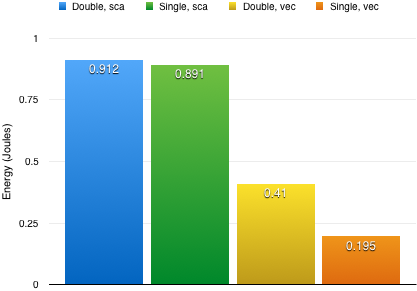
Figure 1: Energy expended by Inexact Newton variants on Laplace; convergence to accuracy $\epsilon=10^{-6}$.

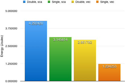
Figure 2: Energy expended by Inexact Newton variants on Rosenbrock; convergence to accuracy $\epsilon=10^{-5}$.

Explaining the Gains

The use of 32-bit (single precision) scalars, rather than 64-bit (double precision) scalars, had limited impact on the energy consumption of arithmetic operations or loads. This is not surprising, since all the data paths, registers and ALUs handle 64-bit values. The use of 32-bit values, has an additional benefit on cache behavior. In general, the beneficial cache effects will depend on the memory access patterns, and how much of the data fits in cache. For the problems we studied in this paper, the data exhibited strong spatial locality — effectively doubling the capacity of caches. This doubling effect greatly reduced the cache misses.

Also, note that vector operations are more energy-efficient, per operand, than scalar operations. Furthermore, a vector arithmetic operation, or a vector load handles twice as many floats as doubles in the same time and energy consumption. Hence, we expect some improvement when moving from vector doubles to vector singles, due to better cache hit ratio significant improvement when going to vector operations, and at least of factor of two improvement when shifting from double vectors to float vectors. The results in Figs. 1 and 2 are consistent with these expectations.

Improving Application Quality Through Reinvestment

Our initial gain experiments show that the SIMD vector codes have better energy savings. Consequently, we now focus on the vectorized variants for our reinvestment experiments.

We recall our reinvestment strategy:

• We run the algorithm in double precision to a given error bound and measure energy consumption. This is our energy budget.

• We next run the algorithm in single precision for a number of iterations, followed by double precision for a number of iterations, consuming the same energy as before, and measure the error bound. The ratio between the first error bound and the second is the achieved improvement factor.

We have not yet developed an algorithm to decide automatically when to switch from single precision to double precision. Therefore, we experiment with different switching points, in order to estimate the gains that reinvestment can achieve.

Our reinvestment experiments have the following steps:

1. Choose a small accuracy tolerance for the single-precision variant. This tolerance is denoted by $\epsilon$ in Algorithm 1.
   Note: A chosen tolerance can result in a line search error, which means that the solution $s^{i}$ of the inner iteration is not a descent direction for the residual norm. We take this failure as an indication that the chosen tolerance is too small.

2. Run the double-precision variant using the same tolerance as step 1.

3. Pick an improvement factor $f$ to try experimentally.

4. Run the reinvestment algorithm in single precision until it achieves the same accuracy tolerance as in step 1; then continue in double precision until this tolerance is further reduced by a factor of $f$. If the energy from this step does not exceed the energy from step 2, then the reinvestment experiment was successful!
   Note:(Again) As in step 1, if a line search error is present in the double-precision reinvestment stage, then the chosen improvement factor is too large.

Laplace

The Laplace example, being linear, quickly converges to a very good approximation of the answer. In our experiments, accuracy tolerance values smaller than $10^{-6}$ resulted in line search errors. These failures are consistent with the fact that $10^{-6}$ is close to single-precision machine precision, so it would be unrealistic to expect better. For Laplace, we were able to achieve an improvement factor of $10^{4}$. The limitation on the improvement factor was the low energy budget. An improvement factor of $10^{5}$ is computationally possible, but the reinvestment energy budget is exceeded for this improvement factor. Improvement factors of $10^{6}$ (or higher) led to line search errors. Details of the experiment appear in Table I; a graphical representation appears in Fig. 3.

TABLE I: Reinvestment for Laplace

Class	Energy	Std	Iterations Single	Iterations Double
	(Joules)	Deviation	Outer/Inner	Outer/Inner
Reinvest	0.843407	0.07	9/12	2/9
Ceiling (double)	1.1026	0.06	NA	8/10
Base (single)	0.510376	0.05	9/12	NA

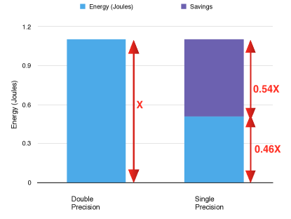
Figure 3: Reinvestment for Laplace; original accuracy $\epsilon=10^{-6}$, improvement factor$=10^{4}$. The “X” graphic shows the total energy budget. The arrows labeled with fractions of “X” show base convergence energy, and energy available for reinvestment.

Rosenbrock

The Rosenbrock example had more scope for experimentation. For our first reinvestment experiment with Rosenbrock, we chose a conservative accuracy tolerance of $10^{-2}$. For this tolerance, both pure single and pure double required 29 (68) outer (inner) iterations. Next, we experimentally determined that $10^{11}$ was the highest improvement factor we could obtain without line search errors in the reinvestment phase. Even with this large improvement factor, we were unable to use all of the saved energy. Table II shows the measured energy and iteration counts; Fig. 4 shows the relative gain savings. Figure 5 shows the fraction of the saved energy that contributed to the reinvestment improvement, as well as the remaining energy.

TABLE II: Reinvestment for Rosenbrock, $10^{-2}$ initial convergence, $10^{11}$ improvement.

Class	Energy	Std	Iterations Single	Iterations Double
	(Joules)	Deviation	Outer/Inner	Outer/Inner
Reinvest	4.20105	0.14	29/68	4/18
Ceiling (double)	6.92410	0.16	NA	29/68
Base (single)	2.69243	0.14	29/68	NA

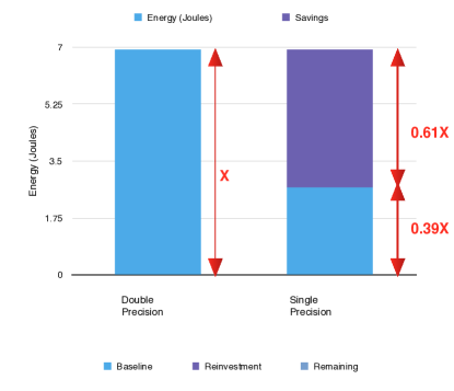
Figure 4: Reinvestment for Rosenbrock; original accuracy $\epsilon=10^{-2}$. The “X” graphic shows the total energy budget. The arrows labeled with fractions of “X” show base convergence energy, and energy available for reinvestment.

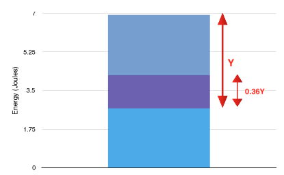
Figure 5: Reinvestment for Rosenbrock; original accuracy $\epsilon=10^{-2}$; $10^{11}$ improvement factor. The “Y” arrow shows the total energy available for reinvestment. The fractional “Y” shows the fraction that could actually be used.

The Rosenbrock example supported a convergence tolerance as small as $10^{-5}$ when using single precision. Smaller tolerances again led to line search errors. In contrast to the Laplace example, convergence on Rosenbrock was slower – 31 outer iterations were required to achieve the desired quality. The large number of iterations, however, meant that there could be substantial savings for reinvestment. We experimentally determined the highest improvement factor to be $10^{8}$; higher factors resulted in line search errors. Even with the high improvement factor, there was still reinvestment energy remaining. Details of the Rosenbrock reinvestment experiment appear in Table III. A single graph showing the baseline, reinvestment, and extra energy can be seen in Fig. 6.

TABLE III: Reinvestment for Rosenbrock, $10^{-5}$ initial convergence, $10^{8}$ improvement.

Class	Energy	Std	Iterations Single	Iterations Double
	(Joules)	Deviation	Outer/Inner	Outer/Inner
Reinvest	4.20730	0.23	31/76	3/14
Ceiling (dbl)	7.84135	0.22	NA	31/76
Base (single)	3.02834	0.31	31/76	NA

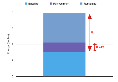
Figure 6: Reinvestment for Rosenbrock; original accuracy $\epsilon=10^{-5}$; improvement factor$=10^{8}$. The “Y” arrow shows the total energy available for reinvestment. The fractional “Y” shows the fraction that could actually be used.

Energy as a Function of Improvement Factor

In the previous section, we were usually working under the assumption that users would seek the largest improvement factor. In reality, a user may seek some improvement, but not the maximum possible improvement. In this section, we show the energy costs of some intermediate improvement factors.

Energy/Improvement Gradations for Laplace

Since the maximum improvement factor for Laplace was $10^{4}$, we looked at improvement factors $10^{1}$, $10^{2}$, $10^{3}$, and $10^{4}$. What we see is that the number of Outer / Inner iterations is the same for each of the improvement factors. This behavior is due to the fact that a single additional outer iteration requires 4 inner iterations, and achieves an improvement factor of $10^{4}$. For Laplace, a user might just as well seek the maximum improvement factor of $10^{4}$.

The table for each of the factors is show in Table IV. Figure 7 shows the same information graphically. Note that the energy numbers are not identical due to measurement error, but lie within the error bounds implied by the standard deviation.

TABLE IV: Energy cost as a function of improvement factor for Laplace; original $\epsilon=10^{-6}$

Improvement	Energy (Joules)	Std	Iterations
Factor (exponent)		Deviation	Outer/Inner
0 (base)	0.510376	0.05	NA/NA
1	0.832625	0.061	1/4
2	0.845	0.053	1/4
3	0.843375	0.056	1/4
4	0.843407	0.07	1/4

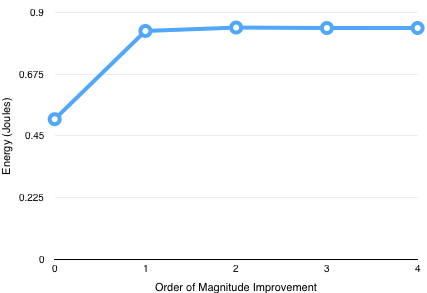
Figure 7: Energy as a function of improvement factor for Laplace; original convergence to accuracy $\epsilon=10^{-6}$.

Energy/Improvement Gradations for Rosenbrock

The Rosenbrock results show 3 clusters of iteration counts: factors 1–2, factors 3–6, and factors 7–8. As with Laplace, these groups correspond to 1, 2, and 3 outer iterations that achieve improvement factors of $10^{2}$, $10^{6}$, and $10^{8}$, respectively. Again, the energy of each group is statistically identical. The details are shown in Table V, with the graphical representation in Fig. 8.

TABLE V: Energy cost as a function of improvement factor for Rosenbrock; original $\epsilon=10^{-5}$

Improvement	Energy (Joules)	Std	Iterations
Factor (exponent)		Deviation	Outer/Inner
0 (base)	3.0283	0.31	NA/NA
1	3.3562	0.158	1/4
2	3.385	0.052	1/4
3	3.7488	0.066	2/8
4	3.7762	0.038	2/8
5	3.7775	0.077	2/8
6	3.7762	0.054	2/8
7	4.2575	0.075	3/14
8	4.2073	0.23	3/14

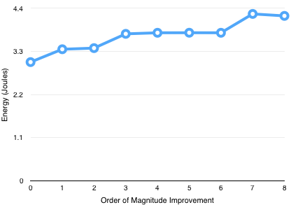
Figure 8: Energy as a function of improvement factor for Rosenbrock; original convergence to accuracy $\epsilon=10^{-5}$.

The Mathematics of Energy Reinvestment

We present a model of the reinvestment of the energy saved using low-precision arithmetic, and show that under fairly mild assumptions, we can expect to obtain a more accurate solution at a reduced cost, and we quantify the potential savings in the example of our inexact Newton applications.

Given its iterative nature and adaptive accuracy requirements, the inexact Newton method lends itself almost ideally to an approach that seeks to take advantage of inexact and adaptive-precision arithmetic. We are motivated by the observation that most of the work of Newton’s method typically occurs before the transition to fast quadratic convergence.

In Algorithm 2, we propose a simple meta-strategy that starts by running Algorithm 1 with low-precision arithmetic, and switches to increasingly higher accuracy levels as we approach the solution. It consists of running the inexact Newton method at prescribed precision levels, with an accuracy tolerance, discussed further below, based on the current precision level. Many other approaches are possible, but this simple meta-strategy facilitates analysis and is representative of other inexactness-switching-based strategies for linear and nonlinear solvers [20, 21].

Algorithm 2 Meta Strategy for Inexact Newton.

Given precision levels $p_{1}<p_{2}<\ldots<p_{L}$.

Initialize $x^{0}\in\mathbb{R}^{n}$.

for $l=1,\ldots,L$ do

    Obtain solution $x^{l}$ by running Algorithm 1 at precision level $p_{l}$ starting from $x^{l-1}$ (to an accuracy level $\epsilon=$Ep$(p_{l},x^{l-1})$ depending on the precision level).

end for

Energy Model for Floating-Point Operations

We generalize the energy model in [22] and derive an energy model for each individual iteration of inexact Newton that also takes cache misses into account. We note that for both equations (Laplace and Rosenbrock) solved by our inexact Newton code have tridiagonal Jacobians. Hence, the MatVec operation for our particular test cases is $O(n)$, rather than $O(n^{2})$ in the dense case. All other operations in any given iteration are also $O(n)$.

We let $kn$ denote the number of floating-point operations at an outer iteration, and $ln$ denote the number of floating-point storage locations. In our examples, both $k$ and $l$ are small integers when compared with the problem dimension $n$. We let $E_{c}(p)$ and $E_{t}(p)$ denote the energy required for a single floating-point compute and transfer, respectively, at precision level p. We neglect the cost of L1 cache transfers, and instead only consider L2 and L3 cache transfers. We let $r(p)$ denote the cache-miss rate at precision level $p$ (i.e., number of bits).

We assume that energy and cache-miss rates scale linearly with the precision-level $p$. For the sake of convenience, we assume that energy and miss-rates can be simply expressed as

$$E_{c}(p)=pE_{c},\quad E_{t}(p)=pE_{t},\quad r(p)=pr.$$ (5)

Under these assumptions, it follows that the energy required for a single outer iteration is

$$E(p)=knE_{c}p+lnrpE_{t}p=knE_{c}p+lnrE_{t}p^{2},$$ (6)

where the second term depends quadratically on the precision, because both the cache-miss rate, $r(p)$, and the transfer energy, $E_{t}(p)$, are linear functions of the precision level. Although this may indicate that we can expect superlinear energy savings, the rate constant is typically too small (in practice, $r$ takes values $r\in[10^{-3},10^{-6}]$), and the linear term dominates.

Model for Reinvestment Strategy

Here, we develop a mathematical model for the reinvestment strategy described in Algorithm 2. Formally, we compare the accuracy of a computation done using double precision to the accuracy of a computation using the same amount of energy, but using single precision, where feasible. The analysis can be extended to the case of more than two levels of precision.

We denote by $\epsilon_{k}=\|F(x^{k})\|$ the error at the $k$th outer iteration and assume, without loss of generality, that $\epsilon_{0}\leq 1$.

We also assume that the method can use a precision of $p$ as long as $\epsilon>2^{-p+s}$. That is, that the inner and outer loops will terminate provided the current solution error is large with respect to the precision of floating-point arithmetic. The $s$ term relates to the length of the exponent, and to the amount of rounding errors accumulated during an outer iteration.

To simplify the discussion, we shall assume that $s=3\lg p-7+\delta$. The value of $2^{-p+3\lg p-7}$ is $2^{-11}$, $2^{-24}$, and $2^{-53}$ for $p=16,32,64$, respectively, and approximates machine epsilon in the IEEE 754 standard (see, e.g., [23]). The $2^{\delta}$ term captures the conditioning of the problem; for simplicity, we use $\delta=8$ here, so that we can use single precision if $\epsilon>2^{-16}\approx 10^{-5}$ and double precision if $\epsilon>2^{-45}\approx 3\cdot 10^{-14}$.

The advantage of lower precision will depend on the rate of convergence of the iterative method.

Models Assuming Linear Convergence

We consider first the case where the iterative method converges linearly: $\epsilon_{k+1}\leq\epsilon_{k}/\lambda$, with $\lambda>1$. Since $\epsilon_{0}\leq 1$, the error after $k$ iterations is bounded by $\epsilon_{k}\leq\lambda^{-k}$, provided that the precision level $p$ satisfies $\epsilon_{k}\geq 2^{-p+s}$. Combining these two bounds, we see that at most $\frac{p-s}{\lg\lambda}$ such iterations are possible.

Now suppose that we have two precision levels, $p_{1}<p_{2}$ and an accuracy level $\epsilon$ that is attainable by the higher-precision level $p_{2}$ (i.e., $\epsilon\geq 2^{-p_{2}+s_{2}}$). The energy consumed by this baseline precision to be guaranteed an accuracy level $\epsilon$ is

$$E(p_{2})\frac{\lg\frac{1}{\epsilon}}{\lg\lambda}.$$ (7)

Now consider a hybrid procedure that performs $k_{1}$ iterations at precision level $p_{1}$ followed by $k_{2}$ iterations at precision level $p_{2}$. The energy consumed by such a hybrid procedure is

$$E(p_{2})\left(k_{1}\frac{E(p_{1})}{E(p_{2})}+k_{2}\right).$$ (8)

If we require that the energy consumed by the hybrid procedure is no more than that for the baseline ($p_{2}$) procedure, then (7) and (8) imply that we must have the following bound on the number of iterations at the higher-precision level:

$$k_{2}\leq\frac{\lg\frac{1}{\epsilon}}{\lg\lambda}-k_{1}\frac{E(p_{1})}{E(p_{2})}.$$ (9)

Applying (9), we have that the accuracy of the hybrid procedure is therefore bounded by

$$\epsilon_{k_{1}+k_{2}}\leq\lambda^{-k_{1}-k_{2}}\leq\lambda^{-k_{1}\left(1-\frac{E(p_{1})}{E(p_{2})}\right)-\frac{\lg\frac{1}{\epsilon}}{\lg\lambda}}.$$ (10)

Since $\lambda>1$ and $E(p_{1})<E(p_{2})$, the bound in (10) is decreasing in the number of lower-precision iterations, $k_{1}$, and thus one should choose $k_{1}$ to be as large as possible. The bound in (10), however, only applies if the accuracy level $\lambda^{-k_{1}}$ is attainable at the lower-precision level; that is, if the lower-precision number of iterations satisfies $k_{1}\leq\frac{p_{1}-s_{1}}{\lg\lambda}$. Similarly, the accuracy level $\epsilon_{k_{1}+k_{2}}$ is only attainable at the higher-precision level if $\epsilon_{k_{1}+k_{2}}\geq 2^{-p_{2}+s_{2}}$. Applying these two inequalities to the bound in (10), we have that

$$\begin{array}[]{rl}\epsilon_{k_{1}+k_{2}}&\leq\max\left\{2^{-p_{2}+s_{2}},\lambda^{-\frac{p_{1}-s_{1}}{\lg\lambda}\left(1-\frac{E(p_{1})}{E(p_{2})}\right)-\frac{\lg\frac{1}{\epsilon}}{\lg\lambda}}\right\}\\ &=\max\left\{2^{-p_{2}+s_{2}},2^{-(p_{1}-s_{1})\left(1-\frac{E(p_{1})}{E(p_{2})}\right)-\lg\frac{1}{\epsilon}}\right\}\\ &=2^{-\min\left\{p_{2}-s_{2},(p_{1}-s_{1})\left(1-\frac{E(p_{1})}{E(p_{2})}\right)+\lg\frac{1}{\epsilon}\right\}},\end{array}$$ (11)

where the first equality follows from the relation $\lambda^{\frac{b}{\lg\lambda}}=2^{b}$.

The improvement factor thus satisfies

$$\frac{\epsilon}{\epsilon_{k_{1}+k_{2}}}\geq 2^{\min\left\{\lg\epsilon+p_{2}-s_{2},(p_{1}-s_{1})\left(1-\frac{E(p_{1})}{E(p_{2})}\right)\right\}}.$$ (12)

We note that this bound relates the improvement factor to the original accuracy ($\epsilon$), the precision levels ($p_{i}-s_{i}$), and the energy ratio ($\frac{E(p_{1})}{E(p_{2})}$). Figure 9 illustrates this bound for a variety of precision levels under the assumptions $s_{i}=3\lg p_{i}+1$ and $\frac{E(p_{1})}{E(p_{2})}=\frac{p_{1}}{p_{2}}$.

We also note that these bounds are not necessarily tight, and thus even larger improvement factors can be seen in practice. As a specific example, for the hybrid Rosenbrock measurements in Table III with $\frac{E(p_{1})}{E(p_{2})}\approx 0.3$, then $p_{1}=32$, $s_{1}=s_{2}=0$, and (12) give the bound $\frac{\epsilon}{\epsilon_{k_{1}+k_{2}}}\geq 5.5\cdot 10^{6}$. This bound is still more than an order of magnitude short of the measured improvement factor $10^{8}$.

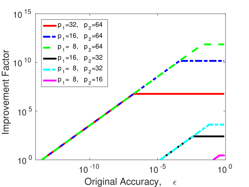
Figure 9: Improvement factor bound (12) for linear convergence rate as a function of $\epsilon$ for different hybrid precision levels (assumes $s_{i}=3\lg p_{i}+1$ and $\frac{E(p_{1})}{E(p_{2})}=\frac{p_{1}}{p_{2}}$).

Neglecting the reinvestment strategy for the moment, we also examine the energy expended for generic hybrid schemes. By using the optimal value $k_{1}=\frac{1}{\lg\lambda}\min\left\{p_{1}-s_{1},\lg\frac{1}{\epsilon}\right\}$ and the corresponding

$$k_{2}=\frac{1}{\lg\lambda}\min\left\{p_{2}-s_{2},\max\left\{0,\lg\frac{1}{\epsilon}-k_{1}\lg\lambda\right\}\right\},$$

we can calculate via (8) the energy expended to attain an accuracy $\epsilon$. This is illustrated in Fig. 10 for a variety of precision levels, under the assumptions $s_{i}=p_{i}/2$ and $E(p_{i})\propto p_{i}$.

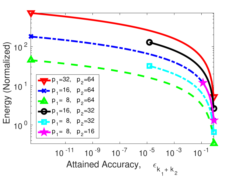
Figure 10: Energy (less a normalizing constant) expended for linear convergence rate as a function of $\epsilon$ for different hybrid precision levels (assumes $s_{i}=3\lg p_{i}+1$ and $E(p)\propto p$).

Quadratic Convergence

For an iterative method with a quadratic convergence rate, one has that $\epsilon_{k+1}\leq(\epsilon_{k})^{2}/\lambda$, where $\lambda>1$. The error after $k$ iterations is thus bounded by $\epsilon_{k}\leq\lambda^{-2k+1}$. In order to satisfy $\epsilon_{k}\geq 2^{-p+s}$, at most $\frac{p-s}{2\lg\lambda}+\frac{1}{2}$ iterations at a precision level $p$ are possible.

Applying similar arguments as in the case of the linear convergence rate, we have that the accuracy of a hybrid, quadratically converging procedure is bounded by

$$\begin{array}[]{rl}\epsilon_{k_{1}+k_{2}}&\leq\max\left\{2^{-p_{2}+s_{2}},\lambda^{-\left(\frac{p_{1}-s_{1}}{\lg\lambda}+1\right)\left(1-\frac{E(p_{1})}{E(p_{2})}\right)-\frac{\lg\frac{1}{\epsilon}}{\lg\lambda}+1}\right\}\\ &=2^{-\min\left\{p_{2}-s_{2},\left(p_{1}-s_{1}\right)\left(1-\frac{E(p_{1})}{E(p_{2})}\right)+\lg\frac{1}{\epsilon}-\frac{E(p_{1})}{E(p_{2})}\lg\lambda\right\}}.\end{array}$$ (13)

Thus, either the higher-precision level’s attainable accuracy is binding, or the achieved accuracy is changed from that in (11) by a modest factor $\lambda 2^{\frac{E(p_{1})}{E(p_{2})}}$. Therefore the improvement factor lower bound decreases by at most a factor $\lambda^{-1}2^{-\frac{E(p_{1})}{E(p_{2})}}$.

Conclusions and Outlook

We have developed in this paper a somewhat paradoxical procedure for reducing the errors in numerical computations by reducing the precision of the floating point operations used. Our focus has been on using in the best possible manner a given energy budget. The paper illustrated one possible tradeoff between computation budget and quality, namely the one achieved by changing numerical precision of floating point numbers. As mentioned in the introduction, there are many other potential “knobs” to trade off quality against computation budget: One can use different approximations in the mathematical model, different computation methods, different discretizations of the continuous model, different levels of asynchrony, etc. Each of these knobs has been studied in isolation. But there are not independent; we are missing a methodology for finding the combination of choices for these knobs that achieve the best tradeoff between quality and computation effort.

The “dual” problem, or reducing energy consumption for a given result quality, is also important. Our results essentially show that one can reduce energy consumption by a factor of $2.x$, without affecting the quality of the result, by smarter use of single precision. For decades, increased supercomputer performance has meant more double precision floating point operations per second. This brute force approach is going to hit a brick wall pretty soon. Smarter use of available computer resources is going to be the main way of increasing the effective performance of supercomputers in the future.

Among the many scientific domains where effective supercomputing has come to play a central role, none are perhaps more important than weather prediction and climate modeling. Inexactness or phase I of our approach has been shown in earlier work [24, 22] to yield benefits to weather prediction models with lower energy consumption while preserving the quality of the prediction. This has spurred interest among climate scientists who view inexactness through precision reduction as a way of achieving speedups in the traditional sense, and also cope with energy barriers [25, 26]. However, it is well understood that for serious advances in model quality, weather and climate models need to be resolved at much higher resolutions that is possible today with current computational budgets including energy. We hope that the new direction that the results in this paper have demonstrated through the novel approach of reinvestment to raising application quality significantly, will be a harbinger for broader adoption of our two-phased approach by the weather and climate modeling community. In particular, building on our work here, the goal of selectively reducing precision resulting in energy savings, while increasing the resolution of the weather and climate models through energy reinvestment provides a path of considerable societal value.

References

- [1] “Top500 supercomputer site,” 2016 [Last accessed 9/27/16], http://www.top500.org.
- [2] K. Palem, “Proof as experiment: Algorithms from a thermodynamic perspective,” in Proceedings of The Intl. Symposium on Verification (Theory and Practice), July 2003.
- [3] S. Cheemalavagu, P. Korkmaz, and K. V. Palem, “Ultra low-energy computing via probabilistic algorithms and devices: CMOS device primitives and the energy-probability relationship,” in Proc. of The 2004 International Conference on Solid State Devices and Materials, 2004, pp. 402–403.
- [4] K. Palem, “Energy aware computing through probabilistic switching: A study of limits,” IEEE Transactions on Computers, vol. 54(9), pp. 1123–1137, September 2005.
- [5] R. W. Hamming, Numerical Methods for Scientists and Engineers (2nd Ed.). New York: Dover Publications, 1986.
- [6] J. H. Wilkinson, Rounding Errors in Algebraic Processes. New York: Dover Publications, 1994.
- [7] K. Bergman, S. Borkar, D. Campbell, W. Carlson, W. Dally, M. Denneau, P. Franzon, W. Harrod, K. Hill, J. Hiller et al., “Exascale computing study: Technology challenges in achieving exascale systems,” Defense Advanced Research Projects Agency Information Processing Techniques Office (DARPA IPTO), Tech. Rep, vol. 15, 2008.
- [8] J. Ang, R. F. Barrett, R. Benner, D. Burke, C. Chan, J. Cook, D. Donofrio, S. D. Hammond, K. S. Hemmert, S. Kelly et al., “Abstract machine models and proxy architectures for exascale computing,” in Hardware-Software Co-Design for High Performance Computing (Co-HPC), 2014. IEEE, 2014, pp. 25–32.
- [9] A. Buttari, J. Dongarra, J. Langou, J. Langou, P. Luszczek, and J. Kurzak, “Mixed precision iterative refinement techniques for the solution of dense linear systems,” International Journal of High Performance Computing Applications, vol. 21, no. 4, pp. 457–466, 2007.
- [10] M. Baboulin, A. Buttari, J. Dongarra, J. Kurzak, J. Langou, J. Langou, P. Luszczek, and S. Tomov, “Accelerating scientific computations with mixed precision algorithms,” Computer Physics Communications, vol. 180, no. 12, pp. 2526–2533, 2009.
- [11] X. S. Li, J. W. Demmel, D. H. Bailey, G. Henry, Y. Hida, J. Iskandar, W. Kahan, S. Y. Kang, A. Kapur, M. C. Martin, B. J. Thompson, T. Tung, and D. J. Yoo, “Design, implementation and testing of extended and mixed precision BLAS,” ACM Transactions on Mathematical Software, vol. 28, no. 2, pp. 152–205, Jun. 2002.
- [12] C. Rubio-González, C. Nguyen, H. D. Nguyen, J. Demmel, W. Kahan, K. Sen, D. H. Bailey, C. Iancu, and D. Hough, “Precimonious: Tuning assistant for floating-point precision,” in Proceedings of the International Conference on High Performance Computing, Networking, Storage and Analysis, ser. SC ’13. ACM, 2013, pp. 27:1–27:12.
- [13] R. S. Dembo, S. C. Eisenstat, and T. Steihaug, “Inexact Newton methods,” SIAM Journal on Numerical Analysis, vol. 19, no. 2, pp. 400–408, 1982.
- [14] D. A. Knoll and D. E. Keyes, “Jacobian-free Newton-Krylov methods: A survey of approaches and applications,” Journal of Computational Physics, vol. 193, no. 2, pp. 357–397, 2004.
- [15] H. A. van der Vorst, “Bi-CGSTAB: a fast and smoothly converging variant of Bi-CG for the solution of nonsymmetric linear systems,” SIAM Journal on Scientific and Statistical Computing, vol. 13, no. 2, pp. 631–644, 1992.
- [16] L. Armijo, “Minimization of functions having Lipschitz continuous first partial derivatives,” Pacific Journal of Mathematics, vol. 16, no. 1, pp. 1–3, 1966.
- [17] C. T. Kelley, Solving Nonlinear Equations with Newton’s Method. Philadelphia: SIAM, 2003.
- [18] N. I. M. Gould, S. Leyffer, and P. L. Toint, “A multidimensional filter algorithm for nonlinear equations and nonlinear least-squares,” SIAM Journal on Optimization, vol. 15, no. 1, pp. 17–38, 2004.
- [19] H. David, E. Gorbatov, U. R. Hanebutte, R. Khanna, and C. Le, “RAPL: memory power estimation and capping,” in 16th ACM/IEEE International Symposium on Low Power Electronics and Design, ser. ISLPED ’10, 2010, pp. 189–194.
- [20] P. D. Hovland and L. C. McInnes, “Parallel simulation of compressible flow using automatic differentiation and PETSc,” Parallel Computing, vol. 27, no. 4, pp. 503–519, 2001.
- [21] G. H. Golub and Q. Ye, “Inexact preconditioned conjugate gradient method with inner-outer iteration,” SIAM Journal on Scientific Computing, vol. 21, no. 4, pp. 1305–1320, 1999.
- [22] P. Düben, J. Schlachter, Parishkrati, S. Yenugula, J. Augustine, C. Enz, K. Palem, and T. N. Palmer, “Opportunities for energy efficient computing: A study of inexact general purpose processors for high-performance and big-data applications,” in Proceedings of the 2015 Design, Automation & Test in Europe Conference & Exhibition (DATE ’15), 2015, pp. 764–769.
- [23] J. W. Demmel, Applied Numerical Linear Algebra. Philadelphia: SIAM, 1997.
- [24] P. D. Düben, J. Joven, A. Lingamneni, H. McNamara, G. De Micheli, K. V. Palem, and T. Palmer, “On the use of inexact, pruned hardware in atmospheric modeling,” Philosophical Transactions of the Royal Society of London A: Mathematical, Physical and Engineering Sciences, vol. 372, no. 2018, p. 20130276, 2014.
- [25] T. Palmer, “Modelling: Build imprecise supercomputers,” Nature, September 29 2015.
- [26] P. Bauer, A. Thorpe, and G. Brunet, “The quiet revolution of numerical weather prediction,” Nature, pp. 47–55, September 15 2015.