Exploring brain transcriptomic patterns: a topological analysis using spatial expression networks

Abstract

Characterizing the transcriptome architecture of the human brain is fundamental in gaining an understanding of brain function and disease. A number of recent studies have investigated patterns of brain gene expression obtained from an extensive anatomical coverage across the entire human brain using experimental data generated by the Allen Human Brain Atlas (AHBA) project. In this paper, we propose a new representation of a gene’s transcription activity that explicitly captures the pattern of spatial co-expression across different anatomical brain regions. For each gene, we define a Spatial Expression Network (SEN), a network quantifying co-expression patterns amongst several anatomical locations. Network similarity measures are then employed to quantify the topological resemblance between pairs of SENs and identify naturally occurring clusters. Using network-theoretical measures, three large clusters have been detected featuring distinct topological properties. We then evaluate whether topological diversity of the SENs reflects significant differences in biological function through a gene ontology analysis. We report on evidence suggesting that one of the three SEN clusters consists of genes specifically involved in the nervous system, including genes related to brain disorders, while the remaining two clusters are representative of immunity, transcription and translation. These findings are consistent with previous studies showing that brain gene clusters are generally associated with one of these three major biological processes.

I Introduction

The human brain is a complex interconnected structure controlling all elementary and high-level cognitive tasks [1]. This complexity is a result of the cellular diversity distributed across hundreds of distinct brain anatomical structures [2, 3]. One of the main tasks of the neuroscience community in the past decade has been to connect the underlying genetic information of the anatomical structures to their underlying biological function [3, 4, 5]. A useful data source for such studies is the Allen Human Brain Atlas (AHBA) [3], which provides microarray expression profiles of almost every gene of the human genome with emphasis on an extensive anatomical coverage across the entire human brain.

In this paper, we make use of the experimental data provided by the AHBA project to study the spatial microarray variability at the single gene level. Analyzing the complete transcription architecture of the human brain in this way may be informative of the impact of genetic disorders on different brain regions that would otherwise not be apparent due to the coarse resolution.

To gain new insights into the expression patterns of the human brain and identify potentially important biomarkers, many studies involving the AHBA data explore gene to gene relationships [3, 4]. Each gene is represented by its expression levels across anatomical locations. Genes with correlated expression profiles are grouped together based on an appropriate similarity measure. The analysis of the resulting gene co-expression networks provides evidence that transcriptional regulation relates to anatomy and brain function [2, 3, 4]. There are also studies that consider the genetic similarity between pairs of regions, and show that transcriptional regulation varies enormously with anatomic location [3, 4, 6, 7]. These findings indicate the necessity to adopt a new representation of a gene’s transcription activity that explicitly captures the pattern of spatial co-expression across different anatomical brain regions.

We propose a new and unexplored way to model the spatial variability at the single gene level. For each gene, we create a spatial expression network, or SEN. Each node of the network corresponds to a pre-defined brain region for which we have sufficient transcriptomic data, and each edge weight represents the similarity in gene expression levels, for that gene, between two brain regions. Applying this procedure to genes that have been found to be stably expressed across specimens gives rise to a population of approximately $17,000$ gene networks, each one representing a brain-wide spatial pattern of gene expression. Using this representation, we investigate whether the topological similarity of the SENs reflects the biological similarity of genes through an integrative analysis based on network clustering and gene ontologies. Our hypothesis is that, if clusters of topologically similar SENs can be identified, the corresponding genes within each cluster may also share similar biological properties.

Figure 1: Anatomical maps of the $105$ brain regions used to construct the SENs. The maps show the brain regions as seen from inferior, lateral and superior views, from left to right. All regions are in the left hemisphere and they are located in the Thalamus, Cerebellum, Pons, Midbrain, Medulla and Cerebral cortex. Coloring of the regions is consistent with anatomical tissue and is obtained from AHBA ontology atlas [8].

A robust cluster analysis of all SENs has indicated the presence of three large and stable clusters of SENs, each one having significantly different topological features as well as different biological function. In particular, one of the clusters has been found to be uniquely enriched for brain-related terms, neurological diseases and genes with enriched expression in neurons. Overall, our analysis provides evidence supporting the notion that topological proximity of spatial gene networks is indicative of similar biological function.

II Materials and Methods

II-A Spatial Expression Networks (SENs)

The Allen Human Brain Atlas (AHBA) [8, 3] is a publicly available atlas of the human brain with microarray-based genome-wide transcriptional profiling of specific brain regions spanning all major anatomical structures of the adult brain. The data set includes transcriptional profiling data from more than $3500$ samples comprising approximately $200$ brain regions in $6$ clinically unremarkable adult human brains. The Agilent $4\times 44$ Whole Human Genome platform was used for gene expression extraction. Two donors contributed samples representing approximately $1000$ structures across the whole brain, while the other four approximately $500$ samples from the left hemisphere. Our analyses is based on $16,906$ pre-selected genes from a previous study [5]. We use the normalized expression levels, which were normalized across samples and across different brains as in previous analyses [9].

For each of the $16,906$ genes, we constructed an individual spatial expression network (SEN) representing patterns of expression variability in the brain. Only brain regions with at least one measurement in all $6$ brains were included in the analysis resulting in a total of $N=105$ regions from the left hemisphere, as shown in Fig. 1.

The mean expression level for a gene in brain region $i$ is denoted by $g_{i}$. The distribution of the mean and median values for each brain region over all genes were not found statistically different (Kolmogorov-Smirnov test [10]; all $p>>0.05$). Furthermore, for more than $97\%$ of all region samples across all genes, the standard deviation of the expression values is less than $20\%$ of the mean value, indicating that the mean can be taken as representative of the expression values at a given region for a given gene.

Formally, we define a SEN as a fully connected network $G=(V,E)$ with node set $V=\{i:i=1,2,...,N\}$ indicating the brain regions and weighted edge set $E=\{E_{ij}:i,j=1,2,...,N;i\neq j\}$. Each edge weight $E_{ij}\in[0,1]$ quantifies the similarity in gene expression between regions $i$ and $j$. The maximum value is reached when the mean expression levels in the two brain regions are equal. We impose that $E_{ij}$ monotonically decreases with an increasing absolute difference between mean expression levels; accordingly, the edge weights are defined as

$$E_{ij}:=\frac{1}{1+|g_{i}-g_{j}|}.$$

This network representation allows us to capture the interconnected variability of gene expression across the brain at the gene level.

II-B Clustering SENs

In order to address our hypothesis that topological similarity may reflect biological similarity, initially we set out to explore whether SENs form naturally occurring clusters. For this we first required an appropriate measure of topological dissimilarity between pairs of SENs. We first mapped each SEN $G$ to a $N$-dimensional feature vector $\bm{d}=\left(d_{1},d_{2},...,d_{N}\right)$ with each elements representing the node degree, i.e. $d_{i}=\sum_{j=1}^{N}E_{i,j}$. The degree for each node captures the global transcriptomic similarity of the corresponding brain region to all other brain regions for a given gene. If the node degrees for two SENs are very different, then the corresponding genes have very different global transcriptomic patterns. The dissimilarity between two SENs, $G_{l}$ and $G_{k}$, was taken to be the Euclidean distance between the corresponding feature vectors, $\bm{d}_{l}$ and $\bm{d}_{k}$.

Three different clustering algorithms were used – partitioning around medoids (PAM) [11], k-means [12] and fuzzy C-means [13] – all providing a partition of all the SENs into $k$ different clusters. To determine an appropriate number of clusters $k$ using each one of these algorithms we performed a stability analysis [12]. The $k$ clusters are deemed “stable” if random changes in the SEN configurations generate almost identical $k$ clusters. To introduce random changes in the networks, we use a randomization strategy by which the observed networks in network space $\Gamma$ are perturbed slightly. For this analysis we used two different randomization procedures: (a) vertex permutations, i.e. we permuted the node labels of a random subset of networks so as to preserve the node degrees but not their order, (b) edge perturbation, i.e. we perturbed the edge weights of a random subset of networks so as to make the cluster robust against white noise.

To obtain a measure of cluster instability, we use the following steps: First, we generate perturbed versions $\Gamma_{b}\left(b=1,2,...,b_{\max}\right)$ of $\Gamma$, and cluster the networks in $\Gamma_{b}$ into $k$ clusters thus obtaining $\mathcal{C}_{b}(k)$. In addition, we randomize the cluster assignments [14] in $\mathcal{C}_{b}\left(k\right)$ to obtain random clustering $\mathcal{C}_{b,\text{rand}}\left(k\right).$ Second, for $b,b^{\prime}=1,2,...,b_{\max}$, we compute the pairwise distances $\left[1-NMI(\mathcal{C}_{b}(k),\mathcal{C}_{b^{\prime}}(k))\right]$ between the clusterings $\mathcal{C}_{b}(k)$ and $\mathcal{C}_{b^{\prime}}(k),$ and between the randomized clusterings $\mathcal{C}_{b,\text{rand}}(k)$ and $\mathcal{C}_{b^{\prime},\text{rand}}(k)$. The normalized mutual information (NMI) is used as a similarity measure between partitions [15]. The cluster instability index is defined as the mean distance between clusterings $\mathcal{C}_{b}(k)$, i.e.

$$I(k)=\frac{1}{b_{\max}^{2}}\sum_{b,b^{\prime}=1}^{b_{\max}}\left[1-NMI(\mathcal{C}_{b}(k),\mathcal{C}_{b^{\prime}}(k))\right].$$ (1)

We use the normalized instability index, $I_{\text{norm}}(k):=I(k)/I_{\text{rand}}(k)$, which corrects for a scaling [14] of $I(k)$ with an increasing number of clusters $k$. We choose number of clusters $k$ that gives the lowest $I_{\text{norm}}(k).$

II-C Topological characterization of SEN clusters

To characterize the topological properties of SENs in each cluster, we use global topological measures that capture different aspect of the network such as its density, the tendency of its nodes to cluster and form communities, the presence of central and hub nodes. Overall, we use eight such different measures: average node degree [16], average closeness centrality [16], weighted diameter [17], global clustering coefficient for weighted networks [17], number of non-overlapping communities, average authority score [18], the number of nodes with authority score $>0.95$, and the number of nodes with authority score $<0.05$. All measures were computed for all SENs within each cluster. To test for statistically significant differences in network topology across clusters, we performed a multivariate ANOVA test [19].

Furthermore, for each SEN we derived a measure of community structure [20]. In our context, the presence of a community in a given SEN indicates that there is a set of highly interconnected brain regions whose gene expression similarity is higher compared to the rest of the network. For this analysis we used the Fast Greedy algorithm [21], which is based on the optimization of the modularity function that sums the edge weights within a community and corrects for the expected edge weights by chance. The algorithm is discriminative of small edge weight differences and can yield sensitive separation of brain regions into communities. Genes with similar community structures indicate the presence of similar local coherent transcriptomic patterns for groups of brain regions.

For each cluster, we quantify the similarity of a pair of brain regions using the communities detected in all the SENs by counting the number of times the two regions fall within the same community. This count is then divided by the total number of SENs in the cluster in order to obtain an index lying in the $[0,1]$ range, which we call the “coherence index”. Values close to $1$ indicate high coherency between the two brain regions, i.e. the average tendency to fall within communities of highly interconnected brain regions.

II-D Biological characterization of SEN clusters

In order to investigate whether naturally occurring clusters formed by SENs can be related to distinct biological function, we require a procedure which assigns representative biological terms to each cluster. For this purpose we use a Gene Ontology (GO) enrichment analysis pipeline which first collects broad GO information for the biological context of genes in each of the main clusters, and then reduces this information to representative GO terms for final interpretation of the clusters.

Each SEN cluster was first annotated for significantly enriched Biological Process (BP) terms using a standard hypergeometric test for over-represented terms ($p<0.001$) implemented in the GOstats R package [22]. Using a clustering methodology implemented in the tool REVIGO [23], we group semantically similar GO terms based on the established SimRel measure. The algorithm finds a representative term for each group based on the enrichment p-values, with a bias away from very general parent GO terms. The size of the resulting summary list is controlled by setting the threshold for the SimRel similarity measure at $0.5$. Results are summarized by retaining the cluster representatives for each GO term that can reveal underlying function of these clusters.

Genes in each of the clusters were also annotated for disease enrichment using the WebGestalt tool [24], which interfaces with the GLAD$4$U platform [25] to retrieve and prioritize disease-gene links from publications, using a hypergeometric test with multiple testing correction and the genome as background.

III Experimental results

III-A Topologically different SEN clusters

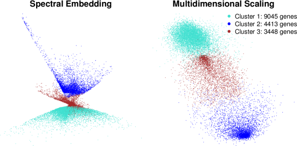
Figure 2: Two-dimensional visualization of all SENs using two different dimensionality reduction algorithms: spectral embedding [26] (left) and multidimensional scaling [27] (right). The color scheme indicates the cluster membership as determined by the PAM algorithm. Both visualizations indicate three main clusters.

All SENs were clustered into up to six clusters using the procedures outlined in Sec. II-B. The two instability analyses were each performed using $b_{\max}=500$. Using the first randomization scheme, $5\%$ of networks were randomly sampled for node permutation, while in the second procedure $20\%$ of networks were randomly sampled and white noise was introduced by adding $\pm 20\%$ to each edge weight. The results for all three clustering procedures, Tab. I, show that PAM clustering has the lowest instability followed by fuzzy C-means. Furthermore, for all three clustering methods grouping data into two and three clusters leads to the lowest instabilities.

TABLE I: Different stability analyses for three different clustering algorithms using two randomization strategies (vertex and edge permutation).

	Vertex permutation			Edge perturbation
$I_{\text{norm}}(k)$	PAM	Cmeans	k-means	PAM	Cmeans	k-means
$I_{\text{norm}}(2)$	0.016	0.020	0.065	0.009	0.015	0.065
$I_{\text{norm}}(3)$	0.018	0.023	0.076	0.010	0.016	0.071
$I_{\text{norm}}(4)$	0.023	0.031	0.092	0.019	0.033	0.180
$I_{\text{norm}}(5)$	0.026	0.038	0.171	0.025	0.030	0.191
$I_{\text{norm}}(6)$	0.031	0.080	0.187	0.027	0.086	0.208

The PAM algorithm was chosen to generate the final partitions as it yields the lowest instability index. As an additional validation to support the choice of three PAM clusters, we used three internal validation measures: the Sillhouette width [28], the Dunn index [13] and the within-cluster variance [29]. The Dunn index and Silhouette width support the presence of two to three clusters, see Tab. II. However, the intra-cluster variance, which is known to be more sensitive to the existence of sub-clusters [30], shows that grouping data into two clusters leads to high within-cluster variability compared to a higher number of clusters. By taking all these criteria into account, we have chosen to consider $k=3$ since this leads to the lowest instability and within-cluster variability whilst having as high as possible Dunn and Sillhouette scores.

TABLE II: Cluster validation measures for clustering SENs into $k$ clusters using PAM.

k	Dunn	Silhouette	Within-cluster Variance
2	2.20	0.66	0.276
3	1.20	0.44	0.225
4	0.61	0.30	0.215
5	0.63	0.23	0.223
6	0.48	0.18	0.211

In an attempt to visually assess whether this choice seems appropriate, we used a distance-preserving projection of all $16906$ SENs into a $2$D-dimensional space using two different dimensionality reduction procedures: spectral embedding [26] and multidimensional clustering [27]. The resulting projections can be found in Fig. 2. All three clusters – $1$ (turquoise), $2$ (blue) and $3$ (brown) – appear well-separated.

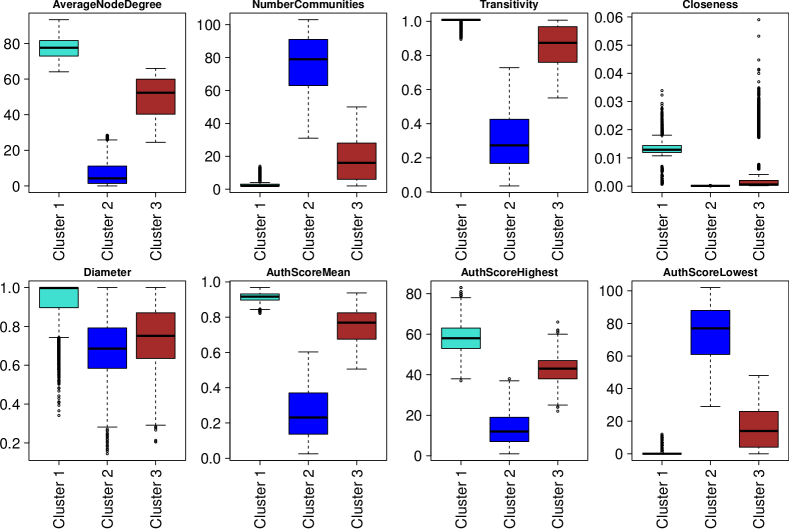
Figure 3: Distribution of topological network measures in the three clusters obtained using the PAM algorithm. High node degrees imply high edge weights with fewer low-weighted shortest paths and fewer discrepancies in edge values. This leads to high transitivity and closeness values, simultaneously reducing the number of communities SENs are partitioned into. Higher node degrees lead to more nodes having high authority scores thus increasing both the average authority scores and the number of nodes with high authority. Low node degrees signify sparseness of the SENs and more low-weighted shortest paths. This results in more nodes being grouped in their own communities, in addition to low closeness and transitivity. Sparse networks and low node degrees result in lower authority scores and fewer nodes with high authority score.

III-B Topological differences amongst SEN clusters

To validate that the three SEN clusters have distinct topological structure, we used the eight global network measures outlined in Sec. II-C. The frequency distribution of the topological measures for each cluster is summarized in Fig. 3 where a clear mean difference can be observed for each individual measure across clusters. Using a MANOVA test, we reject the null hypothesis of equality of topological features across clusters ($p<2.2e-16$; Wilk’s $\Lambda=0.3589$).

We have found that Cluster $1$ mostly consists of SENs with the highest node degree, centrality measures, diameter, authority score and number of nodes with high authority score, while there are only a few number of communities and few nodes with low authority score. These properties imply coherent expression levels across all brain regions. On the other hand, Cluster $2$ comprises of SENs with the lowest node degree, centrality measures, diameter, authority score and number of nodes with high authority scores, and the highest number of communities and nodes with low authority score. This indicates that most SENs within this cluster are sparse, and that there is high variability between expression levels across brain regions. Finally, Cluster $3$ consists of SENs with medium ranged values for all network measures, implying moderate variability between expression levels across brain regions.

III-C Biological differences amongst SEN clusters

We investigated the local transcriptomic patterns within each of the three clusters using the “coherence index” defined in Sec. II-C. The three clusters have different transcriptomic patterns, Fig. 4, and comparing heatmaps of the three clusters to one for all $16906$ genes shows that Cluster $1$ is closest to the genome-wide global patterning, while Cluster $2$ and Cluster $3$ are carriers of imposed heterogeneity. The patterns of the $16906$ genes are also consistent with existing work, and largely replicate previous findings [3, 4, 6]. In particular, homogeneity within the Neocortex and Cerebellum, and increased heterogeneity in the Basal Ganglia, have been previously reported. Cluster $2$ has few coherency patterns in the Basal Ganglia regions and Cerebellum. Cluster $1$ exhibits high homogeneity within the Cerebellum and the Neocortex, and between subdivisions of the subcortical structure and the Hippocampus. Cluster $3$ appears to have coherent patterns in the Cerebellum and the Neocortex but increased variability in the Basal Ganglia.

Obtaining detailed annotation as described in Sec. II-D revealed that all three clusters are significantly enriched ($p<0.001$) for a variety of GO BP terms. We reduced these large sets of GO terms to smaller non-redundant sets by applying REVIGO [23].

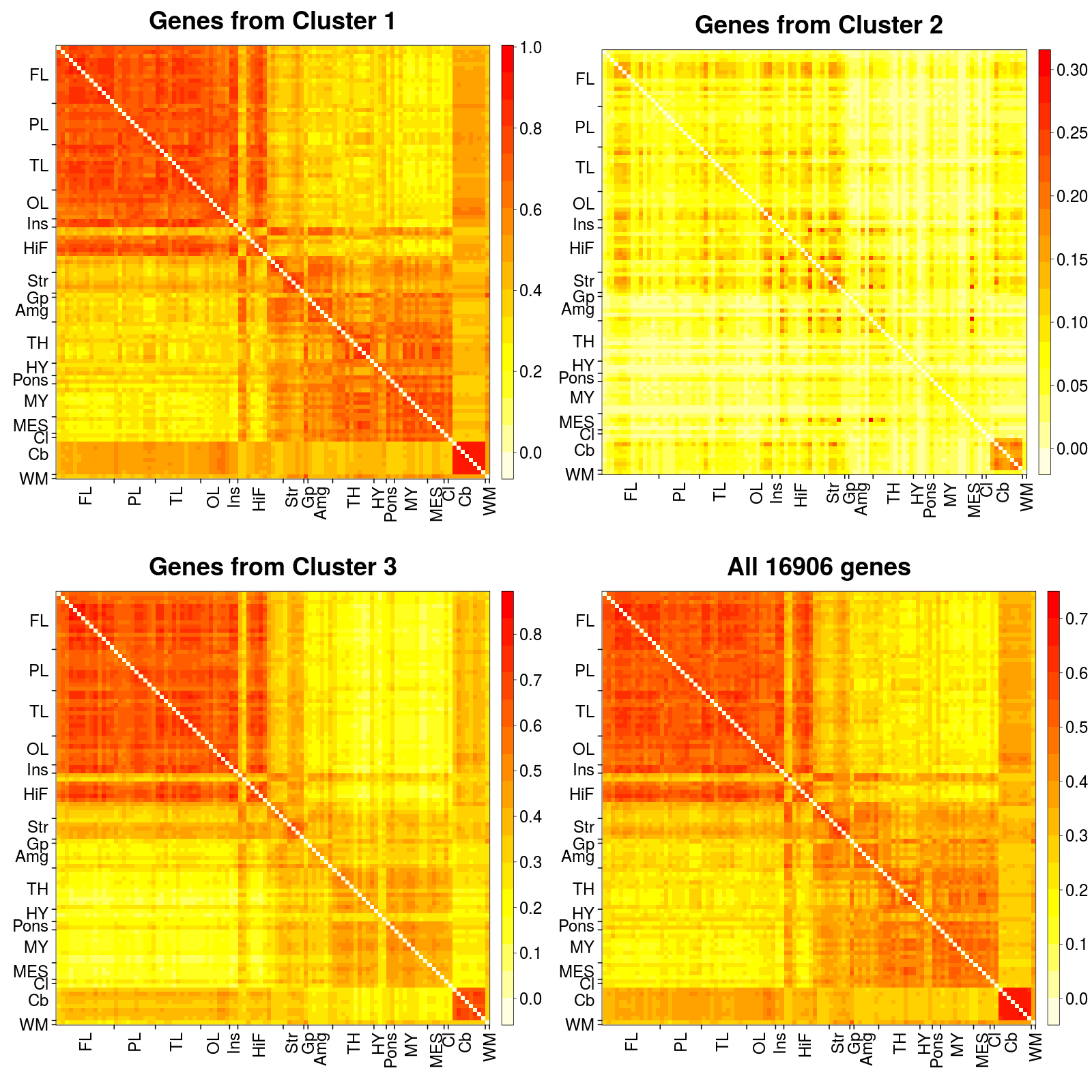
Figure 4: Heatmaps representing the “coherence index” between pairs of brain regions in each of the three SEN clusters and across all $16906$ genes. Each pixel on the heatmap is the “coherence index” between the two corresponding brain regions. Each heatmap is accompanied by a color key, where higher values indicate high homogeneity of expression levels and lower values indicate heterogeneous expression levels. The $105$ brain regions are mapped to $17$ major brain structures using the AHBA ontology atlas [8] and abbreviated as indicated in Fig. 1.

The BP representative terms selected on the basis of enrichment $p$-values and semantic similarity indicate that Cluster $1$ genes can be described primarily by “RNA processing” and “ribonucleoprotein complex biogenesis”. Cluster $2$ genes are predominantly involved in immunity including “immune system process”, “leukocyte proliferation” and “G-protein coupled receptor signaling pathway” terms primarily associated to the immune system, whereas Cluster $3$ genes are uniquely involved in “behavior”, “metal ion transport” and “nervous system development”. On closer inspection of Cluster $3$, these representative terms comprise several linked biological processes specific to the Nervous System, and which are not found on either Cluster $1$ or $2$, such as “synaptic transmission” and “dendrite extension”.

The significant disease enrichment (adjusted $p<0.001$) also supported the functional distinctiveness of the three clusters, with Cluster $1$ being enriched for Mitochondrial disease, Cluster $2$ being significantly enriched for genes involved with Immune System and Inflammatory disease, and Cluster $3$ being principally involved in Nervous system disorders. Given the observed functional differentiation between clusters, we investigated whether this might correspond to cell-type specialization. We obtained lists of neuron- and microglia-enriched genes in a repository of detailed RNA-sequencing and splicing data from purified cell cultures [31] , and computed significant intersections using the SuperExactTest [32]. This showed that genes in Cluster $3$ have significant overlap with neuron- and microglia-specific genes ($p<0.05$). Cluster $2$, on the other hand, has a unique association to microglia-specific genes only ($p<0.05$).

IV Discussion

Analyzing the transcriptome architecture of the human brain is a challenging task due to the high-dimensionality and biological complexity of the data. This is compounded by technical factors related to sample acquisition and measurement error that can influence the results. We addressed the issue of anatomical variability in gene expression by proposing to model each gene’s spatial co-expression pattern across anatomical regions as an individual spatial network, or SEN. To explore whether topological similarity of gene expression as captured by SENs is related to biological similarity, we used network dissimilarity to obtain clusters of genes with similar patterns of spatial co-expression. We aimed to gain additional insights into the biological interpretation of regional anatomical specialization of the brain.

We demonstrated that there is evidence to support the presence of three topologically distinct clusters of SENs, with each cluster being characterised by particular network properties. Furthermore, investigating the community structure of the SENs, we identified possible anatomical basis for the difference in the topological properties in the three clusters. The differences between clusters are mainly due to the heterogeneity of expression levels in the Basal Ganglia, and between the Neocortex and Cerebellum.

We also found these three topologically distinct clusters to have biologically distinct properties. On closer inspection we find Cluster $3$ to be specific to the nervous system, while Cluster $2$ appears to be involved with immunity and Cluster $1$ with transcription and translation. These associations are in line with previous results on the AHBA data set [3, 4], where the majority of clusters obtained using WGCNA [33], a well-known gene clustering procedure, were also associated to immunity, nervous system or transcription and translation.

To gain an insight into possible cellular contributions to these differences, we included cell-type specific data and observe that the overlap of neuron- and microglia- specific genes in Cluster $3$ is in keeping with current hypotheses regarding the significant interactions between these two cell-types, including the possible modulatory activity of microglia in synaptic pruning and cell communication beyond purely immune functions [34].

We found significant disease associations for all three clusters, implying the high biological impact of the genes involved and the utility of our modular clustering approach for the identification of therapeutic targets. There is a preponderance of neurological and neuropsychiatric conditions linked to Cluster $3$ genes, and immune disorders linked to Cluster $2$, reflecting their biological functions as described above and supporting those annotations.

One important concern was whether the above results were specific to using node degrees or they could be reproduced using other feature vectors. Thus we constructed two different sets of feature vectors based on node centrality as captured by the authority score and based on the raw edges of the SEN. Based on each new set of feature vectors, results not included in this paper demonstrated evidence to support the presence of three topologically distinct clusters of SENs. For both feature vectors, the three clusters were again marked by different topological properties although there were shifts in the distributions of those properties. Even so, in both cases the three clusters were uniquely associated to the immune system, nervous system or transcription and translation.

For comparison purposes, we used WGCNA on the gene expression values of the $16906$ genes for the $105$ brain regions. Results not included in this paper showed that WGCNA did not assign a cluster membership to the majority of genes in Cluster $2$ due to the sparseness of their expression levels. More and smaller clusters were discovered with higher instability. The advantage of our method compared to WGCNA is that the structure of SENs allows us to use a number of clustering procedures to detect stable gene clusters, whose validation could be achieved using both topological and biological measures. We determine the biological function of a cluster using the gene ontology of the entire set of genes in the cluster, which is robust to slight changes in the cluster membership.

A next step in the analysis of SENs should consider additional clusters to detect more specialized biological functions. Furthermore, it is well known that gene expressions in the cerebellum, subcortical and cortical regions differ significantly from each other based on their composition of different cell types [3, 4]. Future work in this direction will include an analysis where only neocortex regions are used to construct SENs.

V Conclusion

An important and challenging task in studying the brain transcriptional architecture is integrating and modelling the high dimensionality of the gene expression across the brain. To the best of our knowledge, our work is the first to perform a region-wise comprehensive profiling of gene-specific co-expression patterns across the human brain. By modelling gene expression as SENs and employing network embeddings, we identified distinct clusters of genes associated to specific biological functions, topological properties and cell-types, with potential implications for neuropsychiatric disease. Modelling genes as SENs across brain regions could be used for future studies in helping to identify genes with particular co-expression patterns across a set of spatial brain locations of interest, enabling the identification of genes that act in spatially contextualized clusters with high biological impact. As more microarray gene expression data become available at higher spatial resolution and cell-type specificity, modelling gene co-expression across the brain will be increasingly important to understanding the brain transcriptome architecture at a microstructural scale.

References

- [1] M. C. Oldham, G. Konopka, K. Iwamoto, P. Langfelder, T. Kato, S. Horvath, and D. H. Geschwind, “Functional Organization of the Transcriptome in Human Brain.,” Nat. Neurosci., vol. 11, pp. 1271–82, nov 2008.
- [2] M. Hawrylycz, L. Ng, D. Page, J. Morris, C. Lau, S. Faber, V. Faber, S. Sunkin, V. Menon, E. Lein, and A. Jones, “Multi-scale Correlation Structure of Gene Expression in the Brain.,” Neural Netw., vol. 24, pp. 933–42, nov 2011.
- [3] M. J. Hawrylycz, E. S. Lein, A. L. Guillozet-Bongaarts, E. H. Shen, L. Ng, J. A. Miller, L. N. van de Lagemaat, K. A. Smith, A. Ebbert, Z. L. Riley, C. Abajian, C. F. Beckmann, A. Bernard, D. Bertagnolli, A. F. Boe, P. M. Cartagena, M. M. Chakravarty, M. Chapin, J. Chong, and R. A. Dalley, “An Anatomically Comprehensive Atlas of the Adult Human Brain Transcriptome.,” Nature, vol. 489, pp. 391–9, sep 2012.
- [4] M. Hawrylycz, J. A. Miller, V. Menon, D. Feng, T. Dolbeare, A. L. Guillozet-Bongaarts, A. G. Jegga, B. J. Aronow, C.-K. Lee, A. Bernard, M. F. Glasser, D. L. Dierker, J. Menche, A. Szafer, F. Collman, P. Grange, and K. A. Berman, “Canonical Genetic Signatures of the Adult Human Brain.,” Nat. Neurosci., vol. 18, pp. 1832–1844, nov 2015.
- [5] J. Richiardi, A. Altmann, A.-C. Milazzo, C. Chang, M. M. Chakravarty, T. Banaschewski, G. J. Barker, A. L. W. Bokde, U. Bromberg, C. Büchel, P. Conrod, M. Fauth-Bühler, H. Flor, V. Frouin, J. Gallinat, H. Garavan, P. Gowland, A. Heinz, H. Lemaître, K. F. Mann, J.-L. Martinot, F. Nees, T. Paus, Z. Pausova, M. Rietschel, T. W. Robbins, M. N. Smolka, R. Spanagel, A. Ströhle, G. Schumann, M. Hawrylycz, J.-B. Poline, M. D. Greicius, and I. Consortium, “Correlated Gene Expression Supports Synchronous Activity in Brain Networks.,” Science, vol. 348, pp. 1241–4, jun 2015.
- [6] A. Mahfouz, M. van de Giessen, and L. van der Maaten, “Visualizing the Spatial Gene Expression Organization in the Brain through Non-linear Similarity Embeddings.,” Methods, vol. 73, pp. 79–89, mar 2015.
- [7] P. Goel, A. Kuceyeski, E. LoCastro, and A. Raj, “Spatial Patterns of Genome-wide Expression Profiles Reflect Anatomic and Fiber Connectivity Architecture of Healthy Human Brain,” Hum. Brain Mapp., vol. 35, pp. 4204–4218, aug 2014.
- [8] Allen Institute for Brain Science., “Allen Human Brain Atlas,” 2014.
- [9] Allen Human Brain Atlas, “Technical White Paper: Microarray Data Normalization,” tech. rep., Allen Institute, 2013.
- [10] G. Marsaglia, W. W. Tsang, and J. Wang, “Evaluating Kolmogorov’s Distribution,” J. Stat. Softw., vol. 8, no. 18, pp. 1–4, 2003.
- [11] L. Kaufman and P. J. Rousseeuw, Finding Groups in Data: An Introduction to Cluster Analysis. John Wiley & Sons Ltd, 1990.
- [12] U. Von Luxburg, Clustering Stability: An Overview. Now Publishers Inc., 2010.
- [13] J. C. Dunn, “A Fuzzy Relative of the ISODATA Process and Its Use in Detecting Compact Well-Separated Clusters,” J. Cybern., vol. 3, no. 3, pp. 32–57, 1973.
- [14] T. Lange, V. Roth, M. L. Braun, and J. M. Buhmann, “Stability-Based Validation of Clustering Solutions,” Neural Comput., vol. 16, no. 6, pp. 1299–1323, 2004.
- [15] M. Meila, “Comparing Clusterings — An Information Based Distance,” J. Multivar. Anal., vol. 98, pp. 873–895, may 2007.
- [16] T. Opsahl, F. Agneessens, and J. Skvoretz, “Node Centrality in Weighted Networks: Generalizing Degree and Shortest Paths,” Soc. Networks, vol. 32, pp. 245–251, jul 2010.
- [17] A. Barrat, M. Barthélemy, R. Pastor-Satorras, and A. Vespignani, “The Architecture of Complex Weighted Networks.,” Proc. Natl. Acad. Sci. U. S. A., vol. 101, pp. 3747–52, mar 2004.
- [18] J. M. Kleinberg, “Authoritative Sources in a Hyperlinked Environment,” J. ACM, vol. 46, pp. 604–632, sep 1999.
- [19] S. Scheiner, “MANOVA: Multiple Response Variables and Multispecies Interactions,” Des. Anal. Ecol. Exp., pp. 94–112, 2001.
- [20] S. Fortunato, “Community Detection in Graphs,” Phys. Rep., vol. 486, no. 3-5, pp. 75–174, 2010, 0906.0612v2.
- [21] A. Clauset, M. Newman, and C. Moore, “Finding Community Structure in Very Large Networks,” Phys. Rev. E, vol. 70, p. 066111, dec 2004, 0408187.
- [22] S. Falcon and R. Gentleman, “Using GOstats to Test Gene Lists for GO Term Association.,” Bioinformatics, vol. 23, pp. 257–8, jan 2007.
- [23] F. Supek, M. Bošnjak, N. Škunca, and T. Šmuc, “REVIGO Summarizes and Visualizes Long Lists of Gene Ontology Terms.,” PLoS One, vol. 6, p. e21800, jan 2011.
- [24] B. Zhang, S. Kirov, and J. Snoddy, “WebGestalt: An Integrated System for Exploring Gene Sets in Various Biological Contexts.,” Nucleic Acids Res., vol. 33, pp. W741–8, jul 2005.
- [25] J. Jourquin, D. Duncan, Z. Shi, and B. Zhang, “GLAD4U: Deriving and Prioritizing Gene Lists from PubMed Literature.,” BMC Genomics, vol. 13 Suppl 8, p. S20, jan 2012.
- [26] U. V. Luxburg, “A Tutorial on Spectral Clustering,” tech. rep., Max Planck Institute for Biological Cybernetics, 2007.
- [27] I. Borg and P. J. F. Groenen, Modern Multidimensional Scaling: Theory and Applications. Springer Science & Business Media, 2005.
- [28] P. J. Rousseeuw, “Silhouettes: A Graphical Aid to the Interpretation and Validation of Cluster Analysis,” J. Comput. Appl. Math., vol. 20, pp. 53–65, nov 1987.
- [29] M. Halkidi and M. Vazirgiannis, “Clustering Validity Asessment: Finding the Optimal Partitioning of a Data Set,” in Proc. 2001 IEEE Int. Conf. Data Min., pp. 187–194, IEEE Comput. Soc, 2001.
- [30] Y. Liu, Z. Li, H. Xiong, X. Gao, and J. Wu, “Understanding of Internal Clustering Validation Measures,” in 2010 IEEE Int. Conf. Data Min., pp. 911–916, IEEE, dec 2010.
- [31] Y. Zhang, K. Chen, S. A. Sloan, M. L. Bennett, A. R. Scholze, S. O’Keeffe, H. P. Phatnani, P. Guarnieri, C. Caneda, N. Ruderisch, S. Deng, S. A. Liddelow, C. Zhang, R. Daneman, T. Maniatis, B. A. Barres, and J. Q. Wu, “An RNA-Sequencing Transcriptome and Splicing Database of Glia, Neurons, and Vascular Cells of the Cerebral Cortex.,” J. Neurosci., vol. 34, pp. 11929–47, sep 2014.
- [32] M. Wang, Y. Zhao, and B. Zhang, “Efficient Test and Visualization of Multi-Set Intersections.,” Sci. Rep., vol. 5, p. 16923, jan 2015.
- [33] S. Horvath, Weighted Network Analysis: Applications in Genomics and Systems Biology. Springer, 2011.
- [34] M.-È. Tremblay, R. L. Lowery, and A. K. Majewska, “Microglial Interactions with Synapses are Modulated by Visual Experience.,” PLoS Biol., vol. 8, p. e1000527, jan 2010.