Saliency-Guided Complexity Control
for HEVC Decoding

Abstract

The latest High Efficiency Video Coding (HEVC) standard significantly improves coding efficiency over its previous video coding standards. The expense of such improvement is enormous computational complexity, from both encoding and decoding sides. Since computational capability and power capacity are diverse across portable devices, it is necessary to reduce decoding complexity to a target with tolerable quality loss, so called complexity control. This paper proposes a Saliency-Guided Complexity Control (SGCC) approach for HEVC decoding, which reduces the decoding complexity to the target with minimal perceptual quality loss. First, we establish the SGCC formulation to minimize perceptual quality loss at the constraint on reduced decoding complexity, which is achieved via disabling Deblocking Filter (DF) and simplifying Motion Compensation (MC) of some non-salient Coding Tree Units (CTUs). One important component in this formulation is the modelled relationship between decoding complexity reduction and DF disabling/MC simplification, which determines the control accuracy of our approach. Another component is the modelled relationship between quality loss and DF disabling/MC simplification, responsible for optimizing perceptual quality. By solving the SGCC formulation for a given target complexity, we can obtain the DF and MC settings of each CTU, and then decoding complexity can be reduced to the target. Finally, the experimental results validate the effectiveness of our SGCC approach, from the aspects of control performance, complexity-distortion performance, fluctuation of quality loss and subjective quality.

I Introduction

I-A Background

High Efficiency Video Coding (HEVC) standard [1] was officially approved in April 2013, significantly improving the efficiency of video coding. It is able to save around $60\%$ bit rates with similar subjective quality [2], compared with its former H.264/AVC standard. However, the cost of bit rate saving in HEVC is the huge computational complexity [3], from the aspects of both encoding and decoding. It is thus necessary to reduce encoding and decoding complexity of HEVC. The past couple of years have witnessed extensive works [4, 5, 6, 7, 8, 9, 10] on encoding complexity reduction for HEVC. Unfortunately, there are relatively few approaches on reducing HEVC decoding complexity. Actually, decoding is far more common than encoding for existing coding standards including HEVC. For example, according to [11], the amount of videos encoded and uploaded to YouTube is only around 65 thousands every day, while there are about 100 millions videos are decoded and viewed everyday. The number of decoded videos is more than 1,000 times of encoded videos. Therefore, the study on complexity reduction is more urgent for decoding.

Moreover, different devices may be diverse in computational capability. For example, the computational capability of laptops (e.g, MacBook) is probably over twice higher than that of tablets (e.g., iPad) [12]. Therefore, HEVC decoding need to be adaptive to diverse computational capability. That is, it is necessary to study on reducing HEVC decoding complexity to a target, via developing complexity control approach. Unfortunately, to our best knowledge, there exists few works on complexity control for HEVC decoding. In this paper, we propose an efficient approach to achieve this goal.

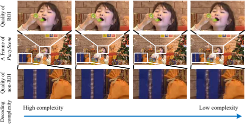
Figure 1: An example of our SGCC approach. Note that each column corresponds to a specific target for HEVC decoding complexity reduction.

I-B Related works

In early time, there existed a handful of studies [13, 14] on decoding complexity reduction, for the previous H.264/AVC standard. Most recently, several approaches [15, 16, 17, 18, 19, 20, 21, 22, 23, 24] have been proposed to reduce decoding complexity/time, for the latest HEVC standard. Among them, there are two main research directions: hardware-based and algorithmic approaches.

Some works, such as [15, 16, 17, 18, 19, 20], have been devoted to accelerating the HEVC decoding speed using hardware techniques. For example, Yan et al. [15] and Chi et al. [16] proposed to take advantage of Single Instruction Multiple Data (SIMD) instructions for increasing HEVC decoding speed. Souza et al. [17] achieved the HEVC decoding acceleration, which benefits from the parallel computing of Graphics Processing Unit (GPU). Similarly, [25] presented a new parallelization approach for accelerating HEVC decoding speed with higher frame rate. The above approaches can save HEVC decoding time in some specific hardware, but they cannot reduce the complexity and power consumed by HEVC decoding. For reducing power consumption, [13] and [26] were proposed to dynamically adjust the frequency of CPU, taking advantage of Dynamic Voltage and Frequency Scaling (DVFS) technology. As such, the decoding power consumption can be reduced for H.264/AVC [13] and HEVC [26], by means of the dynamic adjustment of CPU frequency. In the Field-Programmable Gate Array (FPGA) platform, [20] achieved the power reduction in HEVC decoding, by designing a high-performance intra prediction hardware based on Verilog Hardware Description Language (Verilog HDL). However, all these approaches can be merely implemented on the specific hardware (e.g., GPU with SIMD, DVFS, FPGA, etc.) at the decoder side, and they are hardly adaptive to generic hardware.

For overcoming the drawback of hardware-based approaches, some algorithmic approaches have been developed to decrease video decoding complexity, via simplifying some encoding/decoding components. These approaches include [14, 21, 22, 23, 24]. For H.264/AVC, Liu et al. [14] proposed to detect Region-of-Interest (ROI), and to allocate less computational resources to non-ROIs. Specifically, the total decoding complexity can be reduced with simplified coding components, according to an ROI based Rate-Distortion-Complexity (R-D-C) cost function. Later, Naccari et al. [21] proposed an approach for reducing decoding complexity of both H.264/AVC and HEVC. In [21], the offsets in Deblocking Filter (DF) are estimated with optimization on Generalized Block-edge Impairment Metric (GBIM), instead of the conventional brute force optimization. This way, the computational complexity of decoding can be saved. For HEVC, the decoding complexity is reduced in [22], by modifying the structure of prediction during encoding. However, [22] is not practical for already encoded videos, since it requires the modification at the encoder side. Most recently, [23] and [24] have been proposed to modify the components at the decoder side, to make decoding complexity reduction more practical in HEVC. To be more specific, they proposed to remove some in-loop filters, and to shorten the FIR filter sizes in Motion Compensation (MC), such that HEVC decoding complexity can be reduced. In comparison with hardware-based approaches, the algorithmic approaches on decoding complexity reduction can be implemented in any power-limited devices, but at the expense of visual quality loss.

Unfortunately, all above approaches, from both hardware-based and algorithmic aspects, cannot reduce the decoding complexity to a given target, leading to insufficient or wasteful use of power resources in some portable devices. There are only a few works on controlling decoding complexity for video coding. For example, Langroodi et al. [27] developed a decoding complexity control approach for H.264/AVC. In [27], the decoder sends its computational resource demand to the encoder side. Then, MC is optimized at the encoder side, such that decoding complexity can be controlled at the decoder side. However, [27] can be only applied to the previous H.264/AVC standard, and it is not suitable for off-line decoding because of the communication between encoder and decode sides. To our best knowledge, there exists no approach on controlling decoding complexity for the latest HEVC standard or for off-line scenarios. More importantly, for HEVC all existing complexity reduction approaches do not take perceptual visual quality into consideration, which can be well modelled by video saliency [28, 29, 30].

I-C Our work and contributions

In this paper, we propose a Saliency-Guided Complexity Control (SGCC) approach, which controls decoding complexity of HEVC, with minimization on perceptual quality loss modelled by video saliency. In our approach, we first use the method of [31] to predict video saliency map in HEVC compression domain. Then, perceptual quality is modelled, in which Mean Square Error (MSE) is weighted with the corresponding saliency values. Second, the SGCC formulation is proposed to minimize the loss of perceptual quality, when reducing HEVC decoding complexity to the target. Since DF and MC take up large proportions in the decoding time of HEVC, the decoding complexity is reduced in our SGCC formulation by disabling DF and simplifying MC for some non-salient CTUs. Third, the relationship between decoding complexity reduction and DF disabling/MC simplification is modelled for the SGCC formulation. Similarly, the influence of DF disabling/MC simplification on visual quality is also modelled. Finally, we develop a solution to the proposed SGCC formation, such that HEVC decoding complexity can be controlled to a target, while the perceptual quality is optimized.

Fig. 1 shows an example of our SGCC approach. As seen in Fig. 1, the video quality degrades along with the reduction of decoding complexity. However, when decoding complexity reduces, our SGCC approach preserves the visual quality of ROI (e.g., face), while the quality of non-ROI degrades. As such, the perceptual quality can be optimized by our SGCC approach, when reducing decoding complexity of HEVC.

To our best knowledge, our SGCC approach is the first work to reduce decoding complexity to a target (i.e., complexity control) for HEVC, and it is also the first one to minimize perceptual quality loss in decoding complexity reduction for HEVC. This paper is an extended version of our conference paper [32], with extensive advanced works summarized as follows. (1) We propose to simplify MC in our new SGCC optimization formulation, with the well modelled relationship among MC simplification, quality degradation and complexity reduction. As a result, the Maximal Achievable Reduction (MAR) of HEVC decoding can increase from $\sim 15\%$ to $\sim 40\%$. (2) For the new SGCC optimization, an efficient solution is mathematically derived. (3) The performance of our SGCC approach is thoroughly evaluated with more test sequences, comparing approaches and evaluation metrics, than [32]. As HEVC normally has hierarchical coding structure, temporal scalability may be applied to save some decoding complexity, which drops some upper layer frames without decoding. Our SGCC approach can be combined with temporal scalability to achieve higher reduction of decoding complexity.

TABLE I: Comparison of saliency detection performance.

	Original [31]	Simplified [31]	PQFT [33]	Rudoy [34]	OBDL  [35]	Itti [36]	Fang [37]
AUC	0.80	0.78	0.64	0.75	0.75	0.67	0.78
NSS	1.27	1.19	0.48	1.10	0.96	0.45	1.26
CC	0.42	0.39	0.16	0.37	0.30	0.14	0.38

II Formulation for Saliency-Guided Complexity Control Approach

II-A Preliminary of decoding complexity

In [3], it has been verified that DF takes up 13%-27% of HEVC decoding complexity (13%-27% for x86 and 13%-20% for ARM). Hence, HEVC decoding complexity can be reduced by disabling DF of some CTUs. We define $f_{n}\in\{0,1\}$ to indicate whether the DF of the $n$-th CTU is enabled ($f_{n}=0$) or disabled ($f_{n}=1$). Given saliency value $w_{n}$ of each CTU, we define $\Delta C_{D}(f_{n},w_{n})$ as the decoding complexity reduction of a frame caused by disabling the DF of the $n$-th CTU. Note that, in this paper, the decoding complexity of HEVC is measured by the computational time on a Windows PC with Inter(R) Core(TM) i7-4790K CPU.

Also, [3] has investigated that MC consumes 35%-61% of HEVC decoding complexity (37%-61% for x86 and 35%-53% for ARM). Thus, simplifying MC is an effective way to reduce HEVC decoding complexity. In MC, each sample of a CTU is calculated according to the corresponding samples in the reference frames. To save decoding complexity, the MC step can be skipped for some prediction samples. Instead, these samples are reconstructed by Nearest Neighbor (NN) interpolation from neighboring prediction samples, which are generated by the original MC step. In our method, for the $n$-th CTU, $g_{n}\in\{0,1,2,3\}$ defines that $g_{n}/4$ of each four samples are estimated by NN interpolation rather than applying MC. The remaining $(1-g_{n}/4)$ of prediction samples are decoded with the original MC step, as the reference for NN interpolation. As a result, $g_{n}$ implies the degree of simplifying MC. For example, $g_{n}=3$ indicates the highest degree of the simplification, as $3/4$ of total samples in the $n$-th CTU skip MC. $\Delta C_{M}(g_{n},w_{n})$ is defined as the decoding complexity reduction of a frame, due to simplifying MC of the $n$-th CTU.

II-B Preliminary of saliency weighted quality

As the cost of decoding complexity reduction, the visual quality of decoded videos degrades (as Fig. 2 shows). Fortunately, it has been investigated [29, 30] that visual attention of the HVS does not focus on the whole picture, but only a small region around fixation (called foveal vision). Hence, visual attention is taken into account in our approach to minimize the perceptual quality degradation.

In this paper, we use the compression domain saliency detection method [31] to directly obtain the saliency value of each CTU from HEVC bitstreams. Specifically, [31] proposed to detect saliency maps using HEVC domain features, including bits allocation, motion vectors, splitting depth and their spatial and temporal contrasts. Then, a Support Vector Machine (SVM) is learnt to combine these features for saliency detection. However, computing these complex features and applying the SVM consume high computational time, i.e., averagely 140 ms per frame. This leads to huge computational time overhead in the HEVC decoder. Since our SGCC approach aims at reducing the decoding complexity of HEVC, we simplify [31] to significantly reduce the time overhead of saliency detection.

We simplify [31] according to the two facts verified by both [31] and our experiments. (1) Bits allocation and its spatial contrast make the most essential contribution to the accuracy of saliency detection; (2) Replacing the SVM with a linear combination slightly reduces the accuracy of saliency detection, but saving extensive computational time. Therefore, the saliency value of the $n$-th CTU, defined as $w_{n}$, is detected by the linear combination of bits allocation and its spatial contrast, such that the computational time can be significantly reduced with slight accuracy loss of saliency detection. That is, $w_{n}$ is calculated by

$$\small w_{n}=\frac{1}{2}(\frac{b_{n}}{b_{max}}+\frac{\Delta b_{n}}{\Delta b_{max}}),$$ (1)

where $b_{n}$ and $\Delta b_{n}$ indicate allocated bits and spatial contrast of bit allocation for the $n$-th CTU, respectively. In addition, $b_{max}$ and $\Delta b_{max}$ are defined as the maximal values of $b_{n}$ and $\Delta b_{n}$ in a frame. In (1), $\Delta b_{n}$ is calculated as follows,

$$\small\Delta b_{n}=\left(\frac{\sum\nolimits_{n^{{}^{\prime}}\in\textbf{I}}\exp(-\frac{d_{n^{\prime}}^{2}}{2\sigma_{b}^{2}})(b_{n^{{}^{\prime}}}-b_{n})^{2}}{\sum\nolimits_{n^{{}^{\prime}}\in\textbf{I}}\exp(-\frac{d_{n^{\prime}}^{2}}{2\sigma_{b}^{2}})}\right)^{\frac{1}{2}},$$ (2)

where I is the set of 8-neighboring CTUs, and $d_{n^{\prime}}$ is the Euclidean distance between the $n^{\prime}$-th and $n$-th CTUs in pixel domain. After our simplification, saliency detection only consumes 0.058 ms time overhead per 1080p frame, much less than HEVC decoding complexity.

Moreover, we evaluate the performance of both the original and simplified version of [31] in terms of Area Under Receiver Operating Characteristic Curve (AUC), Normalized Scanpath Saliency (NSS) and linear Correlation Coefficient (CC) [38]. The evaluation is tested over all the 15 (excluding 10-bit) sequences from Classes A-D of JCT-VC databse [39]. The averaged AUC, NSS and CC for the simplified version of [31] is 0.78, 1.19 and 0.39, respectively. They are slightly lower than the original version of [31] (AUC = 0.80, NSS = 1.27 and CC = 0.42), but over 2000 times computational time can be saved.

Furthermore, we also compare the performance of the simplified and original versions of [31] with other state-of-the-art saliency detection methods. The results are shown in Table I. It can be seen that the performance of the simplified version of [31] is comparable to or even better than other state-of-the-art saliency detection methods.

Then, we follow [40] to weight the MSE of each CTU using its saliency value. Assuming that there are in total $N$ CTUs at a video frame, the Saliency Weighted MSE (SW-MSE) of this frame is calculated by

$$\small\Delta S_{n}(f_{n},g_{n},w_{n})=\frac{w_{n}}{\sum_{n=1}^{N}w_{n}}\text{MSE}(f_{n},g_{n}).$$ (3)

In (3), $\text{MSE}(f_{n},g_{n})$ is the MSE between CTUs decoded by original HEVC and by HEVC with our appraoch (when the parameters are $f_{n}$ and $g_{n}$). Note that there exists $\Delta S_{n}(f_{n}=0,g_{n}=0,w_{n})=0$, due to the fact that CTUs decoded by original HEVC are the same as those by our approach with $f_{n}=0$ and $g_{n}=0$. In the following, we focus on minimizing the SW-MSE when reducing decoding complexity. This way, the Quality of Experience (QoE) can be ensured.

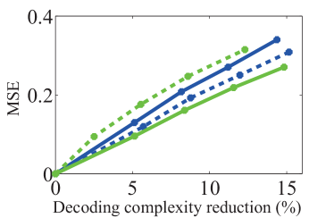
(a) Disabling DF

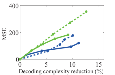
(b) Simplifying MC

Figure 2: MSE versus complexity reduction by (a) disabling DF and (b) simplifying MC for different sequences at QP = 22. Other QPs have similar results. The settings for decoding are the same as the experiments of Section V. The figures are obtained by setting (a) $f_{n}=1$ and (b) $g_{n}=3$ for some randomly selected CTUs, and setting $f_{n}=0$ and $g_{n}=0$ for other CTUs.

II-C Formulation for SGCC approach

Our SGCC approach aims at controlling the reduction of decoding complexity to the target, meanwhile minimizing perceptual quality loss (in terms of SW-MSE). Here, $\Delta S_{n}(f_{n},g_{n},w_{n})$ and $\Delta C_{n}(f_{n},g_{n},w_{n})$ are the SW-MSE and complexity reduction of the $n$-th CTU in a frame. $\Delta C_{T}$ is the target of complexity reduction. The optimization formulation of SGCC can be expressed by

$$\small\min_{{\{f_{n},g_{n}\}}_{n=1}^{N}}\!\!\sum_{n=1}^{N}\!\!\Delta S_{n}(f_{n},g_{n},w_{n})\ \ \text{s.t.}\ \sum_{n=1}^{N}\!\!\Delta C_{n}(f_{n},g_{n},w_{n})\!\!\geq\!\!\Delta C_{T},$$ (4)

where $N$ is the total number of CTUs in a frame.

Next, we discuss how to decompose $\Delta C_{n}(f_{n},g_{n},w_{n})$ and $\Delta S_{n}(f_{n},g_{n},w_{n})$ in our SGCC approach, which is the first step to solve the SGCC formulation of (4). For the decomposition, we have the following Observations.

$\mathbf{Observation}$ 1

$\Delta C_{D}(f_{n},w_{n})$ and $\small\Delta C_{M}(g_{n},w_{n})$ are almost independent with each other. Mathematically, it holds for

$$\small\sum_{n=1}^{N}\!\Delta C_{n}(f_{n},g_{n},w_{n})\!\approx\!\sum_{n=1}^{N}\!\Big{(}\!\Delta C_{D}(f_{n},w_{n})\!+\!\Delta C_{M}(g_{n},w_{n})\!\Big{)}.\!\!\!\!$$ (5)

Analysis 1

For (5), the error rate of complexity reduction can be measured:

$$\scriptsize\Delta C_{e}\!\!=\!\!\left|\!\frac{\sum_{n=1}^{N}\!\!\Delta C_{n}(f_{n},g_{n},w_{n})\!\!-\!\!\sum_{n=1}^{N}\!\!\Big{(}\!\Delta C_{D}(f_{n},w_{n})\!\!+\!\!\Delta C_{M}(g_{n},w_{n})\!\Big{)}}{\sum_{n=1}^{N}\!\!\Delta C_{n}(f_{n},g_{n},w_{n})}\!\right|.\!\!\!\!\!\!$$ (6)

If $\Delta C_{e}\rightarrow 0$, then (5) can be obtained. Here, Table II reports $\Delta C_{e}$ of decoding several videos at QP = 22, 27, 32 and 37. Note that the settings for decoding are the same as the experiments of Section V. As can be seen from Table II, almost all average $\Delta C_{e}$ is less than 1.5%. Thus, we can find $\Delta C_{e}\rightarrow 0$, and this verifies Observation 1. $\blacksquare$

$\mathbf{Observation}$ 2

Assume that $\Delta S_{D}(f_{n},w_{n})$ and $\Delta S_{M}(g_{n},w_{n})$ are the SW-MSEs of disabling DF and simplifying MC, respectively. They are almost independent with each other. Mathematically, it holds for

$$\small\sum_{n=1}^{N}\!\Delta S_{n}(f_{n},g_{n},w_{n})\!\approx\!\sum_{n=1}^{N}\!\Big{(}\!\Delta S_{D}(f_{n},w_{n})\!+\!\Delta S_{M}(g_{n},w_{n})\!\Big{)}.\!\!\!\!$$ (7)

Analysis 2

For (7), the error rate of SW-MSE can be measured:

$$\scriptsize\Delta S_{e}\!\!=\!\left|\!\frac{\sum_{n=1}^{N}\!\!\Delta\!S_{n}(f_{n},g_{n},w_{n})\!\!-\!\!\sum_{n=1}^{N}\!\Big{(}\!\Delta S_{D}(f_{n},w_{n})\!\!+\!\!\Delta S_{M}(g_{n},w_{n})\!\Big{)}}{\sum_{n=1}^{N}\!\Delta\!S_{n}(f_{n},g_{n},w_{n})}\!\right|.\!\!\!\!\!\!$$ (8)

If $\Delta S_{e}\rightarrow 0$, (7) can be acquired. Table III tabulates $\Delta S_{e}$ of decoding several videos at different QPs. Note that the settings are the same as the experiments of Section V. We can see from Table III that most of average $\Delta S_{e}$ is less than 2.5%. Thus, we can conclude that $\Delta S_{e}\rightarrow 0$, and this verifies Observation 2. $\blacksquare$

Upon above two Observations, formulation (4) can be turned to

$$\min_{{\{f_{n},g_{n}\}}_{n=1}^{N}}\sum_{n=1}^{N}\Big{(}\Delta S_{D}(f_{n},w_{n})+\Delta S_{M}(g_{n},w_{n})\Big{)}$$ (9)

$$\text{s.t.}\quad\sum_{n=1}^{N}\Big{(}\Delta C_{D}(f_{n},w_{n})+\Delta C_{M}(g_{n},w_{n})\Big{)}\geq\Delta C_{T}.$$

Next, we move to learn the functions of $\Delta C_{D}(f_{n},w_{n})$, $\Delta C_{M}(g_{n},w_{n})$, $\Delta S_{D}(f_{n},w_{n})$ and $\Delta S_{M}(g_{n},w_{n})$, for solving our SGCC formulation.

TABLE II: Values of error rate $\Delta C_{e}$(%)for all training sequences

	$f_{n}=1,g_{n}=1$				$f_{n}=1,g_{n}=2$				$f_{n}=1,g_{n}=3$
QP	22	27	32	37	22	27	32	37	22	27	32	37
1	0.7	2.3	2.9	1.2	2.6	2.7	0.0	1.9	2.0	1.7	0.4	0.6
2	0.3	0.7	0.4	0.3	3.3	1.2	0.3	1.1	1.3	0.0	1.0	1.6
3	0.3	0.1	0.2	0.9	1.9	1.20	3.2	0.4	0.2	2.0	0.31	1.5
4	2.1	0.9	1.0	0.2	4.8	0.5	0.1	0.6	2.3	1.6	2.0	0.8
Ave.	0.9	1.0	1.1	0.7	3.1	1.4	0.5	1.0	1.4	1.3	0.9	1.1
1: Cactus 2: BasketballDrive 3: BQMall 4: BasketballDrill

III Relationship Modelling for SGCC approach

III-A Relationship modelling for $\Delta S_{D}(f_{n},w_{n})$, $\Delta S_{M}(g_{n},w_{n})$

According to (3) and Observation 2, $\Delta S_{D}(f_{n},w_{n})$ and $\Delta S_{M}(g_{n},w_{n})$ can be represented by

$$\Delta S_{D}(f_{n},w_{n}) =\frac{w_{n}}{\sum_{n=1}^{N}w_{n}}\text{MSE}_{D}(f_{n}),$$ (10)

$$\Delta S_{M}(g_{n},w_{n}) =\frac{w_{n}}{\sum_{n=1}^{N}w_{n}}\text{MSE}_{M}(g_{n}).$$

In (10), $\text{MSE}_{D}(f_{n})$ is defined as the MSE between CTUs, decoded by our approach with $f_{n}\in\{0,1\}$ and by original HEVC (i.e., $f_{n}=0$). Similarly, $\text{MSE}_{M}(g_{n})$ is the MSE between the CTUs decoded by our approach with $g_{n}\in\{0,1,2,3\}$ and by original HEVC (i.e., $g_{n}=0$).

It is intractable to model $\text{MSE}_{D}(f_{n})$ and $\text{MSE}_{M}(g_{n})$ of (10), since they vary hugely across video content. However, we can use $w_{n}\frac{\text{MSE}_{D}(f_{n})}{\text{MSE}_{D}(f_{n}=1)}$ and $w_{n}\frac{\text{MSE}_{M}(g_{n})}{\text{MSE}_{M}(g_{n}=3)}$ instead of $w_{n}\text{MSE}_{D}(f_{n})$ and $w_{n}\text{MSE}_{M}(g_{n})$, respectively, since their correlation is rather high. Specifically, we evaluate the Spearman Rank Correlation Coefficient (SRCC) between $w_{n}\text{MSE}_{D}(f_{n})$ and $w_{n}\frac{\text{MSE}_{D}(f_{n})}{\text{MSE}_{D}(f_{n}=1)}$ among all CTUs for each frame. The SRCC averaged over all frames of four training sequences is 0.92. Similarly, the averaged SRCC between $w_{n}\text{MSE}_{M}(g_{n})$ and $w_{n}\frac{\text{MSE}_{M}(g_{n})}{\text{MSE}_{M}(g_{n}=3)}$ is 0.70. Consequently, on the basis of (10), the normalization can be written by

$$\small\Delta\widetilde{S}_{D}(f_{n},w_{n})\!=\!\frac{\Delta S_{D}(f_{n},w_{n})}{\Delta S_{D}(f_{n}\!=\!1,w_{n}\!=\!1)}\!=\!w_{n}\frac{\text{MSE}_{D}(f_{n})}{\text{MSE}_{D}(f_{n}\!=\!1)}$$ (11)

and

$$\small\Delta\widetilde{S}_{M}(g_{n},w_{n})\!=\!\frac{\Delta S_{M}(g_{n},w_{n})}{\Delta S_{M}(g_{n}\!=\!3,w_{n}\!=\!1)}\!=\!w_{n}\frac{\text{MSE}_{M}(g_{n})}{\text{MSE}_{M}(g_{n}\!=\!3)},$$ (12)

since $w_{n}=1$, $f_{n}=1$ and $g_{n}=3$ make SW-MSE largest in HEVC decoding. Recall that $w_{n}$ of each CTU can be obtained using the saliency detection method of [31]. Thus, we focus on estimating $\frac{\text{MSE}_{D}(f_{n})}{\text{MSE}_{D}(f_{n}=1)}$ and $\frac{\text{MSE}_{M}(g_{n})}{\text{MSE}_{M}(g_{n}=3)}$ for $\Delta\widetilde{S}_{D}(f_{n},w_{n})$ and $\Delta\widetilde{S}_{M}(g_{n},w_{n})$.

TABLE III: Values of error rate $\Delta S_{e}$(%) for all training sequences

	$f_{n}=1,g_{n}=1$				$f_{n}=1,g_{n}=2$				$f_{n}=1,g_{n}=3$
QP	22	27	32	37	22	27	32	37	22	27	32	37
1	1.6	2.6	3.5	5.1	1.0	1.3	1.6	2.6	0.0	0.4	0.7	1.0
2	2.1	2.8	3.8	3.1	0.7	1.2	1.6	2.1	0.1	0.4	0.8	1.2
3	0.6	1.7	2.5	4.3	0.3	0.8	1.1	1.9	0.1	0.4	0.7	1.3
4	0.8	1.6	2.2	3.1	0.4	1.2	1.6	2.3	0.1	0.5	0.7	1.0
Ave.	1.3	2.1	3.0	3.9	0.6	1.1	1.5	2.2	0.1	0.4	0.7	1.1
1: Cactus 2: BasketballDrive 3: BQMall 4: BasketballDrill

First, we deal with the estimation on $\frac{\text{MSE}_{D}(f_{n})}{\text{MSE}_{D}(f_{n}=1)}$. Obviously, if $f_{n}=1$, we have $\frac{\text{MSE}_{D}(f_{n})}{\text{MSE}_{D}(f_{n}=1)}=1$. If $f_{n}=0$, DF is enabled such that we have $\frac{\text{MSE}_{D}(f_{n})}{\text{MSE}_{D}(f_{n}=1)}=0$. Therefore, the following function holds,

$$\small\frac{\text{MSE}_{D}(f_{n})}{\text{MSE}_{D}(f_{n}=1)}=\left\{\begin{aligned} 0&,&\quad\text{if}\ f_{n}=0,\\ 1&,&\quad\text{if}\ f_{n}=1.\\ \end{aligned}\right.$$ (13)

Based on (11) and (13), we can obtain

$$\small\Delta\widetilde{S}_{D}(f_{n},w_{n})=w_{n}\cdot f_{n}.$$ (14)

Second, we discuss on learning $\frac{\text{MSE}_{M}(g_{n})}{\text{MSE}_{M}(g_{n}=3)}$ from some training sequences. Four sequences, selected from JCT-VC database [39], are used for training, including two $1920\times 1080$ sequences Cactus and BasketballDrive from Class B, as well as two $832\times 480$ sequences BQMall and BasketballDrill from Class C. The sequences are compressed by HM 16.0 at four different QPs, i.e., QP = 22, 27, 32 and 37. All settings are the same as those in Section V.

Four training sequences (at QP = 22, 27, 32 and 37) are decoded with MC skipped for $0$, $1$, $2$ and $3$ samples among each four samples, corresponding to $g_{n}=0,1,2,3$. As such, $0$, $1/4$, $1/2$ and $3/4$ of total samples are skipped for MC in each training CTU. Accordingly, for a training sequence, the MSE caused by skipping MC can be estimated by

$$\small\text{MSE}_{M}^{*}(g_{n})=\frac{1}{L}\sum_{l=1}^{L}\frac{\|\text{I}_{l}(g_{l}=g_{n})-\text{I}_{l}(g_{l}=0)\|_{2}^{2}}{P_{l}},$$ (15)

where $\textbf{I}_{l}$ denotes the sample set of the $l$-th training CTU, and $L$ is the total CTU number in the training sequence. $P_{l}$ is the number of samples in the $l$-th training CTU, and $g_{l}$ denotes the proportion of its samples with MC skipped. Given (15), $\{\text{MSE}_{M}^{*}(g_{n})\}_{g_{n}=0}^{3}$ can be obtained for each training sequence at one QP. Afterwards, $\text{MSE}_{M}^{*}(g_{n})$ is normalized by $\frac{\text{MSE}_{M}^{*}(g_{n})}{\text{MSE}_{M}^{*}(g_{n}=3)}$. Based on the samples of $\frac{\text{MSE}_{M}^{*}(g_{n})}{\text{MSE}_{M}^{*}(g_{n}=3)}$ for all training sequences at four QPs, we utilize the least-square fitting of the third-order polynomial regression to learn $\frac{\text{MSE}_{M}(g_{n})}{\text{MSE}_{M}(g_{n}=3)}$.

The fitting curve is shown in Fig. 3, each dot of which indicates a pair of $(g_{n},\frac{\text{MSE}_{M}^{*}(g_{n})}{\text{MSE}_{M}^{*}(g_{n}=3)})$ for a training sequence at one QP. Obviously, $\frac{\text{MSE}_{M}^{*}(g_{n})}{\text{MSE}_{M}^{*}(g_{n}=3)}=1$ for $g_{n}=3$ and $\frac{\text{MSE}_{M}^{*}(g_{n})}{\text{MSE}_{M}^{*}(g_{n}=3)}=0$ for $g_{n}=0$, due to $\text{MSE}_{M}^{*}(g_{n}=0)=0$. The R-square value of the fitting in Fig. 3 is 0.9980, verifying the effectiveness of the fitting model. Finally, the learnt polynomial function is as follows,

$$\small\frac{\text{MSE}_{M}(g_{n})}{\text{MSE}_{M}(g_{n}=3)}=h_{1}\cdot g_{n}^{3}+h_{2}\cdot g_{n}^{2}+h_{3}\cdot g_{n},$$ (16)

where the values of $h_{1}$, $h_{2}$ and $h_{3}$ are presented in Table IV. Consequently, (12) can be turned to

$$\small\Delta\widetilde{S}_{M}(g_{n},w_{n})=w_{n}\cdot(h_{1}\cdot g_{n}^{3}+h_{2}\cdot g_{n}^{2}+h_{3}\cdot g_{n}).$$ (17)

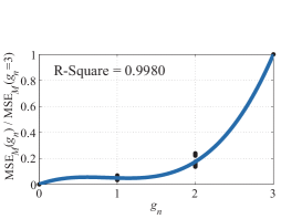
Figure 3: Fitting curve for modelling $\frac{\text{MSE}_{M}(g_{n})}{\text{MSE}_{M}(g_{n}=3)}$.

III-B Relationship Modelling for $\Delta C_{D}(f_{n},w_{n})$

Now, we move to the modelling of $\Delta C_{D}(f_{n},w_{n})$. Obviously, we have $\Delta C_{D}(f_{n}=0,w_{n})=0$, as the decoding complexity is not reduced when DF is enabled ($f_{n}=0$) for the $n$-th CTU. Next, we provide a way to learn $\Delta C_{D}(f_{n}=1,w_{n})$.

For learning $\Delta C_{D}(f_{n}=1,w_{n})$, four training sequences at four QPs are decoded with DF enabled and disabled, respectively. Then, for the $l$-th training CTU, the training sample $\Delta C^{*}_{D}(f_{l}=1,w_{l})$ can be calculated as the percentage of complexity reduction of a frame, after disabling the DF of the $l$-th training CTU. Here, $w_{l}$ is the saliency values of the $l$-th training CTU.

We apply the least-square fitting of the linear regression to estimate $\Delta C_{D}(f_{n}=1,w_{n})$ using the training data $\Delta C^{*}_{D}(f_{l}=1,w_{l})$. The fitting curves are plotted in Fig. 4. Since $\Delta C_{D}(f_{n}=1,w_{n})$ is the decoding complexity reduction of a frame caused by disabling DF of the $n$-th CTU in this frame (i.e., $f_{n}=1$), its value is also influenced by the total number of CTUs in a frame. For example, in high resolution videos, DF of one CTU occupies less decoding complexity proportion of the whole frame, than that in lower resolution videos. Such influence can be removed by multiplying $N$, and the function of $N\Delta C_{D}(f_{n}=1,w_{n})$ for different resolutions can be at the same scale and then trained together. For training $N\Delta C_{D}(f_{n}=1,w_{n})$, $N\Delta C^{*}_{D}(f_{l}=1,w_{l})$ of 3,000 randomly chosen CTUs are used as training samples, and each dot in Fig. 4 stands for one sample of $(w_{l},N\Delta C^{*}_{D}(f_{l}=1,w_{l}))$. Here, the configurations of the encoder and decoder for training are the same as those in experiments of Section V-A. Consequently, the function of $\Delta C_{D}(f_{n},w_{n})$ is

$$\small\Delta C_{D}(f_{n},w_{n})=\frac{1}{N}\cdot(a\cdot w_{n}+b)\cdot f_{n},$$ (18)

where the values of $a$ and $b$ at different QPs are presented in Table IV. Finally, $\Delta C_{D}(f_{n},w_{n})$ can be modelled.

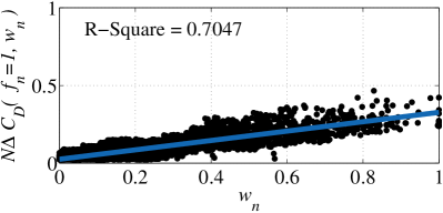
(a) QP = 22

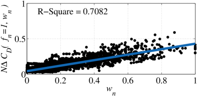
(b) QP = 27

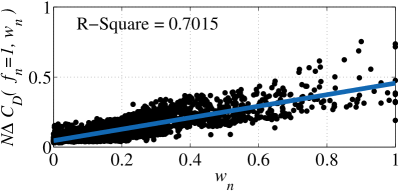
(c) QP = 32

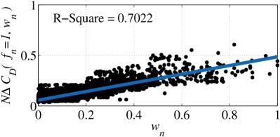
(d) QP = 37

Figure 4: Fitting curves of $w_{n}$ versus $N\Delta C_{D}(f_{n}=1,w_{n})$.

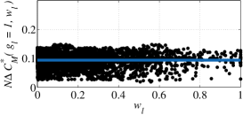
Figure 5: Pairs of $N\Delta C^{*}_{M}(g_{l}=1,w_{l})$ versus $w_{l}$ for QP = 32.

$$\small\left\{\begin{aligned} &\min_{{\{f_{n}\}}_{n=1}^{N}}\sum_{n=1}^{N}\Delta S_{D}(f_{n},w_{n})\quad\text{s.t.}\quad\sum_{n=1}^{N}\Delta C_{D}(f_{n},w_{n})\geq\Delta C_{T},\quad\quad\quad\quad\quad\quad\quad\quad\quad\quad\text{if}\ \Delta C_{T}\leq\sum_{n=1}^{N}\Delta C_{D}(f_{n}=1,w_{n}),\\ &\min_{{\{g_{n}\}}_{n=1}^{N}}\sum_{n=1}^{N}\Delta S_{M}(g_{n},w_{n})\quad\text{s.t.}\quad\sum_{n=1}^{N}\Delta C_{M}(g_{n})\geq\Delta C_{T}-\sum_{n=1}^{N}\Delta C_{D}(f_{n}=1,w_{n}),\quad\text{if}\ \Delta C_{T}>\sum_{n=1}^{N}\Delta C_{D}(f_{n}=1,w_{n}).\end{aligned}\right.$$ (21)

$$\small\left\{\begin{aligned} &\min_{{\{f_{n}\}}_{n=1}^{N}}\sum_{n=1}^{N}w_{n}\cdot f_{n}\quad\quad\quad\quad\quad\quad\quad\text{s.t.}\quad\sum_{n=1}^{N}\frac{1}{N}\cdot(a\cdot w_{n}+b)\cdot f_{n}\geq\Delta C_{T},\quad\text{if}\ \Delta C_{T}\leq\sum_{n=1}^{N}\frac{1}{N}\cdot(a\cdot w_{n}+b),\ \text{(a)}\\ &\min_{{\{g_{n}\}}_{n=1}^{N}}\sum_{n=1}^{N}w_{n}\cdot(h_{1}\cdot g_{n}^{3}+h_{2}\cdot g_{n}^{2}+h_{3}\cdot g_{n})\quad\text{s.t.}\quad\sum_{n=1}^{N}\frac{1}{N}\cdot c\cdot g_{n}\geq\Delta C^{{}^{\prime}}_{T},\quad\text{if}\ \Delta C_{T}>\sum_{n=1}^{N}\frac{1}{N}\cdot(a\cdot w_{n}+b),\ \text{(b)}\end{aligned}\right.$$ (22)

III-C Relationship Modelling for $\Delta C_{M}(g_{n},w_{n})$

Similarly, in order to model $\Delta C_{M}(g_{n},w_{n})$, four training sequences at four QPs are decoded with MC skipped for $0$, $1$, $2$ and $3$ samples among each four samples (i.e., $g_{n}=0,1,2,3$). The decoding complexity of each CTU is recorded for all training sequences. Then, we define $\Delta C^{*}_{M}(g_{l},w_{l})$ as the percentage of complexity reduction of a frame, caused by skipping MC of the $l$-th training CTU.

In Fig. 5, we plot the pairs of $N\Delta C^{*}_{M}(g_{l}=1,w_{l})$ and $w_{l}$, when decoding four training sequences at QP = 32. Note that the dots in this figure indicate the pairs of $(w_{l},N\Delta C^{*}_{M}(g_{l}=1,w_{l})$ for 3,000 randomly selected CTUs, with the same training configuration as Section III-B. Similar results can be found for other values of $g_{n}$ or other QPs. Generally speaking, this figure indicates that $\Delta C^{*}_{M}(g_{l},w_{l})$ is independent of $w_{l}$. Therefore, $\Delta C_{M}(g_{n},w_{n})$ can be replaced by $\Delta C_{M}(g_{n})$.

Next, we model $\Delta C_{M}(g_{n})$ by learning from training data of $\{\Delta C^{*}_{M}(g_{l}=g_{n})|g_{n}=0,1,2,3\}$. Sometimes, the CTU number in each training video may be dramatically different, such that the modeling of $\Delta C_{M}(g_{n},w_{n})$ may bias toward some of training video sequences. To avoid such bias, we can estimate the averaged complexity reduction of each training video sequence by

$$\small\overline{\Delta C^{*}_{M}}(g_{n})=\frac{1}{L}\sum_{l=1}^{L}\Delta C^{*}_{M}(g_{l}=g_{n}),$$ (19)

for each possible value of $g_{n}$. Recall that $L$ is the total number of CTUs on the training sequences. Then, we have $\overline{\Delta C^{*}_{M}}(g_{n})$ for each training sequence at a specific QP. For each case of a possible QP value (22, 27, 32 and 37), the least-square fitting of the linear regression is applied on all training data $N\overline{\Delta C^{*}_{M}}(g_{n})$ of four training sequences. Similar with modelling $\Delta C_{D}(f_{n},w_{n})$, we use $N\overline{\Delta C^{*}_{M}}(g_{n})$ rather than $\overline{\Delta C^{*}_{M}}(g_{n})$ here to make the regression general for different resolutions. The fitting curves are plotted in Fig. 6. Accordingly, the function of $\Delta C_{M}(g_{n})$ is obtained in the following,

$$\small\Delta C_{M}(g_{n})=\frac{1}{N}\cdot c\cdot g_{n},$$ (20)

where the values of $c$ at different QPs are presented in Table IV. Finally, $\Delta C_{M}(g_{n})$ can be modelled. It is worth pointing out that the training sequences are encoded by hierarchical GOP structure, and the frame-level QP has the offset of $0\sim+4$ (encoder_randomaccess_main.cfg). For example, when setting QP = 22, its frame-level QP ranges from 22 to 26. Therefore, in our SGCC approach, the trained parameters $a$,$b$ and $c$ for QP = 22 are to be applied for frames with QP ranging from 22 to 26. Similar setting holds for QP = 27, 32 and 37.

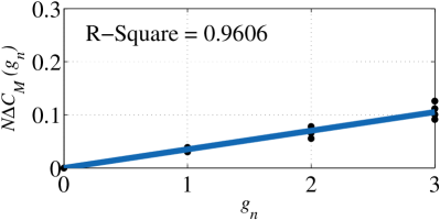
(a) QP = 22

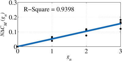
(b) QP = 27

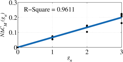
(c) QP = 32

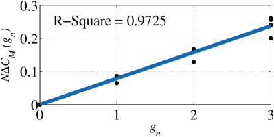
(d) QP = 37

Figure 6: Fitting curves of $g_{n}$ versus $N\Delta C_{M}(g_{n})$. Each dot indicates a pair of $(g_{n},N\overline{\Delta C^{*}_{M}}(g_{n}))$ where $g_{n}\in\{0,1,2,3\}$.

IV Solution to SGCC optimization formulation

In this section, we concentrate on solving our SGCC formulation of (9), to achieve complexity control of HEVC decoding. Since Fig. 2 has shown that the loss of MSE caused by disabling DF is significantly less than that by simplifying MC, there exists $\Delta S_{D}(f_{n},w_{n})\ll\Delta S_{M}(g_{n},w_{n})$. Therefore, in our SGCC approach, we do not simplify MC when the target complexity $\Delta C_{T}$ can be achieved by only disabling DF, i.e., $\Delta C_{T}\leq\sum_{n=1}^{N}\Delta C_{D}(f_{n}=1,w_{n})$). The MC is simplified only if $\Delta C_{T}$ cannot be satisfied by disabling DF, i.e., $\Delta C_{T}>\sum_{n=1}^{N}\Delta C_{D}(f_{n}=1,w_{n})$). As such, we can rewrite (9) of our SGCC formulation as (21). Moreover, as shown in (21), the perceptual quality loss is minimized by the optimization term, in which the DF and MC of non-salient CTUs are disabled/simplified in priority.

As discussed in Section III-A, we replace $\Delta S_{D}(f_{n},w_{n})$ and $\Delta S_{M}(g_{n},w_{n})$ of (21) by their normalized functions $\Delta\widetilde{S}_{D}(f_{n},w_{n})$ and $\Delta\widetilde{S}_{M}(g_{n},w_{n})$. Then, given the relationship of (14), (17), (18) and (20), formulation (21) can be finally turned to (22), where $\Delta C^{{}^{\prime}}_{T}=\Delta C_{T}-\sum_{n=1}^{N}\frac{1}{N}\cdot(a\cdot w_{n}+b)$.

TABLE IV: Parameters in relationship modelling for our SGCC approach.

	QP = 22	QP = 27	QP = 32	QP = 37
$h_{1}$	0.1040
$h_{2}$	-0.2737
$h_{3}$	0.2184
$a$	0.3041	0.3874	0.4101	0.4347
$b$	0.0255	0.0433	0.0459	0.0576
$c$	0.0351	0.0520	0.0665	0.0792

Given the above equations, we only need to solve (22-a) when the target complexity $\Delta C_{T}\leq\sum_{n=1}^{N}\frac{1}{N}\cdot(a\cdot w_{n}+b)$. When $\Delta C_{T}>\sum_{n=1}^{N}\frac{1}{N}\cdot(a\cdot w_{n}+b)$, we need to solve (22-b) with DF of all CTUs disabled. Once (22-a) and (22-b) are solved, the decoding complexity of HEVC can be reduced to the target by our SGCC approach, as summarized in Fig. 7. As seen from this figure, before decoding each CTU, our SGCC approach decides how to simplify MC and whether to enable DF, without any change on the CTU-level decoding pipeline. Next, we discuss how to solve (22-a) and (22-b), respectively.

IV-A Solution to formulation (22-a)

First, we aim at finding optimal solution $\textbf{F}=\{f_{n}\}_{n=1}^{N}$ of (22-a). First, let $\{\widetilde{w}_{n}\}_{n=1}^{N}$ be the set of the ascending sorted $\{w_{n}\}_{n=1}^{N}$. Given $\{\widetilde{w}_{n}\}_{n=1}^{N}$, Lemma 3 can be used for finding the optimal solution to (22-a).

$\mathbf{Lemma}$ 3

Let $a>0$, $b>0$, $l>0$ and $w_{n}\in[0,1]$. Assume that $\textbf{F}=\{f_{n}\}_{n=1}^{N}$ satisfies

$$\small f_{n}=\left\{\begin{aligned} 1&,&\quad w_{n}\leq\widetilde{w}_{I}\\ 0&,&\quad\text{otherwise},\\ \end{aligned}\right.$$ (23)

where $\tilde{w}_{I}$ is the $I$-th value of ascending sorted $\{w_{n}\}_{n=1}^{N}$. Assume that $\textbf{F}^{{}^{\prime}}=\{f^{{}^{\prime}}_{n}\}_{n=1}^{N}$ is another set with $f^{{}^{\prime}}_{n}\in\{0,1\}$.

If

$$\small\sum_{n=1}^{N}\frac{1}{N}(a\cdot w_{n}+b)\cdot f_{n}=\sum_{n=1}^{N}\frac{1}{N}(a\cdot w_{n}+b)\cdot f_{n}^{{}^{\prime}},$$ (24)

then the following inequality holds

$$\small\sum_{n=1}^{N}w_{n}\cdot f_{n}\leq\sum_{n=1}^{N}w_{n}\cdot f_{n}^{{}^{\prime}}.$$ (25)

Proof 3

The proof for Lemma 3 is in Appendix A. $\blacksquare$

According to Lemma 3, if and only if $w_{n}\leq\widetilde{w}_{I}$, $f_{n}=1$ is the optimal solution to (22-a). In order to minimize $\sum_{n=1}^{N}w_{n}\cdot f_{n}$ at the constraint of $\sum_{n=1}^{N}\frac{1}{N}(a\cdot w_{n}+b)\cdot f_{n}\geq\Delta C_{T}$, $\sum_{n=1}^{N}\frac{1}{N}(a\cdot w_{n}+b)\cdot f_{n}$ should be as close to $\Delta C_{T}$ as possible. Consequently, the optimal solution to (22-a) can be obtained as

$$\small f_{n}=\left\{\begin{aligned} 1&,&\quad w_{n}\leq\widetilde{w}_{I}\\ 0&,&\quad\text{otherwise},\\ \end{aligned}\right.$$ (26)

where $I$ satisfies

$$\small\frac{1}{N}\sum_{n=1}^{I}(a\cdot\widetilde{w}_{n}+b)\geq\Delta C_{T}>\frac{1}{N}\sum_{n=1}^{I-1}(a\cdot\widetilde{w}_{n}+b).$$ (27)

In our SGCC approach, the solution of $I$ to (27) is searched by the following way. For each frame, $a\cdot\widetilde{w}_{n}+b$ is calculated starting from $n=1$, and then added up for $n=1,2,\ldots,I$ until its sum is $\geq N\cdot\Delta C_{T}$. Once the sum $\sum_{n=1}^{I}(a\cdot\widetilde{w}_{n}+b)$ $\geq N\cdot\Delta C_{T}$, a suitable $I$ can be found out.

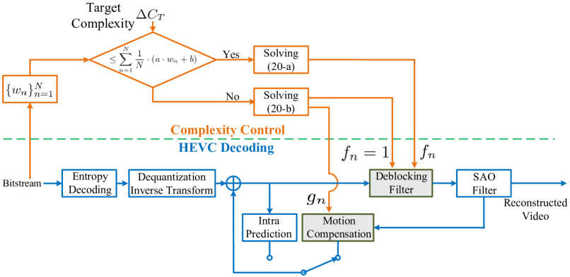
Figure 7: Framework of our SGCC approach.

IV-B Solution to formulation (22-b)

Next, we discuss on the solution to formulation (22-b). First, (22-b) can be simplified by Lemma 4.

$\mathbf{Lemma}$ 4

The nonlinear integer programming (22-b) is equivalent to the linear integer programming problem as follows,

$$\small\begin{split}&\vspace{-1em}\min_{N_{3},N_{2},N_{1}}\!\!\!\sum_{n=1}^{N_{3}}\!\!\widetilde{w}_{n}\!+\!\!\!\!\!\!\!\sum_{n=N_{3}\!+\!1}^{N_{3}\!+\!N_{2}}\!\!\!\!\!(8h_{1}\!+\!4h_{2}\!+\!2h_{3})\!\cdot\!\widetilde{w}_{n}\!\!+\!\!\!\!\!\!\!\!\!\!\!\sum_{n=N_{3}\!+\!N_{2}\!+\!1}^{N_{3}\!+\!N_{2}\!+\!N_{1}}\!\!\!\!\!\!\!\!\!(h_{1}\!+\!h_{2}\!+\!h_{3})\!\cdot\!\widetilde{w}_{n}\\ &\text{s.t.}\quad\frac{1}{N}\cdot c\cdot(N_{1}\!+\!2N_{2}\!+\!3N_{3})\geq\Delta C_{T}^{{}^{\prime}}.\end{split}$$ (28)

In (LABEL:22-b-2), $N_{1}$, $N_{2}$ and $N_{3}$ are the numbers of CTUs corresponding to $g_{n}=1,2$ and $3$ in a frame, and they satisfy $N_{1}+N_{2}+N_{3}\leq N$.

Proof 4

The proof for Lemma 4 is in Appendix B. $\blacksquare$

According to Lemma 4, the optimal solution to (22-b) can be obtained, once the formulation of (LABEL:22-b-2) is worked out. In fact, (LABEL:22-b-2) is a linear programming problem, which can be solved by the branch-and-bound algorithm [41]. However, the computational complexity of the solution is still enormous, especially for large CTU number $N$ in a frame with high resolution. It is because the branch-and-bound algorithm has to be carried out to solve (LABEL:22-b-2) for each frame. Next, we further simplify (LABEL:22-b-2) to reduce its computational complexity.

$\mathbf{Proposition}$ 5

$\widetilde{w}_{n}$ is of almost uniform distribution as follows,

$$\small\forall N_{t}\in\{n\}_{n=1}^{N},\quad\sum_{n=1}^{N_{t}}\widetilde{w}_{n}\approx k\cdot N_{t}^{2},$$ (29)

where $k$ is a positive constant.

Proof 5

The proof for Proposition 5 is in Appendix C. $\blacksquare$

Based on Proposition 5, (LABEL:22-b-2) can be rewritten by

$$\min_{N_{3},N_{2},N_{1}}N_{3}^{2}+(8h_{1}+4h_{2}+2h_{3})\cdot((N_{2}+N_{3})^{2}-N_{3}^{2})$$ (30)

$$+(h_{1}+h_{2}+h_{3})\cdot((N_{1}+N_{2}+N_{3})^{2}-(N_{2}+N_{3})^{2})$$

$$\text{s.t.}\quad\frac{1}{N}\cdot c\cdot(N_{1}+2N_{2}+3N_{3})\geq\Delta C_{T}^{{}^{\prime}}.$$

Note that $k$ is a constant which is independent of the minimization problem in (30), and thus $k$ can be simply removed from the minimization formulation.

Next, we apply the branch-and-bound algorithm [41] to solve (30), and it only needs to be solved once before decoding. We establish a table for the solutions to (30) at each specific $\Delta C_{T}^{{}^{\prime}}$. Then, given $\Delta C_{T}^{{}^{\prime}}$, we can simply obtain $N_{3},N_{2}$ and $N_{1}$ by table look-up. This way, the overhead of computational complexity on solving (22-b) can be avoided.

An example of $\{f_{n}\}_{n=1}^{N}$ and $\{g_{n}\}_{n=1}^{N}$ solved by our SGCC approach is shown in Fig. 8-(c) and (d). As can be seen , larger $f_{n}$ or $g_{n}$ corresponds to smaller $w_{n}$, which is the saliency value as illustrated in Fig. 8-(b). The detected saliency map, shown in Fig. 8-(b), tallies well with the groundtruth, i.e., the fixation map in Fig. 8-(a). As a result, the decoding complexity of CTUs in non-ROI is reduced in high priority, and the quality of ROI (e.g., face) rarely degrades. This indicates that the perceptual quality loss can be minimized in applying our SGCC approach.

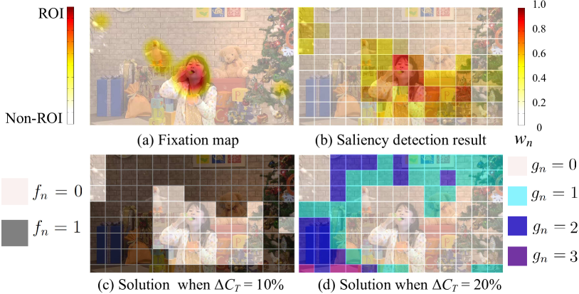
Figure 8: (a) is the fixation map (groundtruth ROI) of frame 274 in PartyScene, which is obtained from the database of [31]. (b) is the saliency detection results. (c) and (d) are example solutions of $\{f_{n}\}_{n=1}^{n}$ and $\{g_{n}\}_{n=1}^{n}$, when $\Delta C_{T}=10\%$ and $20\%$, respectively. Note that (d) only shows the values of $g_{n}$, in which the values of $f_{n}$ are all equivalent to 1.

IV-C Error propagation analysis

The quality loss of each decoded frame, which is caused by the above complexity control, may propagate to other frames predicted by this frame. Hence, it is necessary to analyze the error propagation across decoded frames. We find through the following observations that the hierarchical coding structure of HEVC can significantly alleviate the error propagation in our SGCC approach. Here, for analysis, we use the hierarchical GOP structure of the default HM Random Access (RA) with encoder_randomaccess_main.cfg file, as shown in Fig. 9. Similar results can be found for other GOP structure.

$\mathbf{Observation}$ 6

The quality loss of I frames does not incur any error propagation, when reducing decoding complexity by our SGCC approach.

Analysis 6

The reconstruction of I-frames is independent of other frames, and thus the quality loss of other frames has no impact on each decoded I frames. We further tested the error propagation of two neighboring I frames and four GOP between them (from frame 32 to frame 64), averaged over four training sequences. Here, the error propagation of the $i$-th frame is calculated as follows. First, we only apply our SGCC approach on frame $i$, and do not make any complexity reduction on other frames. Then, the quality of the $i$-th frame is evaluated by Y-PSNR in dB. For the anchor, we apply our SGCC approach on all frames, and also measure the quality of the $i$-th frame by Y-PSNR. Finally, the difference of above two PSNRs is calculated as the error propagation at frame $i$. The results are shown in Fig. 10, and we find that the PSNR reduction of each I frame is 0 dB.

Additionally, the quality loss of I frames does not incur any error propagation within the frame for our SGCC approach, as only intra prediction mode is applied in I frames. In the I-frames decoding, the DF is implemented in every frame after the reconstruction (intra prediction, etc.) of the whole frame [1]. Thus, the quality degradation caused by disabling DF cannot propagate through intra prediction among CTUs. Furthermore, since MC is only related to inter frame prediction, the error cannot propagate within I frame. This completes the validation of Observation 6.

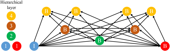
Figure 9: GOP structure and its hierarchical layers.

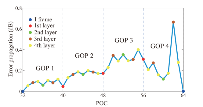
Figure 10: Averaged propagation error of each frame at QP = 32 and $\Delta C_{T}=20\%$, in terms PSNR reduction, along with Picture Order Count (POC).

$\mathbf{Observation}$ 7

The quality loss of B or P frames incurs small error propagation due to the hierarchical coding structure in HEVC, when reducing decoding complexity by our SGCC approach.

Analysis 7

In B or P frames, because of inter prediction, the quality degradation of the reference frames is possible to propagate to the currently decoded frame. Thus, error propagation exists in B or P frames. However, the error propagation is restricted to be small by the hierarchical GOP structure. First, each I frame does not incur any error propagation as pointed out by Observation 6. In addition, I frames do not have MC, such that their quality loss is only from disabling DF, which is significantly lower than that of simplifying MC (see Fig. 2). As a result, after I frames, the error propagation of B or P frames terminates, and their quality loss is resumed to be small. Second, although the B or P frames, especially in higher layers or far from I frames, suffer from error propagation, the reference frames at different layers of hierarchical coding structure ensure (see Fig. 9) that each decoded frame is predicted by several frames. Specifically, all frames of the first GOP after I frames are all predicted by I frames, which has little quality loss. Then, for the second GOP all frames have the reference frame directly predicted by I frames, such that the shortest prediction path to I frames is one frame. The shortest prediction path to I frames is two frames for the third GOP, and so on. Note that the error propagation of the frames of the GOP before an I frame can be reduced to be small, as they are also predicted by the incoming I frame. Therefore, in the hierarchical coding structure of HEVC, there exists small error propagation for the quality loss of B/P frames.

In addition, Fig. 10 shows the error propagation of all B frames between two neighboring frames averaged over four training sequences, when $\Delta C_{T}=20\%$ and QP = 32. As shown, the averaged error propagation of B frames is only 0.19 dB. Thereby, we can conclude that the error propagation of quality loss for B or P frames is rather small. Finally, the analysis of Observation 7 is completed.

Note that when applying our SGCC approach, I frames should be inserted to terminate error propagation, according to Observation 6. In this paper, the period between I frames is set as 32 for training and test sequences, according to the default configuration of encoder_randomaccess_main.cfg.

TABLE V: Individual MAR contributions ($\%$) of DF disabling and MC simplification.

Classes	Sequences	MAR of QP = 22			MAR of QP = 27			MAR of QP = 32			MAR of QP = 37
		DF	MC	SGCC	DF	MC	SGCC	DF	MC	SGCC	DF	MC	SGCC
A	Traffic	13.98	19.20	33.18	14.67	25.12	39.79	14.93	27.03	41.96	14.45	30.19	44.64
	PeopleOnStreet	15.57	9.60	25.17	19.58	11.55	31.13	21.78	12.63	34.41	20.61	17.91	38.52
B	Kimono	12.90	15.35	28.25	14.18	22.93	37.11	14.49	25.71	40.20	10.80	31.07	41.87
	ParkScene	13.47	17.12	30.59	14.33	22.47	36.80	14.89	25.21	40.10	11.55	32.39	43.94
	BQTerrace	10.98	12.66	23.64	16.18	19.84	36.02	16.14	25.88	42.02	12.83	32.40	45.23
C	RaceHorses	12.54	6.29	18.83	15.92	11.03	26.95	15.30	16.56	31.86	16.46	17.93	34.39
	PartyScene	10.67	9.71	20.38	15.81	13.28	29.09	14.28	20.73	35.01	11.27	26.74	38.01
D	RaceHorses	13.19	8.45	21.64	16.38	10.08	26.46	18.76	10.77	29.53	16.78	17.97	34.75
	BQSquare	10.72	14.60	25.32	12.36	20.49	32.85	13.70	23.55	37.25	12.48	28.34	40.82
	BlowingBubbles	10.62	12.85	23.47	12.61	16.47	29.08	14.02	18.68	32.70	15.36	21.50	36.86
	BasketballPass	12.94	10.21	23.15	15.98	12.51	28.49	17.73	13.78	31.51	15.12	20.41	35.53
Average		12.51	12.37	24.87	15.27	16.89	32.16	16.00	20.05	36.05	14.34	25.17	39.51

IV-D Complexity overhead analysis

Finally, we analyze the complexity overhead in applying our SGCC approach. The complexity overhead of our SGCC approach includes calculating $\{w_{n}\}$, computation on (22-a) and (22-b). Their computational time is evaluated and reported in Table VI. Note that the function QueryPerformanceCounter() in Visual C++ was used to record the computational time. The experiment was performed on a Windows PC with Inter(R) Core(TM) i7-4790K CPU.

It can be seen from Table VI that the complexity overhead of our SGCC approach is rather small. In particular, calculating saliency values $\{w_{n}\}$ consumes averagely 0.058 ms per 1080p frame. When calculating (22-a), saliency values $\{w_{n}\}_{n=1}^{N}$ need to be sorted as $\{\widetilde{w}_{n}\}_{n=1}^{N}$ by the quicksort algorithm, which averagely consumes 0.010 ms per 1080p frame. Besides, computing $I$ in (27) consumes averagely 0.001 ms per frame for 1080p videos for solving (22-a). For solving (22)-b, as mentioned in Section IV-B, we establish a look-up table for the solutions to (22)-b, and we can simply obtain the solution by the table look-up, when decoding HEVC bitstreams. Therefore, the computational time of (22)-b is only for reading the values $N_{1}$, $N_{2}$ and $N_{3}$ from the table, according to given $\Delta C_{T}$. Such computational time is too little to be measured. In summary, the total complexity overhead of decoding complexity control for 1080p sequences is 0.069 ms per frame, which is very little compared to DF and MC in HEVC decoding. For other resolutions, similar computational time can be found in Table VI.

Note that when applying our SGCC approach to the HEVC bitstreams with other configurations, the parameters in Table IV may need to be re-trained. However, these parameters only need to be re-trained once before applying the SGCC approach to the HEVC decoder. Consequently, re-training the parameters only introduces off-line computational time overhead, and does not consume any HEVC decoding time. In our SGCC approach, training a new set of parameters consumes around 297.40 s overhead of computational time in off-line manner.

TABLE VI: Complexity overhead of our SGCC approach per frame.

	Calculating $\{w_{n}\}_{n=1}^{N}$	Solving (22-a)	(22-b)	Total
1600p	0.119 ms	0.025 ms	-	0.144 ms
1080p	0.058 ms	0.011 ms	-	0.069 ms
480p	0.015 ms	0.002 ms	-	0.017 ms
240p	0.003 ms	0.001 ms	-	0.004 ms

V Experimental Results

In this section, experimental results are presented to validate the effectiveness of our SGCC approach, in comparison with the latest HEVC decoding complexity reduction approaches [23] and [24].

V-A Settings

All 15 sequences of Classes A-D (except 10-bit sequences) from the JCT-VC database [39] were divided into non-overlapping training and test sets. Four sequences were selected as the training set to learn the relationship of Section III. Then, we tested our approach on the remaining sequences, including two $2560\times 1600$ sequences Traffic and PeopleOnStreet from Class A, three $1920\times 1080$ sequences Kimono, ParkScene and BQTerrace from Class B, two $832\times 480$ sequences RaceHorses and PartyScene from Class C, and four $416\times 240$ sequences RaceHorses, BQSquare, BlowingBubbles and BasketballPass from Class D. First, all tested sequences were encoded by the HM 16.0 encoder. Here, the configuration of RA was implemented with GOP size being 8. Four common QPs, i.e., 22, 27, 32 and 37, were chosen to encode the test sequences. All other parameters were set by default in the encoder, using the encoder_randomaccess_main.cfg file. Besides, HM 16.0 with its default settings was also utilized as the decoder. In our experiments, our SGCC approach is implemented in the HM platform, the same as most of existing HEVC complexity reduction works [5, 6, 7, 8, 9, 10]. Compared to encoding, HM is more practical in decoding, since our experiments found that it is able to achieve real-time decoding for 1080p videos at 24 fps and QP = 37 on a Windows PC with Inter(R) Core(TM) i7-4790K CPU.

The experiments were all performed on a Windows PC with Inter(R) Core(TM) i7-4790K CPU and 32G RAM. To evaluate visual quality, both Y-PSNR difference ($\Delta\text{PSNR}$) and Eye-tracking Weighted Y-PSNR difference ($\Delta\text{EW-PSNR}$) [42] are assessed. Here, Y-PSNR and EW-PSNR are calculated upon the raw and decoded sequences. Then, $\Delta\text{PSNR}$ and $\Delta\text{EW-PSNR}$ quantify the PSNR and EW-PSNR degradation, when decoding sequences by HEVC with our SGCC, [23] and [24] approaches, instead of the original HEVC decoder. As such, the smaller $\Delta\text{PSNR}$ and $\Delta\text{EW-PSNR}$ indicate better performance in quality loss. In calculating $\Delta\text{EW-PSNR}$, we utilize human fixation maps from eye-tracking experiment to weight MSE, for fair comparison. In addition, the results of the Difference Mean Opinion Score (DMOS) [43] are also measured to assess the subjective quality of decoding sequences.

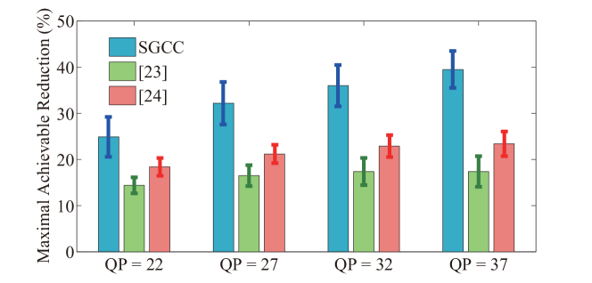
Figure 11: Mean and standard deviation of MARs for our SGCC, [23] and [24] approaches.

TABLE VII: Complexity control error of our SGCC approach.

Classes	Sequences	QP = 22		QP = 27			QP = 32			QP = 37
		$\Delta C_{T}$ (%)		$\Delta C_{T}$ (%)			$\Delta C_{T}$ (%)			$\Delta C_{T}$ (%)
		10	20	10	20	30	10	20	30	10	20	30	40
A	Traffic	+2.81	+4.46	+0.97	+3.01	+7.30	-0.19	+0.78	+4.14	+0.44	-0.29	+2.20	+4.29
	PeopleOnStreet	+3.06	-0.02	+2.10	+3.20	+1.13	+0.83	+5.06	+0.89	+2.34	+5.48	+2.12	-1.72
B	ParkScene	+1.82	+2.54	+0.57	+2.16	+7.11	+0.47	+0.87	+3.03	+1.78	+0.08	+2.05	+3.48
	BQTerrace	-1.70	-3.02	+1.57	+0.94	+6.80	+0.50	-0.45	+3.67	+1.62	-1.43	+1.89	+4.81
	Kimono	-0.72	+2.14	+1.47	+1.33	+6.02	+1.01	+1.23	+3.35	+0.60	-0.94	+0.38	+1.34
C	RaceHorses	+0.39	-3.93	+0.29	-1.14	-3.05	-0.40	+0.83	-3.83	+3.23	+2.27	-1.77	-6.09
	PartyScene	-1.78	-3.79	-1.21	-2.15	-0.91	-2.41	-1.80	-2.63	-0.57	-1.49	-1.79	-2.46
D	RaceHorses	-0.52	-3.45	-0.58	-1.26	-3.54	-0.37	1.28	-3.56	+1.74	+2.41	-1.44	-5.38
	BQSquare	-2.74	-2.15	-3.31	-1.20	+2.85	-3.14	-2.40	-0.14	-1.91	-3.22	-1.40	+0.24
	BlowingBubbles	-3.31	-3.45	-3.52	-2.57	-0.92	-3.14	-2.25	-2.98	-1.74	-2.37	-2.82	-3.20
	BasketballPass	-0.69	-2.44	-1.26	-0.53	-1.51	-1.27	+0.45	-2.77	+0.15	+0.96	-1.83	-4.56
MAE		1.78	2.85	1.53	1.77	1.94	1.25	1.58	2.82	1.46	1.90	1.79	3.42
MRE		17.78	14.26	15.32	8.86	6.45	12.47	7.91	9.39	14.60	9.50	5.97	8.55

TABLE VIII: $\Delta\text{PSNR}$ and $\Delta\text{EW-PSNR}$ (dB) at QP = 32 and 22 for SGCC, [23] and [24].

Class	Sequence	Appr.	QP=32, $\Delta\!C_{T}\!\!\!=\!\!8\%$ $/$ QP=22, $\Delta\!C_{T}\!\!\!=\!\!5\%$		QP=32, $\Delta\!C_{T}\!\!\!=\!\!18\%$ $/$ QP=22, $\Delta\!C_{T}\!\!\!=\!\!15\%$		QP=32, $\Delta\!C_{T}\!\!\!=\!\!23\%$ $/$ QP=22, $\Delta\!C_{T}\!\!\!=\!\!20\%$
			$\Delta\text{PSNR}$	$\Delta\text{EW-PSNR}$	$\Delta\text{PSNR}$	$\Delta\text{EW-PSNR}$	$\Delta\text{PSNR}$	$\Delta\text{EW-PSNR}$
A	Traffic	SGCC	0.0848 / 0.0642	0.0634 /0.0478	0.2962 / 0.5657	0.2015 / 0.2863	1.0616 / 5.7466	0.5667 / 4.5571
		[23]	0.3401 / 0.7851	0.4313 / 1.0425	1.0019 /2.2343	1.2724 /2.8351	-   /   -	-   /   -
		[24]	0.0610 / 0.1213	0.0672 / 0.1507	0.9543 / 2.2104	1.2287 / 2.8138	9.3028 / 13.7660	10.3273 / 15.0217
	PeopleOnStreet	SGCC	0.1495 / 0.1236	0.0611 / 0.0502	0.4429 / 0.6011	0.4127 / 0.3580	0.8364 / 4.9234	0.6239 / 3.5759
		[23]	0.3522 / 0.6946	0.3952 / 0.8403	0.9160 / 1.7966	1.0259 / 2.1468	-   /   -	-   /   -
		[24]	0.1135 / 0.1753	0.1232 / 0.1986	0.8036 / 1.7145	0.9098 / 2.0734	7.6765 / 12.4255	8.2545 / 13.4957
B	ParkScene	SGCC	0.0284 / 0.0451	0.0170 / 0.0612	0.4093 / 0.9248	0.3670 / 0.5026	1.0500 / 5.4168	0.7274 / 4.6220
		[23]	0.2288 / 0.6820	0.2939 / 0.7777	0.5807 / 1.6772	0.6801 / 1.7581	-   /   -	-   /   -
		[24]	0.0413 / 0.1047	0.0721 / 0.1349	0.5559 / 1.6712	0.6263 / 1.7338	6.5633 / 11.1630	6.5933 / 11.4560
	BQTerrace	SGCC	0.0152 / 0.0203	0.0069 / 0.0045	0.3236 / 1.1269	0.0601 / 0.3316	1.7257 / 6.9894	0.8471 / 6.1868
		[23]	0.4375 / 0.9351	0.4674 / 1.1097	1.2279 / 2.4650	1.2851 / 2.8457	-   /   -	-   /   -
		[24]	0.0599 / 0.1783	0.0604 / 0.1936	1.2235 / 2.4526	1.2826 / 2.8342	9.8686 / 13.1676	10.0341 / 13.9260
	Kimono	SGCC	0.1061 / 0.0846	0.0528 / 0.0604	0.3054 / 0.3357	0.3882 / 0.4299	0.4501 / 2.1454	0.5394 / 2.0825
		[23]	0.2199 / 0.3527	0.2402 / 0.3845	0.5364 / 0.8965	0.5853 / 0.9659	-   /   -	-   /   -
		[24]	0.0780 / 0.0901	0.1010 / 0.0993	0.4741 / 0.8571	0.5107 / 0.8993	4.5654 / 7.8190	4.5623 / 7.6625
C	RaceHorses	SGCC	0.0512 / 0.0909	0.0907 / 0.0816	0.3240  0.9005	0.3779 / 0.8770	0.8482 / 4.0999	0.8542 / 3.6421
		[23]	0.3050 / 0.9234	0.3316 / 0.8741	0.7213 / 2.0427	0.8007 / 1.9319	-   /   -	-   /   -
		[24]	0.0858 / 0.1999	0.0938 / 0.2091	0.6687 / 2.0220	0.7387 / 1.9026	6.3171 / 11.1323	6.7362 / 11.3829
	PartyScene	SGCC	0.0168 / 0.0148	0.0076 / 0.0063	1.0892 / 4.1913	0.2351 / 0.7267	3.4195 / 9.5478	1.0783 / 6.4582
		[23]	0.8385 / 2.7252	0.4663 / 1.7229	1.8108 / 5.2526	1.0914 / 3.6297	-   /   -	-   /   -
		[24]	0.1147 / 0.4213	0.0762 / 0.2541	1.8182 / 5.2595	1.0728 / 3.6390	9.1921 / 15.2457	7.6641 / 13.9324
D	RaceHorses	SGCC	0.0783 / 0.0542	0.0634 / 0.0574	0.2969 / 1.6244	0.2432 / 0.7723	0.8350 / 6.7330	0.7986 / 6.5464
		[23]	0.3312 / 1.1740	0.3912 / 1.4015	0.7623 / 2.5856	0.8941 / 2.9178	-   /   -	-   /   -
		[24]	0.0785 / 0.1935	0.0831 / 0.2079	0.7108 / 2.5802	0.8303 / 2.8968	6.8314 / 13.1843	7.2170 / 13.5511
	BQSquare	SGCC	0.0010 / 0.0041	0.0052 / 0.0039	1.5612 / 6.6972	0.7684 / 4.0648	5.0606 / 13.8470	3.9165 / 13.0618
		[23]	1.4420 / 3.6301	1.2487 / 3.3762	3.0622 / 6.8422	2.7089 / 6.4708	-   /   -	-   /   -
		[24]	0.1907 / 0.5886	0.1603 / 0.5216	3.0669 / 6.8397	2.7118 / 6.4708	11.9616 / 17.6653	11.5873 / 17.5664
	BlowingBubbles	SGCC	0.0181 / 0.0125	0.0101 / 0.0144	1.1739 / 5.3492	0.4200 / 2.7555	3.2883 / 11.2444	2.0604 / 10.0694
		[23]	0.5719 / 2.0708	0.4786 / 2.0190	1.2774 / 4.1821	1.1231 / 4.1169	-   /   -	-   /   -
		[24]	0.0639 / 0.2993	0.0527 / 0.2788	1.2869 / 4.1948	1.1302 / 4.1311	8.0493 / 14.1225	7.9817 / 14.4524
	BasketballPass	SGCC	0.0945 / 0.0567	0.0584 / 0.0332	0.3108 / 1.0316	0.2516 / 0.3296	0.8332 / 5.6245	0.5587 / 4.8829
		[23]	0.3041 / 1.0168	0.3048 / 1.0379	0.7798 / 2.1075	0.7836 / 2.1202	-   /   -	-   /   -
		[24]	0.0968 / 0.1751	0.0913 / 0.1934	0.7106 / 2.0762	0.7226 / 2.0924	5.5834 / 11.2566	5.3963 / 11.2870
Average		SGCC	0.0585 / 0.0519	0.0397 / 0.0383	0.5939 / 2.1226	0.3387 / 1.0395	1.7644 / 6.9380	1.1428 / 5.9714
		[23]	0.4883 / 1.3629	0.4590 / 1.3260	1.1524 / 2.9166	1.1137 / 2.8854	-   /   -	-   /   -
		[24]	0.0895 / 0.2316	0.0892 / 0.2220	1.1158 / 2.8980	1.0695 / 2.8626	7.8101 / 12.8134	7.8504 / 13.0667

V-B Evaluation on control performance

First of all, we evaluate the control performance of our SGCC approach in HEVC decoding. The performance evaluation consists of two parts: Maximal Achievable Reduction (MAR) and control error. First, we compare the MAR results of our SGCC approach with those of [23] and [24]. Here, to obtain MAR of our SGCC approach, we set $f_{n}=1$ and $g_{n}=3$ for all the CTUs to achieve the maximal decoding complexity reduction. Then, we record the ratio of such reduction as MAR. For [23] and [24], we also make their complexity reduction reach maximal values using the ways reported in [23] and [24]. Note that the complexity overhead of our approach (analyzed in Section IV-D), which is far less than HEVC decoding complexity, is included for evaluation.

MAR: Fig. 11 demonstrates the mean and standard deviation of MARs for our and conventional approaches. Here, the mean and standard deviation are calculated over all 11 test sequences at QP = 22, 27, 32 and 37. We can see from Fig. 11 that the MARs of our approach are much larger than those of [23] and [24]. Specifically, the averaged MARs of our approach are $24.9\%$, $32.2\%$, $36.0\%$ and $39.5\%$, corresponding to QP = 22, 27, 32 and 37. By contrast, the averaged MARs of [24] only reach $18.4\%$, $21.2\%$, $23.0\%$ and $23.4\%$ for QP = 22, 27, 32 and 37. Unfortunately, [23] obtains even less MARs. We can also see from Fig. 11 that larger MAR can be achieved in our SGCC approach, alongside increased QP. It is mainly due to the fact that small QP leads to much more coding bits, making entropy decoding consume higher complexity. However, even in the worst case of QP = 22, our approach has $24.9\%$ MAR in average, whereas the MARs of [23] and [24] are $14.4\%$ and $18.4\%$, respectively.

Table V reports the individual contributions of DF disabling and MC simplification in terms of MAR. It can be seen that disabling DF of all CTUs can averagely reduce HEVC decoding complexity by $12.5\%$, $15.3\%$, $16.0\%$ and $14.3\%$, corresponding to QP = 22, 27, 32 and 37, respectively. MC simplification is able to further achieve $12.4\%$, $16.9\%$, $20.0\%$ and $25.2\%$ complexity reduction. As such, the averaged MAR of our SGCC approach is able to reach $24.9\%$, $32.2\%$, $36.0\%$ and $39.5\%$, respectively, by both disabling DF and simplifying MC.

Control error: Next, we move to the evaluation of control error for our SGCC approach. Note that we do not compare with [23] and [24] in control error, since [23] and [24] are complexity reduction approaches, rather than complexity control. Table VII reports the control errors of each sequence across different complexity reduction targets (i.e., $\Delta C_{T}=10\%,20\%,30\%\ \text{and}\ 40\%$), at QP = 22, 27, 32 and 37. We can see from this table that in our approach the control error is up to $7.30\%$, while most errors are below $4.00\%$. Table VII also tabulates Mean Absolute Error (MAE) and Mean Relative Error (MRE) for each specific $\Delta C_{T}$, averaged over all 11 test sequences. It is apparent that MAEs of our approach in almost all cases are below $3.00\%$. The only exception is MAE = $3.42\%$, when $\Delta C_{T}$ is as large as $40\%$. Indeed, it is also necessary to evaluate MRE at different $\Delta C_{T}$, calculated by

$$\small\text{MRE}=\frac{\text{MAE}}{\Delta C_{T}}\times 100\%,$$ (31)

which indicates the proportion of control error with respect to $\Delta C_{T}$. We can further see from Table VII that MREs of most cases are less than $10\%$. In a conclusion, our SGCC approach performs well in control accuracy.

Note that when $\Delta C_{T}$ is less than the MAR of DF disabling (as shown in Table V), HEVC decoding complexity is reduced by only disabling DF of some CTUs. When $\Delta C_{T}$ cannot be reached by disabling DF of all the CTUs, the remaining amount of decoding complexity reduction is contributed by MC simplification.

V-C Evaluation on complexity-distortion performance

Now, we compare complexity-distortion performance of our SGCC approach with conventional approaches [23] and [24]. The quality loss caused by decoding complexity reduction is measured in terms of $\Delta\text{PSNR}$ and $\Delta\text{EW-PSNR}$. $\Delta\text{PSNR}$ reflects objective quality loss, while $\Delta\text{EW-PSNR}$ measures perceptual quality loss. Table VIII shows $\Delta\text{PSNR}$ and $\Delta\text{EW-PSNR}$ of our and other conventional approaches, when $\Delta C_{T}=8\%,18\%\ \text{and}\ 23\%$. Due to space limitation, the results of QP = 22 and 32 are provided in Table VIII.

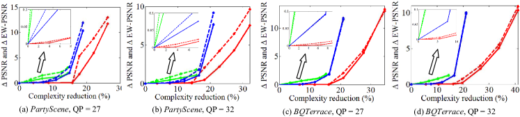
Figure 12: $\Delta\text{PSNR}$ and $\Delta\text{EW-PSNR}$ versus decoding complexity reduction at QP = 27 and 32.

Objective quality loss: It can be seen from Table VIII that Y-PSNR loss of our SGCC and other approaches increase dramatically, when decoding complexity reduction becomes larger. For example, when decoding complexity reduction increases from 8% to 18% at QP = 32, the averaged $\Delta\text{PSNR}$ of our SGCC approach enhances from 0.0585dB to 0.5939dB. Once complexity reduction reaches 23%, $\Delta\text{PSNR}$ of our approach increases to 1.7644dB. It is because MC simplification of (22-b) brings in larger distortion, in comparison with DF disabling of (22-a). It can be further seen from Table VIII that our SGCC approach significantly outperforms [23] and [24] in terms of $\Delta\text{PSNR}$, especially at high complexity reduction. Specifically, once decoding complexity reduction increases to 23%, [24] incurs averagely 7.8504dB Y-PSNR loss at QP = 32, far more than 1.7644dB of our SGCC approach. Besides, [23] is incapable of reducing decoding complexity of HEVC to 23%. Despite much better than [23] and [24], the objective quality loss of our method is not very small at high complexity reduction (e.g., $\Delta\text{PSNR}=1.7644$ dB at 23% reduction and QP = 32). However, the perceptual quality loss by our method can be alleviated (e.g., $\Delta\text{EW-PSNR}=1.1428$ dB at $23\%$ reduction and QP = 32), which is the minimization objective of our SGCC approach. For QP = 22, similar results can be found from Table VIII.

Perceptual quality loss: Table VIII shows that, for all 11 test sequences across three decoding complexity targets, $\Delta\text{EW-PSNR}$ of our SGCC approach is less than those of [23] and [24]. For example, when $\Delta C_{T}=18\%$ and QP = 32, averaged $\Delta\text{EW-PSNR}$ is 0.3387 dB, 1.1137 dB and 1.0695 dB for the SGCC, [23] and [24] approaches. This implies better perceptual quality achieved by our SGCC approach. Furthermore, the averaged values of $\Delta\text{EW-PSNR}$ are much less than those of $\Delta\text{PSNR}$ in our SGCC approach, while in [23] and [24] the values of $\Delta\text{EW-PSNR}$ are similar to those of $\Delta\text{PSNR}$. For example, the averaged $\Delta\text{PSNR}$ of our approach is 0.5939dB at $\Delta C_{T}=18\%$ and QP = 32, while $\Delta\text{EW-PSNR}$ is averagely 0.3387 dB. In contrast, the averaged values of $\Delta\text{EW-PSNR}$ and $\Delta\text{PSNR}$ are 1.1524 dB and 1.1137dB for [23], and 1.1158 dB and 1.0695 dB for [24], at $\Delta C_{T}=18\%$ and QP = 32. As shown in Table VIII, our SGCC approach also performs well in perceptual quality at QP = 22. In a word, the above results verify that our approach is capable of optimizing perceptual quality, when the decoding complexity of HEVC is reduced.

Complexity-reduction curves: To investigate the quality loss at varying reduction of decoding complexity, Fig. 12 plots the complexity-distortion curves of five selected test sequences, for our SGCC and other conventional approaches. We provide in this figure the complexity-distortion curves of QP = 27 and 32 to show the generalization of our approach at different bit rates. In Fig. 12, the curves for both $\Delta\text{PSNR}$ and $\Delta\text{EW-PSNR}$ are shown, which reflect the objective and perceptual quality loss, respectively. As shown in this figure, both $\Delta\text{PSNR}$ and $\Delta\text{EW-PSNR}$ of our SGCC approach are less than those of [23] and [24]. Besides, we can observe that $\Delta\text{EW-PSNR}$ is less than $\Delta\text{PSNR}$ in our SGCC approach, indicating better perceptual quality.

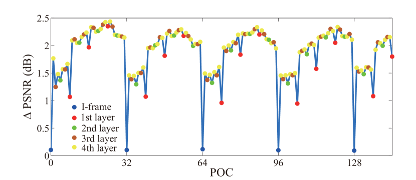
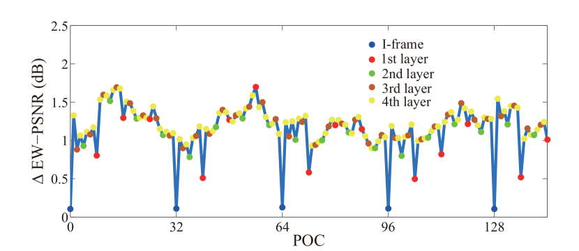
Figure 13: The frame-level $\Delta\text{PSNR}$ and $\Delta\text{EW-PSNR}$ when $\Delta C_{T}=23\%$ and QP = 32.

TABLE IX: DMOS values at QP = 32 of SGCC, [23] and [24].

$\Delta C_{T}$	Sequences	1	2	3	4	5	6	7	8	9	10	11	Average
$8\%$	SGCC	33.35	43.75	42.41	37.50	45.03	53.51	41.30	52.06	33.20	37.07	33.05	41.11
	[23]	40.79	44.28	44.25	43.47	45.79	51.40	46.20	49.97	37.90	41.76	44.70	44.59
	[24]	47.26	36.65	44.68	45.27	47.69	47.97	46.88	46.07	35.07	42.05	41.55	43.74
$23\%$	SGCC	45.98	47.23	61.06	43.33	54.81	54.43	55.07	60.83	63.06	64.37	48.22	54.40
	[24]	65.71	65.07	58.44	70.11	57.50	66.11	69.80	70.87	68.08	72.93	63.09	66.16
1: Traffic 2: PeopleOnStreet 3: ParkScene 4: BQTerrace 5: Kimono 6: RaceHorses $(832\times 480)$
7: PartyScene 8: RaceHorses $(416\times 240)$ 9: BQSquare 10: BlowingBubbles 11: BasketballPass

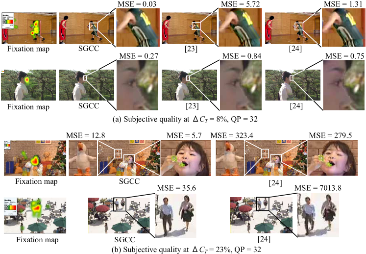
Figure 14: Subjective quality of four selected frames decoded by HEVC with our SGCC, [23] and [24] approaches, at $\Delta C_{T}=8\%$ and $\Delta C_{T}=23\%$. The MSEs of ROI in the four selected frames are given. The MSEs of our SGCC approach are significantly smaller than those of [23] and [24].

V-D Assessment on fluctuation of quality loss

Next, we assess the frame-level fluctuation of quality loss caused by our SGCC approach, since the error propagation of our approach may increase the fluctuation of quality loss. Fig. 13 plots the objective and perceptual quality loss along with decoded frames at $\Delta C_{T}=23\%$ and QP = 32, averaged over all 11 test sequences. First, it can be seen that I-frames have slight quality loss, which incur no error propagation. More importantly, the quality loss can be resumed to be near zero successively after I frames, validating the effectiveness of I frames in preventing error propagation of quality loss. This is in accordance with Observation 6. Second, the quality degradation of the frames at the first layer is less than that at upper layers, within a GOP. As such, the fluctuation of quality loss can be relieved. This indicates the small error propagation of our approach due to the hierarchical coding structure of HEVC, satisfying Observation 7. Finally, one may see that the range of $\Delta\text{EW-PSNR}$ (0.5-1.7 dB) is much smaller than that of $\Delta\text{PSNR}$ (1-2.5 dB), for non-I frames. Thus, it verifies that the perceptual quality loss of our SGCC approach has less fluctuation, compared with objective quality loss.

V-E Assessment on subjective quality

TABLE X: Complexity control error (%) of our SGCC approach for HEVC bitstreams with rate control.

Classes	Sequences	Bit rate 1		Bit rate 2		Bit rate 3			Bit rate 4
		$\Delta C_{T}$ (%)		$\Delta C_{T}$ (%)		$\Delta C_{T}$ (%)			$\Delta C_{T}$ (%)
		10	20	10	20	10	20	30	10	20	30	40
A	Traffic	+1.02	+1.08	+0.45	-0.28	+0.43	-0.82	-0.25	+0.62	-1.45	+0.79	+2.63
	PeopleOnStreet	+1.79	-0.96	+2.56	+1.67	+2.57	+3.79	-1.20	+1.77	+3.86	+0.76	-2.50
B	ParkScene	+0.90	-0.34	+1.11	-0.67	+1.50	-0.62	-0.80	+0.71	-0.83	+0.26	+1.53
	BQTerrace	-2.45	-4.39	-0.03	-1.78	+0.88	-1.75	-0.18	+0.76	-2.50	+0.40	+2.79
	Kimono	+0.82	-0.95	+0.63	-1.12	+0.08	-1.12	-1.29	-0.09	-1.74	-0.70	-0.01
C	RaceHorses	-0.63	-4.89	+1.34	-1.79	+3.03	+0.47	-5.49	+2.58	+1.26	-2.76	-6.91
	PartyScene	-2.45	-5.32	-1.44	-3.48	-0.04	-2.22	-4.96	-0.25	-2.17	-2.60	-3.40
D	RaceHorses	-0.97	-4.18	-0.08	-1.15	+0.12	+0.04	-5.24	+1.72	+1.12	-2.08	-6.73
	BQSquare	-3.16	-4.01	-2.17	-3.48	-2.42	-3.72	-3.56	-1.96	-3.70	-1.71	-1.17
	BlowingBubbles	-3.88	-5.00	-2.69	-3.62	-2.28	-3.65	-5.29	-1.87	-2.98	-2.91	-4.50
	BasketballPass	-1.71	-3.93	-1.00	-1.92	-0.58	-0.52	-4.32	-0.24	0.06	-2.16	-5.69
MAE		1.80	3.19	1.23	1.91	1.27	1.70	2.96	1.14	1.97	1.56	3.44
MRE		17.99	15.93	12.28	9.53	12.68	8.51	9.88	11.41	9.85	5.19	8.61

TABLE XI: $\Delta\text{PSNR}$ and $\Delta\text{EW-PSNR}$ (dB) of our SGCC approach for HEVC bitstreams with rate control.

Class	Sequence	Bitrate3, $\Delta\!C_{T}\!\!\!=\!\!8\%$$/$Bitrate1, $\Delta\!C_{T}\!\!\!=\!\!5\%$		Bitrate3, $\Delta\!C_{T}\!\!\!=\!\!18\%$$/$Bitrate1, $\Delta\!C_{T}\!\!\!=\!\!15\%$		Bitrate3, $\Delta\!C_{T}\!\!\!=\!\!23\%$$/$Bitrate1, $\Delta\!C_{T}\!\!\!=\!\!20\%$
		$\Delta\text{PSNR}$	$\Delta\text{EW-PSNR}$	$\Delta\text{PSNR}$	$\Delta\text{EW-PSNR}$	$\Delta\text{PSNR}$	$\Delta\text{EW-PSNR}$
A	Traffic	0.0618 / 0.0554	0.0418 / 0.0339	0.2949 / 0.6880	0.2012 / 0.3102	1.0134 / 5.4027	0.4770 / 3.8365
	PeopleOnStreet	0.1713 / 0.1141	0.0757 / 0.0460	0.5142 / 0.6207	0.4547 / 0.3026	0.8323 / 4.2424	0.6084 / 2.8400
B	ParkScene	0.0582 / 0.0380	0.0762 / 0.0490	0.3926 / 1.0378	0.3504 / 0.6955	0.9385 / 4.8877	0.7082 / 3.9699
	BQTerrace	0.0172 / 0.0175	0.0105 / 0.0086	0.4438 / 1.1507	0.1167 / 0.2280	1.8588 / 6.6625	0.8665 / 6.0677
	Kimono	0.1595 / 0.1485	0.1121 / 0.0742	0.3395 / 0.3486	0.4164 / 0.3090	0.5632 / 1.9507	0.6139 / 1.7813
C	RaceHorses	0.1077 / 0.1269	0.1081 / 0.1549	0.3323 / 0.7735	0.3195 / 0.4081	0.8656 / 5.2604	0.7179 / 4.5446
	PartyScene	0.0310 / 0.0364	0.0233 / 0.0695	1.3267 / 3.8102	0.2805 / 0.9081	3.5181 / 10.7087	1.1746 / 6.7472
D	RaceHorses	0.0909 / 0.0561	0.0706 / 0.0540	0.3112 / 1.2878	0.2393 / 0.4535	0.8652 / 5.6916	0.8331 / 5.2178
	BQSquare	0.0206 / 0.0174	0.0147 / 0.0178	1.1670 / 4.7376	0.4542 / 3.3934	3.2781 / 10.6592	2.1648 / 10.3724
	BlowingBubbles	0.0004 / 0.0036	0.0016 / 0.0036	1.4757 / 6.0610	0.8510 / 4.2087	4.7418 / 13.1899	3.7271 / 12.3745
	BasketballPass	0.1109 / 0.0539	0.0582 / 0.0391	0.4368 / 0.9602	0.3012 / 0.4422	1.0124 / 4.8030	0.6371 / 4.1436
Average		0.0754 / 0.0607	0.0539 / 0.0500	0.6395 / 1.9524	0.3623 / 1.0599	1.7716 / 6.6781	1.1390 / 5.6268

We further assess the subjective quality of our SGCC approach compared with [23] and [24]. In our experiment, the DMOS test was conducted to rate subjective quality of the decoded sequences, by the means of Single Stimulus Continuous Quality Evaluation (SSCQE), which is processed by Rec. ITU-R BT.500 [43]. During the test, sequences were displayed in random order. After viewing each decoded sequence, the subjects were asked to rate the sequence. As a result, DMOS value of each decoded sequence can be calculated to measure the difference of subjective quality between sequences decoded by original HEVC and by HEVC with our SGCC approach or other conventional approaches [23] and [24].

Table IX shows the DMOS values of three approaches for all test sequences, with complexity reduction being approximately 8% and 23%. Note that the smaller values of DMOS mean the better subjective quality, since DMOS quantifies the subjective quality difference between the uncompressed and compressed sequences. Obviously, when complexity reduction is around 8%, our SGCC approach has smaller DMOS values than [23] and [24] for 8 among 11 test sequences. Besides, the averaged DMOS value of our SGCC approach is smallest among all three approaches at $\Delta C_{T}=8\%$. Once decoding complexity is further deceased to 23%, our SGCC approach is greatly superior to [24] for all 11 test sequences, in terms of DMOS. Recall that decoding complexity reduction of [23] cannot arrive at 23%, and we thus only compare with [24] for $\Delta C_{T}=23\%$ in Table IX.

Furthermore, Fig. 14 shows some frames of four selected sequences, decoded by HEVC with the SGCC, [23] and [24] approaches. We can observe that the sequences by [23] and [24] have severe blur and blocky artifacts in ROI, at $\Delta C_{T}=8\%$. On the contrary, our SGCC approach results in better subjective quality with less blur and blocky artifacts. When $\Delta C_{T}$ is 23%, our SGCC approach enjoys more obvious quality improvement over [23] and [24], as seen in Fig. 14-(b). This is in accord with the DMOS results above.

V-F Performance on HEVC bitstreams with other configurations

In practical applications, the HEVC encoder usually enables rate control, so that frame-level QP values may vary within a sequence. Here, we further tested the trained parameters of our SGCC approach on the HEVC bitstreams encoded with rate control enabling. Here, parameters $a$, $b$ and $c$ are chosen according to the range of frame-level QP, as discussed in Section III-C. The results are shown in Tables X and XI. It can be seen that the control accuracy of decoding complexity and the degradation of quality are comparable to those without rate control (Tables VII and VIII). Note that we follow the most recent rate control work of [44] to set the target bit rates the same as the actual bit rates at fixed QPs (22, 27, 32 and 37), as reported in Tables X and XI.

We further tested the trained parameters on the HEVC bitstreams encoded with different GOP size. The results Tables XII and XIII show the results for GOP size of 4. As shown in these tables, the performance of control accuracy and quality loss of sequences are comparable to those with GOP size of 8 (Tables VII and VIII). Therefore, the parameters in Table IV are effective for the HEVC bitstreams encoded with different GOP sizes. To summarize, the trained parameters of our SGCC approach are also applicable for different encoding configurations.

TABLE XII: Complexity control error (%) of our SGCC approach for HEVC bitstreams with GOP size as 4.

Classes	Sequences	QP = 22		QP = 27			QP = 32			QP = 37
		$\Delta C_{T}$ (%)		$\Delta C_{T}$ (%)			$\Delta C_{T}$ (%)			$\Delta C_{T}$ (%)
		10	20	10	20	30	10	20	30	10	20	30	40
A	Traffic	-0.22	-0.74	-0.36	+0.04	+1.03	+1.08	-0.44	-0.93	+2.00	+0.06	+0.59	+0.21
	PeopleOnStreet	+1.76	-2.19	-0.60	+1.54	-2.28	+0.58	+1.48	+0.39	+0.62	+3.47	-0.45	-4.94
B	ParkScene	+2.61	+0.42	-0.37	-1.23	+0.19	+1.25	-0.90	+0.24	+1.35	-0.49	+0.17	-0.11
	BQTerrace	-2.15	-4.32	+1.43	+0.42	+1.57	+0.46	+0.41	-0.80	+0.80	+0.50	+1.26	+1.52
	Kimono	+1.93	-0.41	-1.42	-0.65	-1.84	-0.72	-0.51	-2.65	-1.20	-0.30	-2.96	-3.21
C	RaceHorses	-0.55	-2.53	+0.48	-2.71	-9.09	-0.40	-0.11	-3.88	+0.41	-0.87	-1.74	-8.77
	PartyScene	-1.49	-2.08	-0.64	+0.25	-4.38	+1.12	-1.21	-2.79	+1.68	+0.37	-1.04	-5.87
D	RaceHorses	-1.12	-2.10	-0.23	-2.53	-9.62	+1.61	+0.99	-3.87	-0.41	0.90	-0.94	-8.91
	BQSquare	+1.37	-0.10	-1.51	-0.89	-3.14	+0.05	+0.08	+0.49	+1.13	+0.65	+1.15	-2.35
	BlowingBubbles	+1.07	-1.81	-1.23	-2.60	-7.56	-0.06	-0.83	-3.15	+0.85	+0.60	-1.34	-7.40
	BasketballPass	-0.75	-1.18	-0.75	-2.02	-8.34	0.67	0.53	-3.30	1.43	-0.21	-1.32	-8.68
MAE		1.25	1.49	0.75	1.24	4.09	0.67	0.62	1.87	0.99	0.70	1.08	4.33
MRE		12.52	7.45	7.51	6.20	13.62	6.67	3.12	6.24	9.90	3.51	3.60	10.83

TABLE XIII: $\Delta\text{PSNR}$ and $\Delta\text{EW-PSNR}$ (dB) of our SGCC approach for HEVC bitstreams with GOP size as 4.

Class	Sequence	QP=32, $\Delta\!C_{T}\!\!\!=\!\!8\%$$/$QP=22, $\Delta\!C_{T}\!\!\!=\!\!5\%$		QP=32, $\Delta\!C_{T}\!\!\!=\!\!18\%$$/$QP=22, $\Delta\!C_{T}\!\!\!=\!\!15\%$		QP=32, $\Delta\!C_{T}\!\!\!=\!\!23\%$$/$QP=22, $\Delta\!C_{T}\!\!\!=\!\!20\%$
		$\Delta\text{PSNR}$	$\Delta\text{EW-PSNR}$	$\Delta\text{PSNR}$	$\Delta\text{EW-PSNR}$	$\Delta\text{PSNR}$	$\Delta\text{EW-PSNR}$
A	Traffic	0.1117 / 0.0955	0.0894 / 0.0594	0.4280 / 0.9878	0.3564 / 0.5921	1.3400 / 6.8979	0.8287 / 6.1152
	PeopleOnStreet	0.2307 / 0.2076	0.0969 / 0.0966	0.6619 / 1.3651	0.5962 / 0.5960	1.3069 / 8.4901	0.9758 / 7.0114
B	ParkScene	0.0934 / 0.0951	0.1250 / 0.1256	0.5035 / 1.6180	0.5662 / 0.9668	1.3820 / 7.2926	1.0978 / 6.5683
	BQTerrace	0.0342 / 0.0320	0.0182 / 0.0210	0.4270 / 1.7091	0.1038 / 0.3968	2.1345 / 8.6322	1.0791 / 8.9453
	Kimono	0.2852 / 0.1479	0.1538 / 0.0870	0.6056 / 1.1017	0.6826 / 1.1726	1.0407 / 5.7960	0.9926 / 3.9692
C	RaceHorses	0.1833 / 0.2869	0.1759 / 0.3313	0.6622 / 3.2169	0.5409 / 2.5636	1.5526 / 9.5566	1.3170 / 9.4775
	PartyScene	0.0521 / 0.0947	0.0457 / 0.2057	1.2956 / 5.3079	0.4321 / 1.6680	3.5283 / 12.3356	1.5974 / 9.9862
D	RaceHorses	0.1585 / 0.1528	0.1098 / 0.1814	0.4697 / 3.7458	0.3922 / 1.8411	1.3461 / 9.9917	1.1426 / 9.8653
	BQSquare	0.0495 / 0.0701	0.0340 / 0.0655	1.1450 / 6.5028	0.4106 / 4.8822	3.2117 / 12.1801	2.2608 / 12.2362
	BlowingBubbles	0.0099 / 0.0366	0.0128 / 0.0513	1.3174 / 8.0826	0.8062 / 6.2948	4.7982 / 14.8854	4.0667 / 14.8432
	BasketballPass	0.1717 / 0.1612	0.1171 / 0.1468	0.5093 / 1.8775	0.4551 / 0.9101	1.0825 / 8.2459	0.8343 / 8.2901
Average		0.1255 / 0.1255	0.0890 / 0.1247	0.7296 / 3.2287	0.4857 / 1.9895	2.0658 / 9.4822	1.4721 / 8.8462

VI Conclusion

This paper has proposed a decoding complexity control approach (namely SGCC) for HEVC, aiming to reduce HEVC decoding complexity to a target with minimal loss on perceptual quality. We found two ways to reduce the decoding complexity of some CTUs: (1) disabling DF and (2) simplifying MC. However, disabling DF or simplifying MC may cause some visual quality loss in decoded videos. Thus, the SGCC formulation was proposed to reduce HEVC decoding complexity to the target, meanwhile minimizing perceptual quality loss. In this paper, perceptual quality loss was evaluated on the basis of video saliency. For our formulation, the least square fitting on training data was applied to model the relationship between complexity reduction/quality loss and DF disabling/MC simplification. Finally, a potential solution to the proposed formulation was developed, such that SGCC can be accomplished for HEVC decoding. As verified in experimental results, our SGCC approach is efficient in complexity control for HEVC decoding, evaluated in control performance, complexity-distortion performance, fluctuation of quality loss, and subjective quality.

Our work in current form is implemented on HEVC RA bitstreams with hierarchical and open GOP structure. It is an interesting future work to apply our work on other settings, like close GOP structure or LD scenario. Moreover, in current stage, our SGCC approach only concentrates on LCU level complexity control for HEVC decoding. It is another promising future work to control HEVC decoding complexity at frame level, which may make our SGCC approach more flexible for controlling decoding complexity.

Appendix A Proof for Lemma 3

First, upon (23), $I=\sum_{n=1}^{N}f_{n}$ holds. Defining $M=\sum_{n=1}^{N}f^{{}^{\prime}}_{n}$, we can turn (24) to

$$a\cdot\left(\sum_{n=1}^{N}w_{n}\cdot f_{n}\right)+I\cdot b=a\cdot\left(\sum_{n=1}^{N}w_{n}\cdot f^{{}^{\prime}}_{n}\right)+M\cdot b.$$ (32)

If $I\geq M$, then $I\cdot b\geq M\cdot b$ exists due to $b>0$. Given $I\cdot b\geq M\cdot b$ and (32), we can obtain (25) because $a>0$. Therefore, for the proof of (25), we only need to prove $I\geq M$.

Next, we prove $I\geq M$ by contradiction as follows. In the case of $I<M$, we have $\sum_{n=1}^{N}f_{n}<\sum_{n=1}^{N}f^{{}^{\prime}}_{n}$. Because $f_{n}=1$ holds if and only if $w_{n}$ ($\in\left[0,1\right]$) belongs to the smallest $I$ values in $\{w_{n}\}_{n=1}^{N}$, the following inequality exists,

$$\sum_{n=1}^{N}w_{n}\cdot f_{n}<\sum_{n=1}^{N}w_{n}\cdot f^{{}^{\prime}}_{n}.$$ (33)

When $I<M$ and $b>0$, it is obvious that $I\cdot b<M\cdot b$ holds. Then, given $a>0$, we can obtain

$$a\cdot\left(\sum_{n=1}^{N}w_{n}\cdot f_{n}\right)+I\cdot b<a\cdot\left(\sum_{n=1}^{N}w_{n}\cdot f^{{}^{\prime}}_{n}\right)+M\cdot b.$$ (34)

However, (34) contradicts with (32). Hence, the assumption of $I<M$ dose not hold, such that $I\geq M$ can be proved. Finally, the inequality of (25) is achieved.

This completes the proof of Lemma 3. $\blacksquare$

Appendix B Proof for Lemma 4

First, $\sum_{n=1}^{N}g_{n}=N_{1}+2N_{2}+3N_{3}$ holds, since $N_{0}$, $N_{1}$, $N_{2}$ and $N_{3}$ are the numbers of CTUs at $g_{n}=0,1,2,3$. As such, the constraint terms of (22-b) and (28) are equivalent. Next, constraint term $\frac{1}{N}\cdot c\cdot(N_{1}+2N_{2}+3N_{3})$ of (22-b) is independent of $w_{n}$. Hence, larger $g_{n}$ should correspond to smaller $w_{n}$ to make $\sum_{n=1}^{N}w_{n}\cdot(h_{1}\cdot g_{n}^{3}+h_{2}\cdot g_{n}^{2}+h_{3}\cdot g_{n})$ minimal. This way, for each combination of $N_{0}$, $N_{1}$, $N_{2}$ and $N_{3}$, the optimal solution satisfies $\forall w_{n}\leq w_{n^{{}^{\prime}}},g_{n}\geq g_{n^{{}^{\prime}}}$. Then, the values of $N_{0}$, $N_{1}$, $N_{2}$ and $N_{3}$ are the variables to be solved for the minimization problem of (22-b). Defining $\{\widetilde{w}_{n}\}_{n=1}^{N}$ as the ascending sort of $\{w_{n}\}_{n=1}^{N}$, the optimal solution $\{g_{n}\}_{n=1}^{N}$ towards (22-b) can be written as

$$g_{n}=\left\{\begin{aligned} 3&,&\quad w_{n}\leq\widetilde{w}_{N_{3}}\\ 2&,&\quad\widetilde{w}_{N_{3}+1}\leq w_{n}\leq\widetilde{w}_{N_{3}+N_{2}}\\ 1&,&\quad\widetilde{w}_{N_{3}+N_{2}+1}\leq w_{n}\leq\widetilde{w}_{N_{3}+N_{2}+N_{1}}\\ 0&,&\quad\widetilde{w}_{N_{3}+N_{2}+N_{1}+1}\leq w_{n}\leq\widetilde{w}_{N}.\\ \end{aligned}\right.$$ (35)

Upon (22-b) and (35), we can obtain (28). Note that $h_{1}\cdot g_{n}^{3}+h_{2}\cdot g_{n}^{2}+h_{3}\cdot g_{n}=1$ when $g_{n}=3$, according to (16).

Finally, Lemma 4 can be proved. $\blacksquare$

Appendix C Proof for Proposition 5

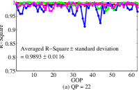
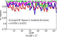
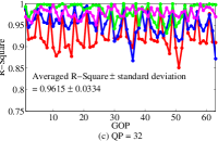
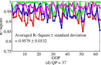
Figure 15: The R-square values for the second-order polynomial regression of $\sum_{n=1}^{N_{t}}\widetilde{w}_{n}=k\cdot N_{t}^{2}$. Note that the R-square values of the 3rd frames in each GOP are shown.

First, we apply our method of Section II to estimate the saliency values $\{w_{n}\}_{n=1}^{N}$ of all CTUs in the four training sequences (the same as Section IV) at four QPs (i.e., 22, 27, 32 and 37). Then, at each QP, the values of $\sum_{n=1}^{N_{t}}\widetilde{w}_{n}$ for all possible $N_{t}\in\{n\}_{n=1}^{N}$ are calculated and recorded at each frame of the four sequences. Recall that $\{\widetilde{w}_{n}\}_{n=1}^{N}$ is the ascending sorted set of saliency values $\{w_{n}\}_{n=1}^{N}$ for each frame. Next, we apply the second-order polynomial regression to each frame for modelling the relationship between $N_{t}$ and $\sum_{n=1}^{N_{t}}\widetilde{w}_{n}$ in form of $\sum_{n=1}^{N_{t}}\widetilde{w}_{n}=k\cdot N_{t}^{2}$, where $k$ is the second-order parameter of the regression for a video frame. Note that $k$ is a constant within a video frame, despite being different across frames. The R-square values of such regression can be obtained across different frames of four training sequences. Fig. 15 shows R-square of $\sum_{n=1}^{N_{t}}\widetilde{w}_{n}=k\cdot N_{t}^{2}$ regression along with various frames. It is evident that the R-square values are above 0.85 for all frames at four QPs. In addition, the averaged R-square values and their standard deviations are $0.9893\pm 0.0116$, $0.9709\pm 0.0252$, $0.9615\pm 0.0334$ and $0.9579\pm 0.0332$ at QP = 22, 27, 32 and 37. Thus, $\sum_{n=1}^{N_{t}}\widetilde{w}_{n}$ can be well approximated by $k\cdot N_{t}^{2}$.

Finally, Proposition 5 can be proved. $\blacksquare$

Ren Yang received the B.S. degree from Beihang University in 2012. He is currently pursuing the M.S. degree at the School of Electronic and Information Engineering, Beihang University, Beijing, China. His research interests mainly include computer vision and video coding.

Mai Xu (M’10, SM’16) received B.S. degree from Beihang University in 2003, M.S. degree from Tsinghua University in 2006 and Ph.D degree from Imperial College London in 2010. From 2010-2012, he was working as a research fellow at Electrical Engineering Department, Tsinghua University. Since Jan. 2013, he has been with Beihang University as an Associate Professor. During 2014 to 2015, he was a visiting researcher of MSRA. His research interests mainly include image processing and computer vision. He has published more than 60 technical papers in international journals and conference proceedings, e.g., IEEE TIP, CVPR and ICCV. He is the recipient of best paper awards of two IEEE conferences.

Zulin Wang (M’14) received the B.S. and M.S. degrees in electronic engineering from Beihang University, in 1986 and 1989, respectively. He received his Ph.D. degree at the same university in 2000. His research interests include image processing, electromagnetic countermeasure, and satellite communication technology. He is author or co-author of over 100 papers and holds 6 patents, as well as published 2 books in these fields. He has undertaken approximately 30 projects related to image/video coding, image processing, etc.

Yiping Duan received the B. S. degree at the school of computer science and technology, Henan Normal University, Xinxiang, China, in 2010, and Ph. D. from the school of computer science and technology, Xidian University, Xi an, China, in 2016.She is currently working towards postdoctoral research with the Department of Electronic Engineering, Tsinghua University. Her current research interests include semantic mining, machine learning and remote sensing image processing.

Xiaoming Tao (M’09) received the B.E. degree from the School of Telecommunications Engineering, Xidian University in 2003, and Ph. D. from the Department of Electronic Engineering, Tsinghua University, Beijing, China, in 2008. She is currently an Associate Professor with the Department of Electronic Engineering, Tsinghua University. Her research interests include wireless communications and networking, and multimedia signal processing.

References

- [1] G. J. Sullivan, J.-R. Ohm, W.-J. Han, and T. Wiegand, “Overview of the High Efficiency Video Coding (HEVC) standard,” IEEE TCSVT, pp. 1649–1668, 2012.
- [2] T. K. Tan, R. Weerakkody, M. Mrak, N. Ramzan, V. Baroncini, J. R. Ohm, and G. J. Sullivan, “Video quality evaluation methodology and verification testing of HEVC compression performance,” IEEE TCSVT, pp. 76–90, Jan 2016.
- [3] F. Bossen, B. Bross, K. Suhring, and D. Flynn, “HEVC complexity and implementation analysis,” IEEE TCSVT, pp. 1685–1696, 2012.
- [4] G. Correa, P. A. Assuncao, L. Volcan Agostini, and L. A. da Silva Cruz, “Fast HEVC encoding decisions using data mining,” IEEE TCSVT, pp. 660–673, 2015.
- [5] H. L. Tan, C. C. Ko, and S. Rahardja, “Fast coding quad-tree decisions using prediction residuals statistics for high efficiency video coding (HEVC),” IEEE Transactions on Broadcasting, pp. 128–133, 2016.
- [6] J. Vanne, M. Viitanen, and T. D. Hamalainen, “Efficient mode decision schemes for hevc inter prediction,” IEEE TSCVT, pp. 1579–1593, 2014.
- [7] Z. Pan, J. Lei, Y. Zhang, X. Sun, and S. Kwong, “Fast motion estimation based on content property for low-complexity h. 265/hevc encoder,” IEEE Transactions on Broadcasting, pp. 675–684, 2016.
- [8] X. Deng, M. Xu, S. Li, and Z. Wang, “Complexity control of hevc based on region-of-interest attention model,” in VCIP, 2014.
- [9] Y. Zhang, S. Kwong, X. Wang, H. Yuan, Z. Pan, and L. Xu, “Machine learning-based coding unit depth decisions for flexible complexity allocation in high efficiency video coding,” IEEE TIP, pp. 2225–2238, 2015.
- [10] X. Deng, M. Xu, L. Jiang, X. Sun, and Z. Wang, “Subjective-driven complexity control approach for HEVC,” IEEE TSCVT, 2015.
- [11] D. Dubey, A. Amritphale, A. Sawhney, D. Dubey, and N. Srivastav, “Analysis of youtube as a source of information for west nile virus infection,” Clinical medicine & research, pp. 129–132, 2014.
- [12] Everymac.com, “What are the main differences between the ipad and the macbook air?” 2014, http://www.everymac.com/.
- [13] Z. Ma, H. Hu, and Y. Wang, “On complexity modeling of h. 264/avc video decoding and its application for energy efficient decoding,” IEEE TMM, pp. 1240–1255, 2011.
- [14] Y. Liu, Z. G. Li, and Y. C. Soh, “Region-of-interest based resource allocation for conversational video communication of H.264/AVC,” IEEE TCSVT, pp. 134–139, 2008.
- [15] L. Yan, Y. Duan, J. Sun, and Z. Guo, “Implementation of HEVC decoder on x86 processors with SIMD optimization,” in VCIP, 2012.
- [16] C. C. Chi, M. Alvarez-Mesa, B. Bross, B. Juurlink, and T. Schierl, “SIMD acceleration for HEVC decoding,” IEEE TCSVT, 2014.
- [17] D. F. de Souza, A. Ilic, N. Roma, and L. Sousa, “Towards GPU HEVC intra decoding: Seizing fine-grain parallelism,” in ICME, 2015.
- [18] C. C. Chi, M. Alvarez-Mesa, B. Juurlink, G. Clare, F. Henry, S. Pateux, and T. Schierl, “Parallel scalability and efficiency of HEVC parallelization approaches,” IEEE TCSVT, pp. 1827–1838, 2012.
- [19] M. Alvarez-Mesa, C. C. Chi, B. Juurlink, V. George, and T. Schierl, “Parallel video decoding in the emerging HEVC standard,” in ICASSP, 2012.
- [20] E. Kalali, Y. Adibelli, and I. Hamzaoglu, “A high performance and low energy intra prediction hardware for hevc video decoding,” in DASIP, 2012.
- [21] M. Naccari, C. Brites, J. Ascenso, and F. Pereira, “Low complexity deblocking filter perceptual optimization for the HEVC codec,” in ICIP, 2011.
- [22] C. Feldmann, F. Jager, and M. Wien, “Decoder complexity reduction for the scalable extension of HEVC,” in ICIP, 2014.
- [23] E. Nogues, S. Holmbacka, M. Pelcat, D. Menard, and J. Lilius, “Power-aware HEVC decoding with tunable image quality,” in SIPS, 2014.
- [24] E. Nogues, E. Raffin, M. Pelcat, and D. Menard, “A modified HEVC decoder for low power decoding,” in ACM CF, 2015.
- [25] C. C. Chi, M. Alvarez-Mesa, B. Juurlink, V. George, and T. Schierl, “Improving the parallelization efficiency of hevc decoding,” in ICIP, 2012.
- [26] E. Nogues, R. Berrada, M. Pelcat, D. Menard, and E. Raffin, “A DVFS based HEVC decoder for energy-efficient software implementation on embedded processors,” in ICME, 2015.
- [27] M. J. Langroodi, J. Peters, and S. Shirmohammadi, “Decoder-complexity-aware encoding of motion compensation for multiple heterogeneous receivers,” ACM TOMM, p. 46, 2015.
- [28] C. t. Blakemore and F. Campbell, “On the existence of neurones in the human visual system selectively sensitive to the orientation and size of retinal images,” The Journal of physiology, p. 237, 1969.
- [29] W. S. Geisler and J. S. Perry, “Real-time foveated multiresolution system for low-bandwidth video communication,” in Photonics West’98 Electronic Imaging. International Society for Optics and Photonics, 1998, pp. 294–305.
- [30] Z. Wang and A. C. Bovik, “Embedded foveation image coding,” IEEE TIP, pp. 1397–1410, 2001.
- [31] M. Xu, L. Jiang, X. Sun, Z. Ye, and Z. Wang, “Learning to detect video saliency with HEVC features,” IEEE TIP, vol. 26, no. 1, pp. 369–385, 2017.
- [32] R. Yang, M. Xu, L. Jiang, and Z. Wang, “Subjective-quality-optimized complexity control for HEVC decoding,” in ICME, 2016.
- [33] C. Guo and L. Zhang, “A novel multiresolution spatiotemporal saliency detection model and its applications in image and video compression,” IEEE TIP, pp. 185–198, 2010.
- [34] D. Rudoy, D. B. Goldman, E. Shechtman, and L. Zelnik-Manor, “Learning video saliency from human gaze using candidate selection,” in CVPR, 2013.
- [35] S. H. Khatoonabadi, N. Vasconcelos, I. V. Bajic, and Y. Shan, “How many bits does it take for a stimulus to be salient?” NIPS, 2006.
- [36] L. Itti, C. Koch, and E. Niebur, “A model of saliency-based visual attention for rapid scene analysis,” IEEE TPAMI, pp. 1254–1259, 1998.
- [37] Y. Fang, W. Lin, Z. Chen, C.-M. Tsai, and C.-W. Lin, “A video saliency detection model in compressed domain,” IEEE Transactions on Circuits and Systems for Video Technology, vol. 24, no. 1, pp. 27–38, Jan. 2014.
- [38] A. Borji and I. Laurent, “State-of-the-art in visual attention modeling,” IEEE TPAMI, vol. 35, no. 1, pp. 184–207, Jan. 2013.
- [39] J.-R. Ohm, G. J. Sullivan, H. Schwarz, T. K. Tan, and T. Wiegand, “Comparison of the coding efficiency of video coding standards including high efficiency video coding (HEVC),” IEEE TCSVT, pp. 1669–1684, 2012.
- [40] Z. Wang and Q. Li, “Information content weighting for perceptual image quality assessment,” IEEE TIP, pp. 1185–1198, 2011.
- [41] D. Li and X. Sun, Nonlinear integer programming. Springer Science & Business Media, 2006.
- [42] Z. Li, S. Qin, and L. Itti, “Visual attention guided bit allocation in video compression,” Image and Vision Computing, vol. 29, no. 1, pp. 1–14, 2011.
- [43] I. Recommendation, “500-11, methodology for the subjective assessment of the quality of television pictures, Recommendation ITU-R BT. 500-11,” ITU Telecom. Standardization Sector of ITU, vol. 7, 2002.
- [44] B. Li, H. Li, L. Li, and J. Zhang, “Lambda domain rate control algorithm for high efficiency video coding,” IEEE TIP, pp. 3841–3854, 2014.