SaberLDA: Sparsity-Aware Learning of Topic Models on GPUs

Abstract

Latent Dirichlet Allocation (LDA) is a popular tool for analyzing discrete count data such as text and images. Applications require LDA to handle both large datasets and a large number of topics. Though distributed CPU systems have been used, GPU-based systems have emerged as a promising alternative because of the high computational power and memory bandwidth of GPUs. However, existing GPU-based LDA systems cannot support a large number of topics because they use algorithms on dense data structures whose time and space complexity is linear to the number of topics.

In this paper, we propose SaberLDA, a GPU-based LDA system that implements a sparsity-aware algorithm to achieve sublinear time complexity and scales well to learn a large number of topics. To address the challenges introduced by sparsity, we propose a novel data layout, a new warp-based sampling kernel, and an efficient sparse count matrix updating algorithm that improves locality, makes efficient utilization of GPU warps, and reduces memory consumption. Experiments show that SaberLDA can learn from billions-token-scale data with up to 10,000 topics, which is almost two orders of magnitude larger than that of the previous GPU-based systems. With a single GPU card, SaberLDA is able to learn 10,000 topics from a dataset of billions of tokens in a few hours, which is only achievable with clusters with tens of machines before.

1 Introduction

Topic models provide a suite of widely adopted statistical tools for feature extraction and dimensionality reduction for bag-of-words (i.e., discrete count) data, such as text documents and images in a bag-of-words format  cao2007spatially . Given an input corpus, topic models automatically extract a number of latent topics, which are unigram distributions over the words in a given vocabulary. The high-probability words in each topic are semantically correlated. Latent Dirichlet Allocation  blei2003latent (LDA) is the most popular of topic models due to its simplicity, and has been deployed as a key component in data visualization iwata2008probabilistic , text analysis boyd2007topic ; zhu2009medlda , computer vision cao2007spatially , network analysis Chang:RTM09 , and recommendation systems  chen2009collaborative .

In practice, it is not uncommon to encounter large-scale datasets, e.g., text analysis typically consists of hundreds of millions of documents  yuan2014lightlda , and recommendation systems need to tackle hundreds of millions of users  ahmed2012scalable . Furthermore, as the scale of the datasets increases, the model size needs to be increased as well — we need a larger number of topics in order to exploit the richer semantic structure underlying the data. A reasonable design goal for modern topic modeling systems is thousands of topics, to have a good coverage for both industry scale applications wang2014peacock and researching boyd2007topic ; iwata2008probabilistic ; cao2007spatially .

However, it is highly challenging to efficiently train large LDA models. The time complexity of training LDA is high because it involves iteratively scanning the input corpus for many times (e.g., 100), and the time complexity of processing each token is not constant but related to the number of topics.

Table 1: A summary of GPU-based LDA systems, $D$: the number of documents, $K$: the number of topics, $V$: the size of vocabulary, $T$: the number of tokens.

Implementation	$D$	$K$	$V$	$T$
Yan et al.  yan2009parallel	300K	128	100K	100M
BIDMach  zhao2015same	300K	256	100K	100M
Steele and Tristan  tristan2015efficient	50K	20	40K	3M
SaberLDA	19.4M	10K	100K	7.1B

To train LDA in acceptable time, CPU clusters are often used. However, due to the limited memory bandwidth and low computational power of CPUs, large clusters are typically required to learn large topic models ahmed2012scalable ; yuan2014lightlda ; yu2015scalable . For example, a 32-machine cluster is used to learn 1,000 topics from a 1.5-billion-token corpus.

A promising alternative is to train LDA with graphics processing units (GPUs), leveraging their high computational power and memory bandwidth. Along this line, there have been a number of previous attempts. For example, Yan et al. yan2009parallel implement the collapsed Gibbs sampling algorithm, BIDMach zhao2015same implements the variational Bayes algorithm as well as a modified Gibbs sampling algorithm, and Steele and Tristan tristan2015efficient propose a expectation-maximization algorithm. These GPU-based systems are reported to achieve superior performance than CPU-based systems yan2009parallel ; zhao2015same ; tristan2015efficient .

Unfortunately, current GPU-based LDA systems can only learn a few hundred topics (See Table 1), which may not be sufficient to capture the rich semantic structure underlying the large datasets in industry scale applications wang2014peacock . It is fundamentally difficult for these systems to learn more topics because they use algorithms on dense data structures whose time and space complexity is linear to the number of topics.

To address this problem, we propose SaberLDA, a novel GPU-based system that adopts a sparsity-aware algorithm for LDA. Sparsity aware algorithms are based on the insight that a single document is not likely to have many topics, and are able to achieve sub-linear (or even amortized constant) time complexity with respect to the number of topics. Representative examples include AliasLDA li2014reducing , F+LDA yu2015scalable , LightLDA yuan2014lightlda , WarpLDA chen2016warplda and ESCA zaheer2015exponential , which are implemented in general purpose CPU systems. Therefore, the running time is not sensitive with the number of topics.

However, it is considerably more challenging to design and implement sparsity-aware algorithms on GPUs than on CPUs. Comparing with CPUs, GPUs have much larger number of threads, much smaller per thread cache size and longer cache lines, which makes it much more difficult to use caches to mitigate the random access problems introduced by sparsity. The branch divergence issues of GPUs suggest we should fully vectorize the code. But for sparse data structures, loop length is no longer fixed and the data are not aligned, which indicates that straightforward vectorization is not feasible. Finally, the limited GPU memory capacity requires streaming input data and model data, which add another dimension of complexity for data partition and layout, to enable parallelism, good locality and efficient sparse matrix updates all together.

SaberLDA addresses all these challenges for supporting sparsity-aware algorithms on GPU, our key technical contribution includes:

• A novel hybrid data layout “partition-by-document and order-by-word” (PDOW) that simultaneously maximizes the locality and reduces the GPU memory consumption;

• A warp-based sampling kernel that is fully vectorized, and is equipped with a $W$-arysampling tree that supports both efficient construction and sampling;

• An efficient “shuffle and segmented count” (SSC) algorithm for updating sparse count matrices.

Our experimental results demonstrate that SaberLDA is able to train LDA models with up to 10,000 topics, which is more than an order of magnitude larger than previous GPU-based systems yan2009parallel ; zhao2015same ; tristan2015efficient , where the throughput only decreases by 17% when the number of topics increases from 1,000 to 10,000. SaberLDA is also highly efficient, under various topic settings, SaberLDA converges 5 times faster than previous GPU-based systems and 4 times faster than CPU-based systems. With a single card, SaberLDA is able to learn 10,000 topics from a dataset of billions of tokens, which is only achievable with clusters with tens of machines before yu2015scalable .

The rest the paper is organized as follows, Sec. 2 introduces the basics for LDA. Sec. 3 presents the design of SaberLDA. Sec. 4 contains the experiments and Sec. 5 concludes.

2 Latent Dirichlet Allocation

In this section, we introduce the latent Dirichlet allocation (LDA) model and its sampling algorithm.

2.1 Definition

Figure 1: An example token list and related count matrices.

LDA is a hierarchical Bayesian model that learns latent topics from text corpora blei2003latent . For an input text corpus, the scale of the learning task is determined by the following four numbers:

• $D$: the number of documents in the given corpus;

• $T$: the number of tokens, i.e., words, appearing in all the documents;

• $V$: the number of unique words in the corpus, also known as vocabulary size;

• $K$: the number of topics,

where $D$, $T$ and $V$ are determined by the corpus, and $K$ is a parameter that users can specify.

The text corpus is represented as a token list $L$, where each occurrence of word $v\in[1,V]$ in document $d\in[1,D]$ is called a token, and represented by a triplet $(d,v,k)$. While $d$ and $v$ are specified by the corpus, training LDA involves assigning a topic assignment $k\in[1,K]$ for each token $(d,v,k)$.

After the token list is given, we construct two count matrices as below:

• The document-topic count matrix $\bm{\mathbf{A}}$ is $D\times K$, where $A_{dk}$ is the number of tokens $t$ with $(d_{t}=d,k_{t}=k)$.

• The word-topic count matrix $\bm{\mathbf{B}}$ is $V\times K$, where $B_{vk}$ is the number of tokens $t$ with $(v_{t}=v,k_{t}=k)$,

where the matrix $\bm{\mathbf{A}}$ is often sparse, i.e., has many zero elements (See below for an example).

We omit the mathematical details of LDA and refer the interested readers to standard LDA literature blei2003latent ; griffiths2004finding . Informally, the LDA model is designed in a way that maximizes some objective function (the likelihood) related to the topic assignments $k$. A document $d$ can be characterized by the $d$-th row of the document-topic matrix $\bm{\mathbf{A}}$, and a topic $k$ can be characterized by the $k$-th column of the word-topic matrix $\bm{\mathbf{B}}$. Figure 1 is a concrete example, where there are $D=3$ documents, $T=8$ tokens, $V=5$ words in the vocabulary, and $K=3$ topics. Each token is assigned with a topic assignment from 1 to 3, indicated as the superscript in the figure. $\bm{\mathbf{A}}$ is the document-topic matrix, e.g., $A_{13}=2$ because both tokens in document 1 is assigned to topic 3. $\bm{\mathbf{B}}$ is the word-topic matrix, and its each column characterizes what the corresponding topic is about, e.g., the first topic has the word “apple” and “iPhone”, and is about the device iPhone; the second topic is about fruits, and the third topic is about mobile OS. Likewise, the rows of $\bm{\mathbf{A}}$ characterizes what documents are about, e.g., the first document is about mobile OS, the second document is about iPhone and mobile OS, and the last document is about fruits. Note that the matrix $\bm{\mathbf{A}}$ is sparse, because a document is not likely to be relevant with all the topics at the same time.

2.2 Inference

Given the token list $L$ , our goal is to infer the topic assignment $k_{t}$ for each token $t$. Many algorithms exist for this purpose, such as variational inference blei2003latent , Markov chain Monte-Carlo griffiths2004finding , and expectation maximization zaheer2015exponential ; chen2016warplda . We choose the ESCA algorithm zaheer2015exponential to implement on GPU for its following advantages

• It is sparsity-aware, so the time complexity is sub-linear with respect to the number of topics. This property is critical to support the efficient training of large models;

• It enjoys the best degree of parallelism because the count matrices $\bm{\mathbf{A}}$ and $\bm{\mathbf{B}}$ only need to be updated once per iteration. This matches with the massively parallel nature of GPU to achieve high performance.

The ESCA algorithm alternatively performs the E-step and the M-step for a given number of iterations (e.g., 100 iterations), where the E-step updates $k_{t}$ given the counts $\bm{\mathbf{A}},\bm{\mathbf{B}}$, and the M step updates $\bm{\mathbf{A}},\bm{\mathbf{B}}$ given $k_{t}$:

• E-step: for each token $(d,v,k)$, sample the topic assignment $k$:

  $$p(k)\propto(A_{dk}+\alpha)\hat{B}_{vk},$$ (1)

  where $\propto$ means “proportional to” and the word-topic probability matrix $\bm{\mathbf{\hat{B}}}$ is a normalized version of the count matrix $\bm{\mathbf{B}}$ in the sense that $\bm{\mathbf{\hat{B}}}$ is roughly proportional to $\bm{\mathbf{B}}$, but each of its column sums up to 1. $\hat{B}_{vk}$ is computed as follows:

  $$\hat{B}_{vk}=\frac{B_{vk}+\beta}{\sum_{v=1}^{V}B_{vk}+V\beta},$$ (2)

• M-step: update the counts $\bm{\mathbf{A}}$ and $\bm{\mathbf{B}}$, and calculate $\bm{\mathbf{\hat{B}}}$.

Here, $\alpha$ and $\beta$ are two user specified parameters that control the granularity of topics. Large $\alpha$ and $\beta$ values mean that we want to discover a few general topics, while small $\alpha$ and $\beta$ values mean that we want to discover many specific topics.

The updates Eq. (1, 2) can be understood intuitively. A token $(d,v,k)$ is likely to have the topic assignment $k$ if both $A_{dk}$ and $B_{vk}$ are large, i.e., a lot of tokens in document $d$ are topic $k$ and a lot of tokens of word $v$ are topic $k$. For example, if we wish to update the topic assignment of the “apple” in document 3, it is more likely to be topic 2 rather than topic 1, because the other token “orange” in the same document is assigned to topic 2.

2.3 Sampling from a multinomial distribution

The core of the above algorithm is sampling according to Eq. (1). To help readers understand the sampling procedure, we begin with a vanilla sampling algorithm, and then proceed to a more complicated sparsity-aware algorithm. Sampling according to Eq. (1) can be viewed as throwing a needle onto the ground, and report the number of the region where the needle falls in, where the area of region $k$ is the probability $p(k)$ (Figure 2).This can be implemented with three steps:

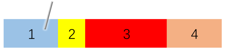
Figure 2: Sampling from a multinomial distribution, areas are proportional to the probabilities, $p(k=1)=0.25,p(k=2)=0.125,p(k=3)=0.375,p(k=4)=0.25$.

1. For $k=1,\dots,K$, compute the probabilities $p(k)$ and their sum $S=\sum_{k}p(k)$;

2. Generate a random number $u\in[0,S)$;

3. Compute the prefix sum $c_{k}=c_{k-1}+p(k)$, where $c_{0}=0$, and return the first $k$ such that $u\leq c_{k}$, with a binary search.

We refer the above procedure as the vanilla algorithm, whose time complexity is limited by step 1 and step 3, which are $O(K)$. Step 3 is a very important routine which we will use over and over again, and we refer its result as “the position of $u$ in the prefix sum array of $p(k)$” for brief.

While the vanilla algorithm is $O(K)$, the sparsity-aware algorithms li2014reducing ; zaheer2015exponential utilize the sparsity of $\bm{\mathbf{A}}$, and improve the time complexity to $O(K_{d})$, where $K_{d}$ is the average number of non-zero entries per row of $\bm{\mathbf{A}}$. The algorithm decomposes the original sampling problem as two easier sampling sub-problems. For sampling each token, it returns the result of a random sub-problem, where the probability of choosing the first sub-problem is $\frac{S}{S+Q_{v}}$, where $S=\sum_{k=1}^{K}A_{dk}\hat{B}_{vk}$ and $Q_{v}=\alpha\sum_{k=1}^{K}\hat{B}_{vk}$. The two sub-problems are defined as follows:

Problem 1

Sample $p_{1}(k)\propto A_{dk}\hat{B}_{vk}$.

This can be sampled with the vanilla algorithm we described before. But sparsity can be utilized: if $A_{dk}=0$, then $p_{1}(k)=0$ as well. Therefore, we only need to consider the indexes $k$ where $A_{dk}\neq 0$. There are only $K_{d}$ such indexes on average, therefore, the time complexity is only $O(K_{d})$ instead of $O(K)$. Similarly, $S$ can be computed in $O(K_{d})$.

Problem 2

Sample $p_{2}(k)\propto\alpha\hat{B}_{vk}\propto\hat{B}_{vk}$.

This problem is only relevant with $v$ but not $d$. We can pre-process for each $v$. There are various approaches for pre-processing which we will cover in detail in Sec. 3.2. In brief, we construct a tree $T_{v}$ for each $v$, and then each sample can be obtained with the tree in $O(\log_{W}K)$. The pre-processing step is not the bottleneck because it is done only once per iteration.

Algorithm 1 ESCA algorithm for LDA.

1:  Input: token list $L$

2:  Variable: sparse matrix $\bm{\mathbf{A}}$, dense matrix $\bm{\mathbf{B}}$ and $\bm{\mathbf{{\hat{B}}}}$, vector $Q$, sampling trees of all unique words $\bm{\mathbf{T}}$

3:  for $i\leftarrow 1\mbox{ to }\mbox{num\_iteration}$ do

4:     // E Step:

5:     for $(d,v,k)\in L$  do

6:        $k\leftarrow\mbox{Sample}(\bm{\mathbf{A}}_{d},\bm{\mathbf{\hat{B}}}_{v},Q_{v},T_{v}$)

7:     end for

8:     // M Step:

9:     $\bm{\mathbf{A}}\leftarrow\mbox{CountByDZ}(L)$

10:     $\bm{\mathbf{B}}\leftarrow\mbox{CountByVZ}(L)$

11:     $\bm{\mathbf{\hat{B}}}\leftarrow\mbox{Preprocess}(\bm{\mathbf{B}},\beta)$

12:     for $v\leftarrow 1\mbox{ {to} }V$ do

13:        $Q_{v},T_{v}\leftarrow\mbox{BuildTree}(\bm{\mathbf{\hat{B}}}_{v})$

14:     end for

15:  end for

2.4 Pseudo-Code

To make the presentation more concrete, we present the pseudocode of the ESCA algorithm as Alg. 1, which is a Bulk Synchronous Parallel (BSP) programming model. In the E-step of each iteration, all the tokens in the token list $L$ are updated independently, by calling Sample for each token. All arguments of the function Sample are read-only, and the return value is the new topic assignment $k$. In the M-step, the matrices $\bm{\mathbf{A}}$ and $\bm{\mathbf{B}}$ are calculated from the token list $L$, by functions CountByDZ and CountByVZ. Then, $\bm{\mathbf{\hat{B}}}$ is updated by the function Preprocess following Eq. (2). Finally, generate the sampling trees $T_{v}$ and sums $Q_{v}$ for each word $v$.

Algorithm 2 Sparsity aware sampling

1:  Input: sparse vector $A$, dense vector $\hat{B}$, scalar $Q$, tree $T$

2:  $S\leftarrow 0$

3:  $P\leftarrow\mbox{new sparse vector}$

4:  for  $k\leftarrow\mbox{non-zero elements of }A$ do

5:     $P_{k}\leftarrow A_{k}\times\hat{B}_{k}$

6:     $S\leftarrow S+P_{k}$

7:  end for

8:  if $\mbox{random}(0,1)<S/(S+Q)$ then

9:     $k\leftarrow$ sample from $P$

10:  else

11:     $k\leftarrow$ $T$.sample()

12:  end if

13:  return  $k$

As shown in Alg. 2, the function Sample samples the topic assignment $k$ given the rows $\bm{\mathbf{A}}_{d}$, $\bm{\mathbf{\hat{B}}}_{v}$, the sum $Q_{v}$, and the tree $T_{v}$, by implementing the sparsity-aware algorithm described in Sec. 2.3. First, we compute the probability for Problem 1, $P=\bm{\mathbf{A}}_{d}\bigodot\bm{\mathbf{\hat{B}}}_{v}$ as well as $S$, where $\bigodot$ is the element-wise product. Next, we flip a coin with the probability of head being $\frac{S}{S+Q}$. If the coin is head, perform sampling from $p_{1}(k)\propto P_{k}$, which involves finding the location of a random number in the prefix-sum array of the sparse vector $P$ as discussed in Sec. 2.3. Otherwise, sample from $p_{2}(k)\propto\hat{B}_{vk}$ with the tree $T$, which is pre-processed.

3 Design and Implementation

In this section we present SaberLDA, a high performance GPU-based system for training LDA. The design goals of SaberLDA are:

• supporting large models up to 10,000 topics;

• supporting large dataset of billions of tokens;

• providing comparable performance with a moderate size CPU cluster using a single GPU card.

It is difficult for previous GPU-based systems yan2009parallel ; zhao2015same ; tristan2015efficient to satisfy all these goals, because all of them are based on the vanilla algorithm mentioned in Sec. 2.3 which have $O(K)$ time complexity, i.e., the training time will be 100 times longer if the number of topics increase from hundreds (current) to 10,000 (goal), which is not acceptable.

To address this problem, SaberLDA adopts the sparsity-aware sampling algorithm whose time complexity is $O(K_{d})$, which is not very sensitive to the number of topics. However, exploiting sparsity is highly challenging on GPUs. The memory access is no longer sequential as that for the dense case, and the small cache size and long cache line of GPU aggravate this problem. Therefore, the memory accesses need to be organized very carefully for good locality. Moreover, vectorization is not as straightforward as the dense case since the loop length is no longer fixed and the data are not aligned, so waiting and unconcealed memory accesses can happen. Finally, updating the sparse count matrix is more complicated than dense count matrices. We now present our design of SaberLDA which addresses all the challenges.

3.1 Streaming Workflow

We first consider how to implement Alg. 1, deferring the details of the functions Sample, CountByDZ, CountByVZ, Preprocess and BuildTree to subsequent sections. The implementation involves designing the storage format, data placement (host / device), and partitioning strategies for all the data items, as well as designing the order of sampling tokens (Line 5 of Alg. 1). The data items include the token list $L$, the document-topic count matrix $\bm{\mathbf{A}}$, the word-topic count matrix $\bm{\mathbf{B}}$, and the word-topic distribution matrix $\bm{\mathbf{\hat{B}}}$.

The aforementioned design should maximize the locality, and meanwhile, keep the size of the data items within the budget of GPU memory even when both $K$ and the data size are large. This is challenging because locality emerges as a new design goal to support sparsity-aware algorithms, while previous dense matrix based GPU systems yan2009parallel ; zhao2015same ; tristan2015efficient only have one goal (i.e., fitting into the memory budget) instead of the two which need to be obtained simultaneously in our method. As we will see soon, the simple data layout in previous systems such as sorting all tokens by document-id yan2009parallel ; zhao2015same ; tristan2015efficient ; zaheer2015exponential or by word-id yu2015scalable cannot satisfy both requirements, and we will propose a hybrid data layout to address this problem.

3.1.1 Storage Format

We analyze the access pattern of these data items described in Alg. 1 and Alg. 2. The token list $L$ is accessed sequentially, and we store it with an array. The document-topic count matrix $\bm{\mathbf{A}}$ is accessed by row, and the Sample function iterates over its non-zero entries, so we store it by the compressed sparse rows (CSR) format to avoid enumerating over zero entries. Besides efficiency, the CSR format also reduces the memory consumption and host/device data transferring time comparing with the dense matrix format in previous implementations yan2009parallel ; zhao2015same ; tristan2015efficient . The word-topic matrices $\bm{\mathbf{B}}$ and $\bm{\mathbf{\hat{B}}}$ are randomly accessed, and we store them as dense matrices. Table 2 lists the memory consumption of each data item in the PubMed dataset (See Sec. 4 for the details), where we can observe that representing $\bm{\mathbf{A}}$ as sparse matrix indeed saves a lot of memory when $K\geq 1,000$, and the GPU memory is large enough to hold $\bm{\mathbf{B}}$ and $\bm{\mathbf{\hat{B}}}$ for the desired number of topics.

Table 2: Memory Consumption of PubMed Dataset

Data	Word-Topic Matrix $\bm{\mathbf{B}}$, $\bm{\mathbf{\hat{B}}}$	Token List $L$	Doc-Topic Matrix $\bm{\mathbf{A}}$
			Dense	Sparse
K	V=141k	T=738M	D=8.2M
100	0.108 GB	8.65 GB	3.2 GB	5.8 GB
1k	1.08 GB	8.65 GB	32 GB	5.8 GB
10k	10.8 GB	8.65 GB	320 GB	5.8 GB

3.1.2 Data Placement and Partitioning Strategy

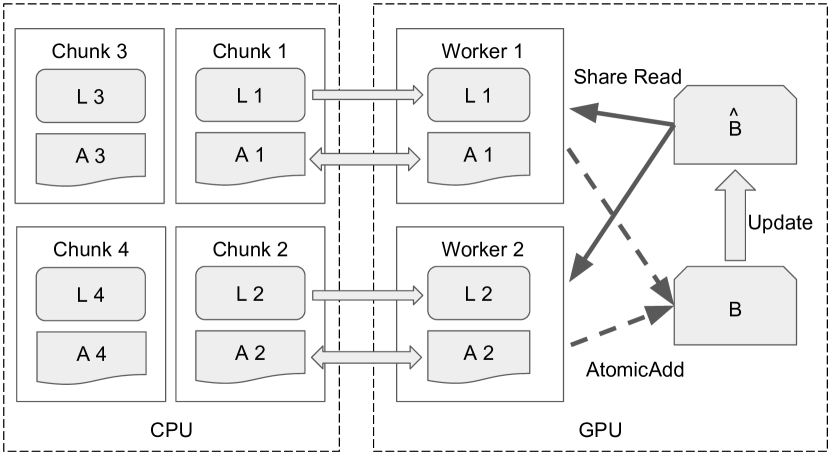
Figure 3: Streaming workflow of SaberLDA. $\bm{\mathbf{L}}$: Token List, $\bm{\mathbf{A}}$: document-topic count matrix, $\bm{\mathbf{B}}$: word-topic count matrix, $\bm{\mathbf{\hat{B}}}$: word-topic probability matrix.

However, the token list $L$ and the document-topic matrix $\bm{\mathbf{A}}$ cannot fit in the GPU memory, because the $L$ grows linearly with the number of tokens, and the size of $\bm{\mathbf{A}}$ grows linearly with the number of documents. Therefore, the sizes of both data items grow rapidly with the size of the dataset. Since one of our major design goals is to support large datasets with billions of tokens, $L$ and $\bm{\mathbf{A}}$ cannot be held in GPU memory because they can be arbitarily large as the size of the dataset grows.

To address this problem, we treat $L$ and $\bm{\mathbf{A}}$ as streams: we store them in the main memory, partition them into chunks, and process a few chunks with the GPU at a time. We partition $L$ and $\bm{\mathbf{A}}$ by document, i.e., each chunk has all tokens from a certain set of documents along with the corresponding rows of $\bm{\mathbf{A}}$. Several workers are responsible of performing the sampling (Alg. 2) for the tokens in each chunk, as illustrated in Fig. 3. Each worker is a cudaStream that fetches a chunk from the main memory, samples the topic assignments for all the tokens in that chunk, updates the document-topic count maxis $\bm{\mathbf{A}}$, and sends the updated $\bm{\mathbf{A}}$ back to the main memory. The computation and communication are overlapped by having multiple workers. The word-topic matrices $\bm{\mathbf{B}}$ and $\bm{\mathbf{\hat{B}}}$ are in the GPU memory, while in the sampling stage, all the workers read $\bm{\mathbf{\hat{B}}}$ and updates $\bm{\mathbf{B}}$. When the sampling of each iteration is finished, $\bm{\mathbf{\hat{B}}}$ is updated with $\bm{\mathbf{B}}$.

3.1.3 Order of Sampling Tokens

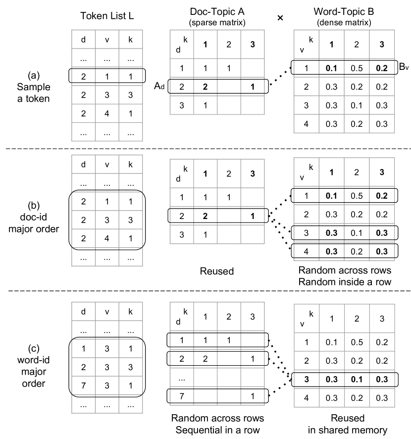
Figure 4: Memory Access Pattern of Sampling.

We now discuss the order of sampling tokens, i.e., executing Sample for each token in Alg. 1. Although theoretically these tokens can be sampled in any order, the ordering greatly impacts the locality, as we shall see soon; therefore calling for a careful treatment.

As illustrated as Fig. 4(a), sampling $k$ for a token $(d,v,k)$ requires evaluating a element-wise product of two rows (Line 4-7 of Alg. 2), i.e., the $d$-th row of the document-topic count matrix $\bm{\mathbf{A}}_{d}$ and the $v$-th row of the word-topic probability matrix $\bm{\mathbf{\hat{B}}}_{v}$. The element-wise product involves accessing all non-zero entries of $\bm{\mathbf{A}}_{d}$ (sequential), and accessing the elements of $\bm{\mathbf{\hat{B}}}_{v}$ indexed by the non-zero entries of $\bm{\mathbf{A}}_{d}$ (random).

There are two particular visiting orders which reuse the result of previous memory accesses for better locality. The doc-major order sorts the tokens by their document-id’s, so that the tokens belonging to the same document are adjacent in the token list. Before processing the tokens in the $d$-th document, the row $\bm{\mathbf{A}}_{d}$ can be fetched into the shared memory and reused for sampling all the subsequent tokens in that document. On the other hand, the access of $\bm{\mathbf{\hat{B}}}_{v}$ cannot be reused, because each token requires to access random elements (indexed by the non-zero entries of $\bm{\mathbf{A}}_{d}$) in random row of the word-topic count matrix $\bm{\mathbf{\hat{B}}}$, as shown in Fig. 4 (b). The bottleneck of this approach is accessing $\bm{\mathbf{\hat{B}}}$, where both the row index and column index are random.

On the contrary, the word-major order sorts the tokens by their word-id’s, so that the tokens belong to same word are adjacent in the token list. Before processing the tokens of the $v$-th word, the row $\bm{\mathbf{\hat{B}}}_{v}$ can be fetched into the shared memory and reused for sampling all the subsequent tokens of that word. Each token needs to access all the elements of a random row $\bm{\mathbf{A}}_{d}$ (Fig. 4 (c)). The bottleneck of this approach is accessing $\bm{\mathbf{A}}$, where only the row index is random.

The memory hierarchies are quite different on CPUs and GPUs. CPUs have larger cache size ($>$30MB) and shorter cache line (64B), while GPUs have smaller cache size ($>$2MB) and longer cache line. On CPUs, when $K$ and $V$ are small, the document-major order can have better cache locality than the word-major order because $\bm{\mathbf{\hat{B}}}$ can fit in cache zaheer2015exponential . But for GPUs, the word-major order has clear advantage that it efficiently utilizes of the cache line by accessing whole rows of $\bm{\mathbf{A}}_{d}$ instead of random elements. Therefore, we choose the word-major order for SaberLDA.

3.1.4 Partition-by-Document and Order-by-Word

Putting all the above analysis together, SaberLDA adopts a hybrid data layout called partition-by-document and order-by-word (PDOW), which means to firstly partition the token list by document-id, and then sort the tokens within each chunk by word-id. Unlike the simple layouts such as sorting all tokens by document-id or by word-id in previous systems yan2009parallel ; zhao2015same ; tristan2015efficient ; zaheer2015exponential ; yuan2014lightlda ; yu2015scalable , PDOW combines the advantages of both by-document partitioning and word-major ordering, and simultaneously improves cache locality with the word-major order, and keeps the GPU memory consumption small with the by-document partitioning.

The number of chunks presents a tradeoff between memory consumption and locality. The memory consumption is inversely proportional to the number of chunks, but the number of times to load each row of $\bm{\mathbf{B}}$ into shared memory is proportional to the number of chunks. The chunk size should not be too small to ensure good locality, i.e., the pre-loaded $\bm{\mathbf{B}}_{v}$ should be reused for a suffciently large number of times. In SaberLDA, we minimize the number of chunks as long as the memory is sufficient.

3.2 Warp-based Sampling

⬇

int WarpSample(SparseVector A, __shared__ DenseVector B_hat, Wary_tree T, RandomSeed &seed) {

float S = 0;

__shared__ float P[A.size()];

for (int i=thread_id; i<A.size(); i+=32) {

int k = A[i].idx;

P[i] = A[i].val * B_hat[k];

S += P[i];

}

S = warp_sum(S);

if (RandomFloat(seed) < S/(S+T.sum())) {

float x = RandomFloat(seed) * S;

float ps = 0;

for (int i=0; i<A.size(); i+=32) {

ps += warp_prefix_sum(P[i+thread_id]);

int vote_id = warp_vote(ps >= x);

if (vote_id != -1)

return A[i+vote_id].idx;

ps = warp_copy(ps, 31);

}

} else return T.Sample(seed);

}

Figure 5: Warp-based sampling kernel.

We now turn to the Sample function (Alg. 2), which is the most time consuming part of LDA. To understand the challenges and efficiency-related considerations, it is helpful to have a brief review of GPU architecture.

GPUs follow a single instruction multiple data (SIMD) pattern, where the basic SIMD unit is warp, which has 32 data lanes. Each lane has its own ALU and registers, and all the lanes in a warp execute the same instruction. In CUDA, each thread is executed on a lane, and every adjacent 32 threads share the same instruction. Readers can make an analogy between GPU warp instruction and CPU vector instruction.

The most straightforward implementation of sampling on GPU is thread-based sampling, which samples each token with a GPU thread. Therefore, 32 tokens are processed in parallel with a warp. Thread-based sampling is acceptable when $\bm{\mathbf{A}}$ is dense because the loop length (Line 4 of Alg. 2) is always $K$, and are no branches (Line 8 of Alg. 2). However, this approach has several disadvantages when $\bm{\mathbf{A}}$ becomes sparse. Firstly, because each token corresponds to different rows of $\bm{\mathbf{A}}$, the loop length of each thread are different (Line 4 of Alg. 2). In this case, all the threads need to wait until the longest loop is finished, introducing long waiting time. Secondly, there are branches in the sampling procedure, for example, the branch choosing which distribution to sample (Line 8 of Alg. 2). The branches cause the thread divergence problem, i.e., if some of the threads go to one branch and other threads go to another branch, the warp need to perform the instructions of both branches, which again increases the waiting time. Finally, the access to $\bm{\mathbf{A}}$ is unconcealed (Line 5 of Alg. 2) because the threads are accessing different and discontinuous addresses of the global memory.

To overcome the disadvantages of thread-based sampling, SaberLDA adopts warp-based sampling, where all the threads in a warp collaboratively sample a single token. However, there are also challenges for warp-based sampling — all the operations need to be vectorized to maximize the performance.

We now present our vectorized implementation. As mentioned in Sec. 2.4, the sampling involves computing the element-wise product (Line 4-7 of Alg. 2), randomly decide which branch to sample (Line 8 of Alg. 2), and depending on which branch is chosen, sample from $P$ (Line 9 of Alg. 2), or sample with the pre-processed tree (Line 11 of Alg. 2). Before starting the presentation, we also remind the readers that $\bm{\mathbf{A}}$ is in global memory, and all the other data items such as $\bm{\mathbf{B}}_{v}$ and $T_{v}$ are pre-loaded into shared memory taking advantage of PDOW as discussed in Sec. 3.1.3.

3.2.1 Element-wise Product

The element-wise product step is vectorizable by simply letting each thread process an index and a warp compute the element-wise product for 32 indices at a time. All the threads are efficiently utilized except for the last 32 indices if the number of non-zero entries of Ad is not a multiple of 32. The waste is very small since the number of non-zero entries is typically much larger than 32, e.g., 100.

3.2.2 Choosing the Branch

This step only consists a random number generation and a comparison, whose costs are negligible. Note that thread divergence will not occur as for the thread-based sampling since the whole warp goes to one branch or the other.

3.2.3 Sample from $P$

This step consists of the three steps mentioned in Sec. 2.3, where the element-wise product is already computed. We need to generate a random number, and find its position in the prefix-sum array of $P$.

Firstly, we need to vectorize the computation of the prefix sum, i.e., computing the prefix sum of 32 numbers using 32 threads. Because of the data dependency, the prefix sum cannot be computed with a single instruction. Instead, __shuf_down operations are required, and the prefix sum can be computed in $O(\log_{2}32)$ instructions prefixsum . We refer this routine as warp_prefix_sum. Given the prefix sum, we need to figure out the index of the first element which is greater than or equal to the value. This can be achieved in two steps:

1. The warp-vote intrinsic __ballot forms a 32-bit integer, where the $i$-th bit is one if the $i$-th prefix sum is greater than or equal to the given value ballot ,

2. The __ffs intrinsic returns the index of the first bit 1 of a 32-bit integer,

where we refer these two steps as warp_vote, which returns an index that is greater than or equal to the given value, or -1 if there is no such index.

Deferring the discussion for the pre-processed sampling for a while, Fig. 5 is an example code of our vectorized warp-based sampling, where we omit some details such as whether the vector length is a multiple of the warp size, and the warp_copy(a, id) function returns $a$ on the thread $id$. There is no waiting or thread divergence issue as discussed above.

Besides the eliminated waiting time and thread divergence, the memory access behavior of our implementation is good as well. For the element-wise product, the access to $\bm{\mathbf{A}}$ is continuous. More specifically, the warp accesses two 128-byte cache lines from the global memory, and each thread consumes two 32-bit numbers (an integer index and a float32 value). The accesses to $\bm{\mathbf{B}}$ are random, but they are still efficient since the current row $\bm{\mathbf{B}}_{v}$ is in shared memory. All the rest operations only access data items in the shared memory, e.g., $P$.

3.2.4 $W$-ary Sampling Tree

⬇

struct Wary_tree {

float L1, L2;

__shared__ Array L3, L4;

Wary_tree(Array p)

{

L4.Alloc(p.size())

L4 = array_prefix_sum(p);

L3.Alloc(L4.size()/32)

for (int i = thread_id; i<L3.size() ; i += 32)

L3[i] = L4[i*32-1];

L2 = L3[thread_id*32-1];

L1 = warp_copy(L2, 31);

}

float Sum() { return L1; }

int Sample(RandomSeed &seed)

{

float x = RandomFloat(seed) * L1;

int off3 = warp_vote(L2 >= x) * 32;

int off4 = (off3 + warp_vote(L3[off3+thread_id] >= x))*32;

return off4 + warp_vote(L4[off4+thread_id]>=x);

}

};

Figure 6: W-ary Sampling Tree.

We now present the deferred details of the pre-processed sampling (Line 11 of Alg. 2). The pre-processed sampling is new in sparsity-aware algorithms, since the vanilla algorithm does not break the original sampling problem into sub-problems. Therefore, previous GPU-based systems do not have this problem. As discussed in Sec. 2.3, the pre-processed sampling problem is essentially the same problem as sampling from $P$, but there are only $V$ different sampling problems, so we can pre-process for each problem to accelerate this process. In previous literature, there are two main data structures for that problem, and we briefly review them.

• An alias table walker1977efficient can be built in $O(K)$ time, and each sample can be obtained in $O(1)$ time afterwards. However, building the alias table is sequential;

• A Fenwick tree yu2015scalable can be built in $O(K)$ time, and each sample can be obtained in $O(\log_{2}K)$ time afterwards. However, the branching factor of the Fenwick tree is only two, so the 32-thread GPU warp cannot be fully utilized.

Both approaches are designed for CPU, and are slow to construct on GPU because they cannot be vectorized. Vectorization is critical because using only one thread for pre-processing can be much slower than using a full warp for pre-processing. To allow vectorized pre-processing, we propose a $W$-arytree, which can be constructed in $O(K)$ time with full utilization of GPU warp. Subsequent samples can be obtained in $O(\log_{W}K)$ time, where $W$ is the number of threads in a GPU warp, i.e., 32.

We emphasize that our main focus is on the efficient construction of the tree instead of efficient sampling using the tree, because the cost of sampling using the tree is negligible comparing with sampling from $P$. Moreover, the sampling using our $W$-arytree is efficient anyway because $K$ is in the order of 10,000, and $\log_{W}K=4$, so $O(\log_{W}K)=O(4)$ is at the same level of the $O(1)$ alias table algorithm.

Our $W$-arytree is designed for efficiently finding the location of a given number in the prefix-sum array. Each node of the tree stores a number, where the bottom-most level nodes store the prefix-sums of the given array. The length of an upper level is equal to the length of the lower level divided by $W$, and the $i$-th node in an upper level is equal to the $iW-1$ node in the lower level. Constructing the tree is illustrated in Fig. 7. This procedure is efficient because all the nodes in one layer can be constructed in parallel. Therefore, the GPU warp can be efficiently utilized with the warp_prefix_sum function we mentioned before, which uses $W$ threads to compute the prefix-sum of $W$ numbers in parallel.

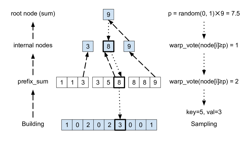
Figure 7: Building a 3-ary tree and sampling from the tree.

To find the position of a given value in the prefix-sum array, we recursively find the position at each level, from top to bottom (Fig. 7). Based on the particular construction of our tree, if the position on the $l$-th level is $i$, then the position at the $l+1$-th level is between $iW$ and $iW+W-1$. Therefore, only $W$ nodes need to be checked on each level. This checking can be done efficiently using the warp_vote function we mentioned before, and the memory access is efficient because the tree is stored in the shared memory (Sec. 3.1.3), and it only needs to read $W$ continuous floating point numbers, i.e., a 128-byte cache line for each level.

The amount of memory accesses can be further reduced. We use a four-level tree for SaberLDA, which supports up to $W^{3}=32,768$ topics. The first and second layers contain only 1 and 32 nodes, respectively, and they can be stored in the thread registers. In this way, only two shared memory cache lines for level 3 and 4 are accessed per query. Fig. 6 is the code for the $W$-arytree.

3.3 Efficient Count Matrix Update

Finally, we discuss how to efficiently update the count matrices $\bm{\mathbf{A}}$ and $\bm{\mathbf{B}}$. When the sampling of all tokens with the same word is finished, the corresponding row $\bm{\mathbf{B}}_{v}$ of the word-topic count matrix is ready to be updated. The atomicAdd function must be used because there may be multiple workers updating the same row, but the overhead is very low since the time complexity of updating is lower than the time complexity of sampling. The word-topic probability matrix $\bm{\mathbf{\hat{B}}}$ can be easily generated according to Eq. (2) from $\bm{\mathbf{B}}$ after all the updates of the latter are finished. Maximal parallel performance can be achieved since both matrices are dense.

Figure 8: An example for segmented count

However, the update of the document-topic matrix $\bm{\mathbf{A}}$ is challenging since $\bm{\mathbf{A}}$ is sparse. To update an entry of a sparse matrix, one must find the location of that entry, which is difficult to vectorize. Therefore, instead of updating, we rebuild the count $\bm{\mathbf{A}}$ after the sampling of each partition is finished.

A naïve approach of rebuilding the count matrix is to sort all the tokens by first document-id $d$ then topic assignment $k$, and perform a linear scan afterwards. However, the sorting is expensive since it requires to access the global memory frequently. Moreover, the efficiency of sorting decreases as the chunk size increases.

We propose a procedure called shuffle and segmented count (SSC) to address this problem. To rebuild the count matrix, we first perform a shuffle to organize the token list by the document-id’s, i.e., segment the token list as smaller lists where the tokens in each list share the same document-id. Since the document-id’s of the tokens are fixed, the shuffle can be accelerated with a pre-processed pointer array, which points each token to its position in the shuffled list. Therefore, to perform shuffling, we only need to place each token according to the pointers. Furthermore, we can reduce the accesses to global memory by creating the counts for each smaller token list individually, where these token lists are small enough to fit in the shared memory.

Creating the counts is a common problem as known as segmented count, which means for segmenting the tokens by $d$ and counting $k$ in each segment. Unlike similar problems such as segmented sort segsort and segmented reduce segreduce which have fully optimized algorithms for GPUs, efficient GPU solution of segmented count is not well studied yet.

We propose a solution of segmented count which is sufficiently efficient for SaberLDA. Our procedure consists of three steps, as illustrated in Fig. 8:

1. Perform a radix sort by $k$ in shared memory;

2. Calculate the prefix sum of the adjacent difference, in order to get the number of different topics and the order number of each topic;

3. Assign the topic number at corresponding order number, and increase the counter of the same topic.

3.4 Implementation Details and Load Balancing

In SaberLDA, a word and a token are processed with a a block and a warp, respectively. Each block has its own shared memory to hold the rows $\bm{\mathbf{\hat{B}}}_{v}$ and $\bm{\mathbf{B}}_{v}$, where the former is fetched from the global memory before sampling any tokens in the current word $v$ and the latter is written back to global memory after the sampling. To minimize the number of memory transactions, we also align the memory address of each row of $\bm{\mathbf{A}}$ by 128 bytes.

The workload for each block is determined by the size of its chunk, the workload for each block is determined by the number of tokens in the word, and the workload for each warp is determined by the number of non-zero entries in the document. To minimize the imbalance of the workload, we apply dynamic scheduling at all the three levels, i.e., a block fetches a new word to process when it is idle, and similarly, a warp fetches a new token to process when it is idle.

Because the term frequency of a natural corpus often follows the power law kingsley1932selective , there are a few high-frequency words which have much more tokens than other low-frequency words. Therefore, the block level workload is more imbalanced than the other two levels. To address this problem, we further sort the words decreasingly by the number of tokens in it, so that the words with most number of tokens will be executed first, and then the words with small number of tokens are executed to fill the imbalance gaps.

4 Evaluation

Table 3: Statistics of various datasets, where $T$ is the total number of words in the corpus.

Dataset	$D$	$T$	$V$	$T/D$
NYTimes  asuncion2007uci	300K	100M	102k	332
PubMed  asuncion2007uci	8.2M	738M	141k	90
ClueWeb12 subset	19.4M	7.1B	100k	365

In this section, we provide extensive experiments to analyze the performance of SaberLDA, and compare SaberLDA with other cutting-edge open source implementations on various widely adopted datasets listed in Table 3.

The code of SaberLDA is about 3,000 lines, written in CUDA and C++, and compiled with NVIDIA nvcc 8.0 and Intel ICC 2016. Our testing machine has two Intel E5-2670v3 CPUs, with 12 cores each CPU, 128 GB main memory and a NVIDIA GTX 1080 GPU.

The hyper-parameters $\alpha=50/K$ and $\beta=0.01$ are set according to previous works yao2009efficient ; li2014reducing ; yu2015scalable ; chen2016warplda .

The training time of LDA depends on both the number of iterations to converge and the time for each iteration. The former depends on the algorithm, e.g., variational Bayes algorithm blei2003latent typically requires fewer iterations than ESCA zaheer2015exponential to converge. The latter depends on the time complexity of sampling each token as well as the implementation, e.g., the sparsity-aware algorithm has $O(K_{d})$ time complexity and performs faster than the $O(K)$ vanilla algorithms. Therefore, we use various metrics to compare LDA implementations:

• We use time per iteration or throughput to compare different implementations of the same algorithm, e.g., compare SaberLDA, which is a GPU implementation of the ESCA algorithm, with a CPU implementation of the same algorithm, because they require the same number of iterations to converge. The throughput is defined as the number of processed tokens divided by the running time, and the unit is million tokens per second (Mtoken/s).

• Since different algorithms require different numbers of iterations to converge, the time per iteration metric is no longer informative. Therefore, we compare different algorithms by the required time to converge to a certain model quality. The model quality is assessed by holdout log-likelihood per token, using the partially-observed document approach  wallach2009evaluation . Higher log-likelihood indicates better model quality.

4.1 Impact of Optimizations

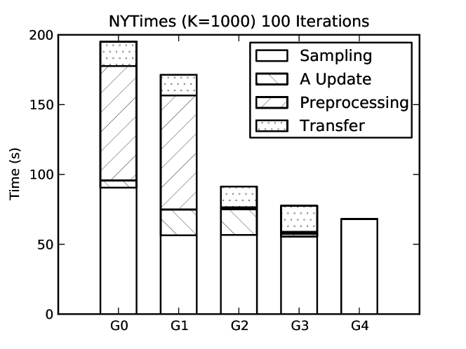
Figure 9: Impact of optimizations. G0: Baseline; G1: PDOW; G2: $W$-arytree; G3: SSC; G4: Asynchronous.

We first investigate the impact of each optimization technique we proposed in Sec. 3, by training LDA on the NYTimes dataset with 1,000 topics for 100 iterations. The results are shown in Fig. 9, where the total elapsed time is decomposed as the Sample function, rebuilding document-topic matrix $\bm{\mathbf{A}}$, constructing pre-processed data structures for sampling (pre-processing), and data transferring between CPU and GPU.

G0 is the most straightforward sparsity-aware implementation on GPU which sorts all tokens by documents, performs the pre-processed sampling with the alias table, and builds count matrices by naïve sorting of all tokens. G1 adopts the PDOW strategy proposed in Sec. 3.1.4, and the time of sampling is reduced by almost 40% because of the improved locality for sampling. Note rebuilding the doc-topic matrix A takes more time in G1 than in G0, because the tokens are ordered by word, and the sorting becomes slower.

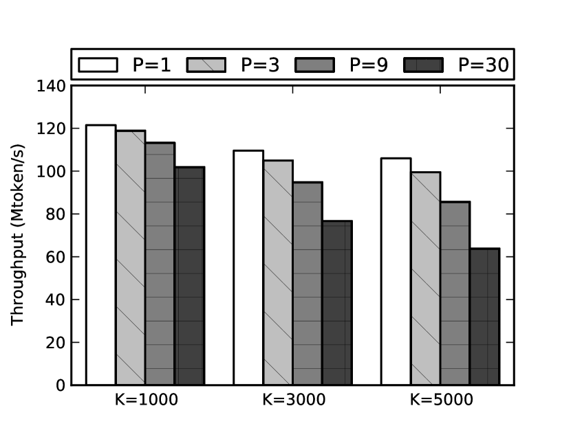
(a)

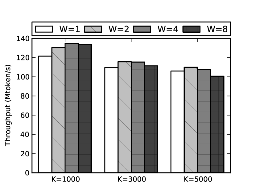
(b)

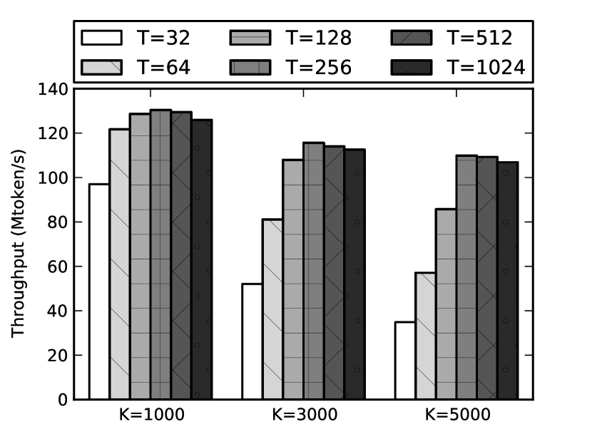
(c)

Figure 10: Dateset: NYTimes. (a) Performance of different number of partitions. (b) Performance of different number of workers. (c) Performance of different number of threads.

The bottleneck of G1 is the construction of the alias table, which is hard to vectorize. In G2, we replace the alias table with the $W$-arytree, which fully utilizes warps to greatly reduce the construction time by 98%.

Then, we optimize the rebuilding of the document-topic matrix $\bm{\mathbf{A}}$ with SSC (Sec. 3.3), which reduces the rebuilding time by 89%. Up to now, the time for updating $\bm{\mathbf{A}}$ and pre-processing is neglectable.

Finally, in G4, we enable multiple workers running asynchronously to hide the data transfer between CPU and GPU. It reduce 12.3% of total running time in this case. Overall, all these optimizations achieve 2.9x speedup comparing with the baseline version G0. We emphasize that even G0 is already highly optimized, and should handle more topics than previous GPU implementations because it still adopts the sparsity-aware algorithm whose time complexity is$O(K_{d})$.

4.2 Performance Tuning

Table 4: Memory bandwidth utilization, NYTimes, $K=1000$.

	Throughput (GB/s)	Utilization
Global memory	144	50%
L2 cache	203	30%
L1 unified cache	894	20%
Shared memory	458	20%

Tuning parameters, such as the number of workers, the number of chunks and the number of threads in a CUDA kernel can largely affect the performance. In order to fully understand the impact of tuning parameters, we analyze the performance of SaberLDA under different parameter settings. We evaluate the total running time of the first 100 iterations on the NYTimes dataset with the number of topics varying from 1,000, to 3,000, and to 5,000.

4.2.1 Number of Chunks

Firstly, we analyze the single worker performance with various numbers of partitions, as shown in Figure 10 (a). We can see that the performance degrades with more partitions because of the degraded locality, but partitioning is necessary when the dataset is too large to be held in GPU. We keep the number of partitions as small as possible to maximize the performance.

4.2.2 Number of Workers

Figure 10 (b) presents the performance with different numbers of workers. We fix the number of chunks to 10. Using multiple workers can hide the data transfer time between GPU and CPU, and reduce the overall time consumption. We observe a 10% to 15% speedup from single worker to 4 workers, where the speedup is quite close to the proportion of data transferring shown in Fig. 9.

4.2.3 Number of Threads

Tuning the number of threads in each block maximizes the system performance. For the kernel function, more threads imply fewer active blocks, which reduces the total shared memory usage in a multiprocessor, but increases the in-block synchronization overhead of warps. Figure 10 (c) shows that setting 256 threads in a block always achieves the best performance for various numbers of topics.

4.3 Profiling Analysis

Next, we analyze the utilization of hardware resources with NVIDIA visual profiler. We focus on memory bandwidth because LDA is a memory intensive task chen2016warplda .

Table 4 is the memory bandwidth utilization of the first 10 iterations on NYTimes with $K=1,000$. Statistics show that the throughput accessing global memory reaches more than 140 GB/s, which is about 50% of the bandwidth. This shows clear advantage over CPUs, given that the bandwidth between main memory and CPU is only 40 to 80 GB/s. The throughput of the L2 cache, unified L1 cache and shared memory is 203GB/s, 894GB/s and 458GB/s respectively, while the utilization is lower than 25%. Therefore, these are not the bottleneck of the overall system performance.

We further use performance counters to examine of kernel function. The memory dependency is the main reason of instruction stall (47%), and the second reason is execution dependency (27%). The hotspot is computing the element-wise product between sparse vector $\bm{\mathbf{A}}_{d}$ and dense vector $\bm{\mathbf{\hat{B}}}_{w}$, which is expected because it accesses global memory.

4.4 Comparing with Other Implementations

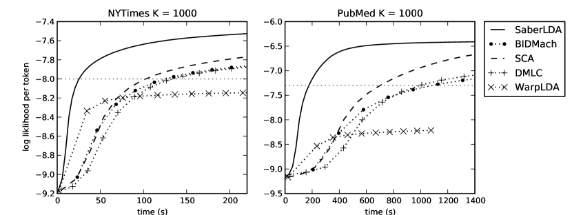
Figure 11: Convergence over time with 1000 topics. The left is evaluated on the NYTimes dataset, while the right is on the PubMed dataset.

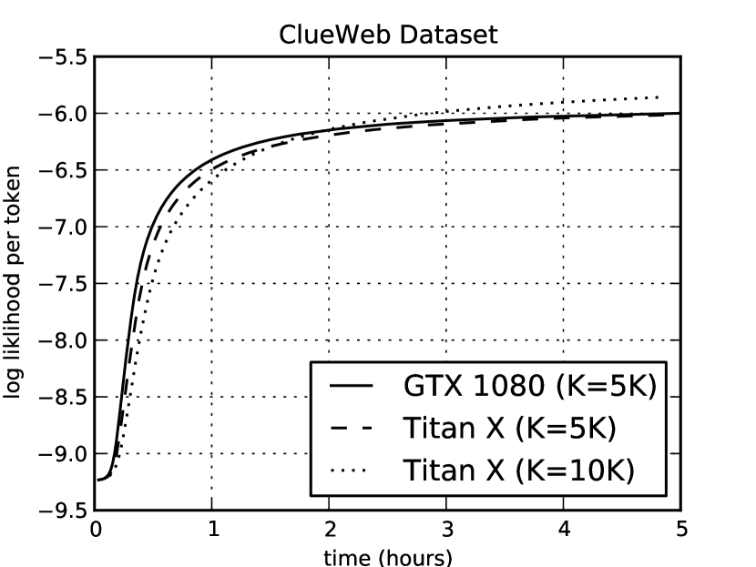
Figure 12: The convergence of SaberLDA on ClueWeb Subset.

We compare SaberLDA with a state-of-the-art GPU-based implementation BIDMach zhao2015same as well as three state-of-the-art CPU-based methods, including ESCA (CPU), DMLC dmlclda and WarpLDA chen2016warplda . BIDMach zhao2015same is the only open-sourced GPU-based method. BIDMach reports better performance than Yan et. al’s mehtod zhao2015same ; yan2009parallel , and Steele and Tristan’s method only reports tens of topics in their paper. Therefore, BIDMach is a strong competitor. ESCA (CPU) is a carefully optimized CPU version of the ESCA algorithm which SaberLDA also adopts. DMLC has various multi-thread LDA algorithms on CPU, and we choose its best performing FTreeLDA. WarpLDA is a state-of-art distributed LDA implementation on CPU based on the Metropolis-Hastings algorithm, and uses a cache-efficient $O(1)$ sampling algorithm to obtain high per-iteration throughput.

We compare the time to converge of these implementations on NYTimes and PubMed datasets, with the number of topics $K=1,000$. Figure 12 shows the convergence over time. We compare the time to converge to the per-token log-likelihood of $-8.0$ and $-7.3$, for NYTimes and PubMed, respectively. SaberLDA is about 5.6 times faster than BIDMach. We also attempt to perform the comparison with 3,000 and 5,000 topics, and find that BIDMach is more than 10 times slower than SaberLDA with 3,000 topics, and reports an out-of-memory error with 5,000 topics. This is as expected because the time consumption of BIDMach grows linearly with respect to the number of topics, and its dense matrix format is much more memory consuming than SaberLDA.

Finally, SaberLDA is about 4 times faster than ESCA (CPU) and 5.4 times faster than DMLC on the two datasets with $K=1,000$, where WarpLDA converges to a worse local optimum possibly because of its inexact Metropolis-Hastings step and the different metric with its paperr chen2016warplda which we use to assess model quality. This shows that SaberLDA is more efficient than CPU-based implementations.

4.5 A Large Dataset

Finally, to demonstrate the ability of SaberLDA to process large datasets, we test the performance of SaberLDA on a large subset of the ClueWeb dataset, which is a crawl of webpages.  We filter out the stop words and keep the remaining 100,000 most frequent words as our vocabulary, which is comparable to the vocabulary size of NYTimes. We use the entire CPU memory to hold as many documents as possible, which is 19.4 million, and the total number of tokens is 7.1 billion, which is about 10 times larger than the PubMed dataset.

In this experiment, we also use GTX Titan X (Maxwell), which has 12GB global memory besides GTX 1080, which has 8GB global memory. We compare the performance of GTX 1080 and Titan X with 5,000 topics.

The algorithm convergences in 5 hours on both cards, where the throughput of GTX 1080 is 135 Mtoken/s and the throughput of Titan X is 116 Mtoken/s. With 10,000 tokens, it also convergences in 5 hours with a throughput of 92 Mtoken/s.

5 Conclusions

We present SaberLDA, a high performance sparsity-aware LDA system on GPU. Adopting sparsity-aware algorithms, SaberLDA overcomes the problem of previous GPU-based systems, which support only a small number of topics. We propose novel data layout, warp-based sampling kernel, and efficient sparse count matrix updating algorithm to address the challenges induced by sparsity, and demonstrate the power of SaberLDA with extensive experiments. It can efficiently handle large-scale datasets with up to 7 billion tokens and learn large LDA models with up to 10,000 topics, which are out of reach for the existing GPU-based LDA systems.

In the future, we plan to extend SaberLDA to multiple GPUs and machines. Developing algorithms that converge faster and enjoy better locality is also our future work.

References

- [1] Amr Ahmed, Moahmed Aly, Joseph Gonzalez, Shravan Narayanamurthy, and Alexander J Smola. Scalable inference in latent variable models. In Proceedings of the fifth ACM international conference on Web search and data mining, pages 123–132. ACM, 2012.
- [2] Arthur Asuncion and David Newman. Uci machine learning repository, 2007.
- [3] David M Blei, Andrew Y Ng, and Michael I Jordan. Latent dirichlet allocation. JMLR, 3:993–1022, 2003.
- [4] Jordan L Boyd-Graber, David M Blei, and Xiaojin Zhu. A topic model for word sense disambiguation. In EMNLP-CoNLL, 2007.
- [5] Liangliang Cao and Li Fei-Fei. Spatially coherent latent topic model for concurrent segmentation and classification of objects and scenes. In ICCV, 2007.
- [6] J. Chang and D. Blei. Relational topic models for document networks. In AISTATS, 2009.
- [7] Jianfei Chen, Kaiwei Li, Jun Zhu, and Wenguang Chen. Warplda: a cache efficient o (1) algorithm for latent dirichlet allocation. In VLDB, 2016.
- [8] Wen-Yen Chen, Jon-Chyuan Chu, Junyi Luan, Hongjie Bai, Yi Wang, and Edward Y Chang. Collaborative filtering for orkut communities: discovery of user latent behavior. In WWW, 2009.
- [9] Thomas L Griffiths and Mark Steyvers. Finding scientific topics. Proceedings of the National academy of Sciences, 101(suppl 1):5228–5235, 2004.
- [10] Tomoharu Iwata, Takeshi Yamada, and Naonori Ueda. Probabilistic latent semantic visualization: topic model for visualizing documents. In KDD, 2008.
- [11] Zipf George Kingsley. Selective studies and the principle of relative frequency in language, 1932.
- [12] Aaron Q Li, Amr Ahmed, Sujith Ravi, and Alexander J Smola. Reducing the sampling complexity of topic models. In KDD, 2014.
- [13] John D. Owens Mark Harris, Shubhabrata Sengupta. Parallel prefix sum (scan) with cuda. http://http.developer.nvidia.com/GPUGems3/gpugems3_ch39.html, 2007.
- [14] NVIDIA. Segmented reduction. https://nvlabs.github.io/moderngpu/segreduce.html, 2013.
- [15] NVIDIA. Segmented sort and locality sort. https://nvlabs.github.io/moderngpu/segsort.html, 2013.
- [16] NVIDIA. Cuda c programming guide. http://docs.nvidia.com/cuda/cuda-c-programming-guide/index.html#warp-vote-functions, 2015.
- [17] Jean-Baptiste Tristan, Joseph Tassarotti, and Guy Steele. Efficient training of lda on a gpu by mean-for-mode estimation. In Proceedings of the 32nd International Conference on Machine Learning (ICML-15), pages 59–68, 2015.
- [18] Alastair J Walker. An efficient method for generating discrete random variables with general distributions. ACM Transactions on Mathematical Software (TOMS), 3(3):253–256, 1977.
- [19] Hanna M Wallach, Iain Murray, Ruslan Salakhutdinov, and David Mimno. Evaluation methods for topic models. In Proceedings of the 26th Annual International Conference on Machine Learning, pages 1105–1112. ACM, 2009.
- [20] Yi Wang, Xuemin Zhao, Zhenlong Sun, Hao Yan, Lifeng Wang, Zhihui Jin, Liubin Wang, Yang Gao, Jia Zeng, Qiang Yang, et al. Towards topic modeling for big data. ACM Transactions on Intelligent Systems and Technology, 2014.
- [21] Feng Yan, Ningyi Xu, and Yuan Qi. Parallel inference for latent dirichlet allocation on graphics processing units. In Advances in Neural Information Processing Systems, pages 2134–2142, 2009.
- [22] Limin Yao, David Mimno, and Andrew McCallum. Efficient methods for topic model inference on streaming document collections. In Proceedings of the 15th ACM SIGKDD international conference on Knowledge discovery and data mining, pages 937–946. ACM, 2009.
- [23] Hsiang-Fu Yu, Cho-Jui Hsieh, Hyokun Yun, SVN Vishwanathan, and Inderjit S Dhillon. A scalable asynchronous distributed algorithm for topic modeling. In Proceedings of the 24th International Conference on World Wide Web, pages 1340–1350. International World Wide Web Conferences Steering Committee, 2015.
- [24] Jinhui Yuan, Fei Gao, Qirong Ho, Wei Dai, Jinliang Wei, Xun Zheng, Eric P Xing, Tie-Yan Liu, and Wei-Ying Ma. Lightlda: Big topic models on modest compute clusters. In WWW, 2015.
- [25] Manzil Zaheer. Dmlc experimental-lda. https://github.com/dmlc/experimental-lda, 2016.
- [26] Manzil Zaheer, Michael Wick, Jean-Baptiste Tristan, Alex Smola, and Guy L Steele Jr. Exponential stochastic cellular automata for massively parallel inference. In AISTATS, 2015.
- [27] Huasha Zhao, Biye Jiang, John F Canny, and Bobby Jaros. Same but different: Fast and high quality gibbs parameter estimation. In Proceedings of the 21th ACM SIGKDD International Conference on Knowledge Discovery and Data Mining, pages 1495–1502. ACM, 2015.
- [28] Jun Zhu, Amr Ahmed, and Eric Xing. Medlda: maximum margin supervised topic models for regression and classification. In International Conference on Machine Learning, 2009.