A convex framework for high-dimensional sparse Cholesky based covariance estimation

Abstract

Covariance estimation for high-dimensional datasets is a fundamental problem in modern day statistics with numerous applications. In these high dimensional datasets, the number of variables $p$ is typically larger than the sample size $n$. A popular way of tackling this challenge is to induce sparsity in the covariance matrix, its inverse or a relevant transformation. In particular, methods inducing sparsity in the Cholesky parameter of the inverse covariance matrix can be useful as they are guaranteed to give a positive definite estimate of the covariance matrix. Also, the estimated sparsity pattern corresponds to a Directed Acyclic Graph (DAG) model for Gaussian data. In recent years, two useful penalized likelihood methods for sparse estimation of this Cholesky parameter (with no restrictions on the sparsity pattern) have been developed. However, these methods either consider a non-convex optimization problem which can lead to convergence issues and singular estimates of the covariance matrix when $p>n$, or achieve a convex formulation by placing a strict constraint on the conditional variance parameters. In this paper, we propose a new penalized likelihood method for sparse estimation of the inverse covariance Cholesky parameter that aims to overcome some of the shortcomings of current methods, but retains their respective strengths. We obtain a jointly convex formulation for our objective function, which leads to convergence guarantees, even when $p>n$. The approach always leads to a positive definite and symmetric estimator of the covariance matrix. We establish high-dimensional estimation and graph selection consistency, and also demonstrate finite sample performance on simulated/real data.

1 Introduction

In modern day statistics, datasets where the number of variables is much higher than the number of samples are more pervasive than they have ever been. One of the major challenges in this setting is to formulate models and develop inferential procedures to understand the complex relationships and multivariate dependencies present in these datasets. The covariance matrix is the most fundamental object that quantifies relationships between the variables in multivariate datasets. Hence, estimation of the covariance matrix is crucial in high-dimensional problems and enables the detection of the most important relationships.

In particular, suppose we have i.i.d. observations ${\bf Y}_{1},{\bf Y}_{2},\cdots,{\bf Y}_{n}$ from a $p$-variate normal distribution with mean vector ${\bf 0}$ and covariance matrix $\Sigma$. Note that $\Sigma\in\mathbb{P}_{p}^{+}$, the space of positive definite matrices of dimension $p$. In many modern applications, the number of observations $n$ is much less than the number of variables $p$. In such situations, parsimonious models which restrict $\Sigma$ to a lower dimensional subspace of $\mathbb{P}_{p}^{+}$ are required for meaningful statistical estimation. Let $\Sigma^{-1}=T^{t}D^{-1}T$ denote the modified Cholesky decomposition of $\Omega=\Sigma^{-1}$. Here $T$ is a lower triangular matrix with diagonal entries equal to $1$ (we will refer to $T$ as the Cholesky parameter), and $D$ is a diagonal matrix with positive diagonal entries. The entries of $T$ and $D$ have a very natural interpretation. In particular, the (nonredundant) entries in each row of $T$ are precisely the regression coefficients of the corresponding variable on the preceding variables. Similarly, each diagonal entry of $D$ is the residual variance of the corresponding variable after regression on the preceding variables.

Owing to these interpretations, various authors in the literature have considered sparse estimation of $T$ as a means of inducing parsimony in high-dimensional situations. Smith and Kohn [24] develop a hierarchical Bayesian approach which allows for sparsity in the Cholesky parameter. Wu and Pourahmadi [25] develop a non-parametric smoothing approach which provides a sparse estimate of the Cholesky parameter, with a banded sparsity pattern. Huang et al. [9] introduce a penalized likelihood method to find a regularized estimate of $\Omega$ with a sparse Cholesky parameter. Levina et al. [12] develop a penalized likelihood approach using the so-called nested lasso penalty to provide a sparse banded estimator for the Cholesky parameter. Rothman et al. [20] develop penalized likelihood approaches for the related but different problem of sparse estimation of $T^{-1}$. Shajoie and Michalidis [23] motivate sparsity in the Cholesky parameter $T$ as a way of estimating the skeleton graph for a Gaussian Directed Acyclic Graph (DAG) model. In recent parallel work, Yu and Bien [26] develop a penalized likelihood approach to obtain a tapered/banded estimator of $T$ (with possibly different bandwiths for each row). To the best of our knowledge, the methods in [9] and [23] are the only (non- Bayesian) methods which induce a general or unrestricted sparsity pattern in the inverse covariance Cholesky parameter $T$. Although both these methods are quite useful, they suffer from some drawbacks which we will discuss below.

Huang et al. [9] obtain a sparse estimate of $T$ by minimizing the objective function

$$Q_{Chol}(T,D)=tr\left(T^{t}D^{-1}TS\right)+\log|D|+\lambda\sum_{1\leq i<j\leq p}|T_{ij}|.$$ (1.1)

with respect to $T$ and $D$, where $S=\frac{1}{n}\sum_{i=1}^{n}{\bf Y}_{i}{\bf Y}_{i}^{T}$ is the sample covariance matrix (note that ${\bf Y}_{i}^{\prime}s$ have mean zero). Let ${\boldsymbol{\phi}}^{i}:=(T_{ij})_{j=1}^{i-1}$ and $S_{\cdot i}:=(S_{ij})_{j=1}^{i-1}$ respectively denote the vector of lower triangular entries in the $i^{th}$ row of $T$ and $S$ for $i=2,3,\cdots,p$. Let $S_{i}$ denote the $i\times i$ submatrix of $S$ starting from the first row (column) to the $i^{th}$ row (column), for $i=1,2,\cdots,p$. It can be established after some simplification (see [9]) that

$$Q_{Chol}(T,D)=\left\{\frac{S_{11}}{D_{11}}+\log D_{11}\right\}+\sum_{i=2}^{p}\left\{\frac{({\boldsymbol{\phi}}^{i})^{t}S_{i-1}{\boldsymbol{\phi}}^{i}+2({\boldsymbol{\phi}}^{i})^{t}S_{\cdot i}+S_{ii}}{D_{ii}}+\log D_{ii}+\lambda\|{\boldsymbol{\phi}}^{i}\|_{1}\right\},$$

where $\|{\bf x}\|_{1}$ denotes the sum of absolute values of the entries of a vector ${\bf x}$. It follows that minimizing $Q_{Chol}(L,D)$ with respect to $L$ and $D$, is equivalent to minimizing

$$Q_{Chol,i}({\boldsymbol{\phi}}^{i},D_{ii})=\frac{({\boldsymbol{\phi}}^{i})^{t}S_{i-1}{\boldsymbol{\phi}}_{i}+2({\boldsymbol{\phi}}^{i})^{t}S_{\cdot i}+S_{ii}}{D_{ii}}+\log D_{ii}+\lambda\|{\boldsymbol{\phi}}^{i}\|_{1}$$ (1.2)

with respect to $({\boldsymbol{\phi}}^{i},D_{ii})$ for $i=2,3,\cdots,p$, and setting $D_{11}=S_{11}$. Huang et al. [9] propose minimizing $Q_{Chol,i}$ using cyclic block coordinatewise minimization, where each iteration consists of minimizing $Q_{Chol,i}$ with respect to ${\boldsymbol{\phi}}$ (fixing $D_{ii}$ at its current value), and then with respect to $D_{ii}$ (fixing ${\boldsymbol{\phi}}^{i}$ at its current value). However, this regularization approach based on minimizing $Q_{Chol}$ encounters a problem when $n<p$. In particular, the following lemma (proof provided in the supplemental document) holds.

Lemma 1.1

The function $Q_{Chol,i}({\boldsymbol{\phi}}^{i},D_{ii})$ is not jointly convex or bi-convex for $1\leq i\leq p$. Moreover, if $n<p$, then

$$\inf_{{\boldsymbol{\phi}}_{n+1}\in\mathbb{R}^{n},D_{n+1,n+1}>0}Q_{Chol,n+1}({\boldsymbol{\phi}}_{n+1},D_{n+1,n+1})=-\infty.$$

Note that the first and third term in the expression for $Q_{Chol,i}$ are non-negative. Hence, $Q_{Chol,i}({\boldsymbol{\phi}}^{i},D_{ii})$ takes the value $-\infty$ if and only if

$$({\boldsymbol{\phi}}^{i})^{t}S_{i-1}{\boldsymbol{\phi}}_{i}+2({\boldsymbol{\phi}}^{i})^{t}S_{\cdot i}+S_{ii}=0\mbox{ and }D_{ii}=0.$$

Let $\mathcal{T}_{p}$ denote the space of $p\times p$ lower triangular matrices with unit diagonal entries, and $\mathcal{D}_{p}$ denote the space of $p\times p$ diagonal matrices with positive diagonal entries. Since $\{({\boldsymbol{\phi}}^{i},D_{ii})\}_{i=1}^{p}$ forms a disjoint partition of $(T,D)$, it follows from Lemma 1.1 that if $n<p$, then

$$\inf_{T\in\mathcal{T}_{p},D\in\mathcal{D}_{p}}Q_{Chol}(T,D)=\inf_{D_{11}>0}Q_{Chol,1}(D_{11})+\sum_{i=2}^{p}\inf_{{\boldsymbol{\phi}}^{i}\in\mathbb{R}^{i-1},D_{ii}>0}Q_{Chol,i}({\boldsymbol{\phi}}^{i},D_{ii})=-\infty,$$

and the infimum can be achieved only if one of the $D_{ii}$’s takes the value zero (which is unacceptable as it corresponds to a singular $\Sigma$). Another issue with the approach in [9] is that since the function $Q_{Chol,n+1}$ is not a jointly convex or even bi-convex in $({\boldsymbol{\phi}}_{n+1},D_{n+1,n+1})$, existing results in the literature do not provide a theoretical guarantee that the sequence of iterates generated by the block coordinatewise minimization algorithm of Huang et al. [9] (which alternates between minimizing with respect to ${\boldsymbol{\phi}}_{n+1}$ and $D_{n+1,n+1}$) will converge. If the sequence of iterates does converge, it is not clear whether the limit is a global minimum or a local minimum. Of course, convergence to a local minimum is not desirable as the resulting estimate is not in general meaningful, and as described above, convergence to a global minimum will imply that the limit lies outside the range of acceptable parameter values. This phenomenon is further illustrated in Section 3.1.

Note that the sparsity patterns in $T$ can be associated with a directed acyclic graph $G=(V,E)$, where $V=\{1,2,\cdots,p\}$ and $E=\{i\rightarrow j:\;i<j,T_{ij}\neq 0\}$. Shajoie and Michalidis [23] use this association to note that the problem of choosing a sparsity pattern in $T$ is equivalent to choosing an underlying Directed Acyclic Graph (DAG) model. Assuming that $D_{ii}=1$ for every $1\leq i\leq p$, the authors in [23] obtain a sparse estimate of $T$ by minimizing the objective function

$$Q_{Chol}(T,I_{p})=tr\left(T^{t}TS\right)+\lambda\sum_{1\leq i<j\leq p}|T_{ij}|,$$ (1.3)

where $I_{p}$ denotes the identity matrix of order $p$ (an adaptive lasso version of the above objective function is also considered in [23]). It follows from (1.1) and (1.3) that from an optimization point of view, the approach in [23] is a special case of the approach in [9]. Note that fixing $D=I_{p}$ and only minimizing with respect to $T$ significantly simplifies the optimization problem in [9]. Moreover, the resulting function in now convex in $T$ with a quadratic term and an $\ell_{1}$ penalty term. The authors in [23] provide a detailed evaluation of the asymptotic properties of their estimator in an appropriate high-dimensional setting (assuming that $D=I_{p}$). Owing to the interpretation of $\{T_{ij}\}_{j=1}^{i-1}$ as the regression coefficients of $Y_{i}$ on $\{Y_{j}\}_{j=1}^{i-1}$, this can be regarded as a lasso least squares approach for sparsity selection in T. Hence, regardless of whether the true $D_{ii}$’s are all equal to one or not, this is a valid approach for model selection/DAG selection, which is precisely the goal in [23].

However, we now point out some issues with making the assumption $D_{ii}=1\;\forall 1\leq i\leq p$ when the goal is estimation of $\Sigma=T^{-1}D(T^{t})^{-1}$. Note that if $cov({\bf Y})=\Sigma$, and if we define the vector of “latent variables” ${\bf Z}=T{\bf Y}$, then $cov({\bf Z})=D$. Hence, assuming that $D_{ii}=1$ implies that the latent variables in ${\bf Z}$ have unit variance, NOT the variables in ${\bf Y}$. An assumption of unit variance for ${\bf Y}$ can be dealt with by scaling the observations in the data. But scaling the data does not justify the assumption that the latent variables in ${\bf Z}$ have unit variances. This is illustrated in the simulation example in Section 3.2. Also, it is not clear if an assumption of unit variances for the latent variables in ${\bf Z}$ can be dealt with by preprocessing the data another way. Hence, assuming that the diagonal entries of $D$ are $1$ can be restrictive, especially for estimation purposes.

One could propose an approach where estimates of $T$ are obtained by minimizing (1.3), and estimates of $D$ are obtained directly from the Cholesky decomposition of the sample covariance matrix $S$. However, this approach will not work when $n<p$ as $S$ is a singular matrix in this case. To summarize, the approach in [23] is always sensible and useful for the purposes of model selection/DAG selection, but makes restrictive assumptions in the context of estimation of $(T,D)$.

In this paper, we develop an $\ell_{1}$ penalized approach, called Convex Sparse Cholesky Selection (CSCS) which provides estimates for $(T,D)$ while inducing sparsity in $T$. This approach overcomes the drawbacks of the methods in [9] and [23] while preserving the attractive properties of these approaches. The key is to reparameterize in terms of the classical Cholesky parameter for $\Omega$, given by $\Omega=L^{t}L$. In particular, It can be shown that the CSCS objective function is jointly convex in the (nonredundant) entries of $L$, is bounded away from $-\infty$ even if $n<p$, and that the sparsity in the classical Cholesky parameter $L$ is exactly reflected in the (modified) Cholesky parameter $T$. Furthermore, we provide a cyclic coordinatewise minimization algorithm to minimize this objective function, and show that the minimizer with respect to each coordinate is unique and can be evaluated in closed form. When $n<p$, our objective function in not strictly convex, and convergence of the cyclic coordinatewise minimization algorithm does not immediately follow from existing results in the literature. We show that recent results in [11] can be adapted in the current context to establish convergence to a global minimum for the cyclic coordinatewise minimization algorithm. We show that any global minimum lies in the acceptable range of parameter values, i.e., it leads to a positive definite estimate of the covariance matrix. We also establish high-dimensional asymptotic graph selection and estimation consistency of the resulting estimator under standard regularity assumptions. As explained in Section 4, proving consistency in the current setting is non-trivially different than the consistency arguments considered in [10, 18, 23] because the diagonal entries of $L$ are not assumed to be known in this paper.

A comparison of the relevant properties of the estimators developed in [9], [23] and this paper is provided in Table 1. For ease of exposition, we refer to the algorithm in [9] as the Sparse Cholesky algorithm, and the one in [23] as the Sparse DAG algorithm. Through experiments based on simulated and real datasets, we demonstrate that CSCS can have significantly better graph selection as well as estimation performance than Sparse Cholesky when $n<p$. These experiments also demonstrate that CSCS can improve on the graph selection performance of Sparse DAG, and can lead to significant improvements in estimation performance.

Note that methods inducing sparsity in the Cholesky parameter implicitly assume an ordering of the variables. In many applications a natural ordering of the variables exists. In the absence of such an ordering, one can employ principled methods available in the literature which find the “best” ordering according to an appropriate criterion (see Section 2.5).

	METHOD
Property	Sparse Cholesky	Sparse DAG	CSCS
No constraints on sparsity pattern	+	+	+
No constraints on $D$ (for estimation)	+		+
Convergence guarantee to acceptable global minimum when $n<p$		+	+
Asymptotic consistency ($n,p\rightarrow\infty$)		+	+

Table 1: Comparison of methods inducing sparsity in the Chloesky parameter of the inverse covariance matrix. Sparse Cholesky refers to the algorithm in [9], Sparse DAG refers to the algorithm in [23]. A “+” indicates that a specified method has the given property. A blank space indicates the absence of a property.

The remainder of the paper is organized as follows. Section 2 introduces the CSCS method, and then studies relevant properties such as convergence, computational complexity. In Section 2.5, we compare and contrast the CSCS method (which induces sparsity in $T$) with penalized methods which induce sparsity in $\Omega$. Section 3 illustrates the performance of the CSCS method on simulated and real data. Section 4 establishes high-dimensional asymptotic consistency (both estimation and model selection) of the CSCS method. The supplementary document contains proofs of some of the results in the paper.

2 A convex approach for sparse Cholesky estimation

As pointed out in Lemma 1.1, if $n<p$, the infimum of $Q_{Chol,n+1}({\boldsymbol{\phi}}_{n+1},D_{n+1,n+1})$ over the range of acceptable values of $({\boldsymbol{\phi}}_{n+1},D_{n+1,n+1})$ is $-\infty$. However, the infimum is attained only if $D_{n+1,n+1}=0$, which is outside the range of acceptable values of $D_{n+1,n+1}$. Also, since $Q_{Chol}(T,D)$ is not jointly convex in $(L,D)$, their are no convergence guarantees for the block coordinatewise minimization algorithm proposed in [9]. Given the attractive properties of convex functions and the rich theory for convex optimization, a natural approach to address these issues is to develop a convex objective function for this problem. Such an approach will also potentially lead to a deeper theoretical analysis of the properties of the solution and corresponding algorithm. The objective function $Q_{Chol}(T,I_{p})$ used in [23] is jointly convex in $T$, but we want to avoid any restrictive constraints on $D$.

2.1 The CSCS objective function

We will now show that all the goals mentioned above can be achieved by reparametrizing in terms of the classical Cholesky parameter. Recall that the classical Cholesky decomposition of $\Omega$ is given by $\Omega=L^{t}L$, where $L$ (which we will refer to as the classical Cholesky parameter) is a lower triangular matrix with positive diagonal entries. It is easy to see that

$$L_{ij}=T_{ij}/\sqrt{D_{jj}}\mbox{ for every }i\leq j.$$ (2.1)

Hence, $L_{ij}=0$ if and only if $T_{ij}=0$, i.e., sparsity in $T$ is equivalent to sparsity in $L$. After reparametrizing $Q_{Chol}$ in terms of $L$ (as opposed to $(T,D)$) and some simple manipulations, we obtain the following objective function.

$$Q_{Chol}(T)=tr\left(LL^{t}S\right)-2\log|L|+\lambda\sum_{1\leq j<i\leq p}|L_{ij}|L_{jj}.$$ (2.2)

Note that the first term in (2.2) is a quadratic form in the entries of $L$, and hence is jointly convex in the entries of $L$. Since $L$ is a lower triangular matrix, it follows that $-\log|L|=\sum_{i=1}^{p}-\log L_{ii}$, and hence the second term in (2.2) is also jointly convex in entries of $L$. However, terms of the form $|L_{ij}|L_{jj}$ are not jointly convex, and hence the penalty term in (2.2) is not jointly convex either. Hence, we replace the penalty term $\lambda\sum_{1\leq j<i\leq p}|L_{ij}|L_{jj}$ by the term $\lambda\sum_{1\leq j<i\leq p}|L_{ij}|$ (which is jointly convex in the entries of $L$), and introduce the following objective function.

$$Q_{CSCS}(L)=tr\left(L^{t}LS\right)-2\log|L|+\lambda\sum_{1\leq j<i\leq p}|L_{ij}|.$$ (2.3)

The following lemma immediately follows from (2.1) and the discussion above.

Lemma 2.1 (Joint convexity)

$Q_{CSCS}(L)$ is jointly convex in the entries of $L$. Also, a global minimizer of $Q_{CSCS}$ will be sparse in $L$ (and hence sparse in $T$).

Let ${\boldsymbol{\eta}}^{i}=(L_{ij})_{j=1}^{i}$ denote the vector of lower triangular and diagonal entries in the $i^{th}$ row of $L$ for $1\leq i\leq p$. Recall that $S_{i}$ denotes the $i\times i$ sub matrix of $S$ starting from the first row (column) to the $i^{th}$ row (column). Let $L_{i\cdot}$ denote the $i^{th}$ row of $L$, for $1\leq i\leq p$. It follows from (2.3), the lower triangular nature of $L$, and the definition of ${\boldsymbol{\eta}}^{i}$ that

$$Q_{CSCS}(L) = tr\left(LSL^{t}\right)-2\sum_{i=1}^{p}\log L_{ii}+\lambda\sum_{1\leq j<i\leq p}|L_{ij}|$$ (2.4)

$$= \sum_{i=1}^{p}L_{i\cdot}SL_{i\cdot}^{t}-2\sum_{i=1}^{p}\log\eta^{i}_{i}+\lambda\sum_{i=2}^{p}\sum_{j=1}^{i-1}|\eta^{i}_{j}|$$

$$= \sum_{i=1}^{p}({\boldsymbol{\eta}}^{i})^{T}S_{i}{\boldsymbol{\eta}}^{i}-2\sum_{i=1}^{p}\log\eta^{i}_{i}+\lambda\sum_{i=2}^{p}\sum_{j=1}^{i-1}|\eta^{i}_{j}|$$

$$= \sum_{i=1}^{p}Q_{CSCS,i}({\boldsymbol{\eta}}^{i}),$$

where

$$Q_{CSCS,i}({\boldsymbol{\eta}}^{i})=({\boldsymbol{\eta}}^{i})^{T}S_{i}{\boldsymbol{\eta}}^{i}-2\log\eta^{i}_{i}+\lambda\sum_{j=1}^{i-1}|\eta^{i}_{j}|$$ (2.5)

for $2\leq i\leq p$, and

$$Q_{CSCS,1}(L_{11})=L_{11}^{2}S_{11}-2\log L_{11}.$$ (2.6)

Let $\mathcal{L}_{p}$ denote the space of $p\times p$ lower triangular matrices with positive diagonal entries. Our next goal is to establish that the function $Q_{CSCS}(L)$ is uniformly bounded below over $L$. We will assume that the diagonal entries of the sample covariance matrix $S$ are strictly positive. This basically means that none of the underlying $p$ marginal distributions are degenerate. We now state a lemma from [11] which will play a crucial role in this exercise.

Lemma 2.2 ([11])

Let $A$ be a $k\times k$ positive semi-definite matrix with $A_{kk}>0$, and $\lambda$ be a positive constant. Consider the function

$$h({\bf x})=-\log x_{k}+{\bf x}^{T}A{\bf x}+\lambda\sum_{i=1}^{k-1}|x_{j}|$$

defined on $\mathbb{R}^{k-1}\times\mathbb{R}_{+}$. Then, there exist positive constants $a_{1}$ and $a_{2}$ (depending only on $\lambda$ and $A$), such that

$$h({\bf x})\geq a_{1}x_{k}-a_{2}$$

for every ${\bf x}\in\mathbb{R}^{k-1}\times\mathbb{R}_{+}$.

Using (2.5), (2.6) along with the facts that $S_{i}$ is positive semi-definite and $S_{ii}>0$, it follows from Lemma 2.2 that for every $1\leq i\leq p$, there exist positive constants $a_{i}$ and $b_{i}$ such that

$$Q_{CSCS,i}({\boldsymbol{\eta}}^{i}) = ({\boldsymbol{\eta}}^{i})^{T}S_{i}{\boldsymbol{\eta}}^{i}-2\log\eta^{i}_{i}+\frac{\lambda}{2}\sum_{j=1}^{i-1}|\eta^{i}_{j}|+\frac{\lambda}{2}\sum_{j=1}^{i-1}|\eta^{i}_{j}|$$ (2.7)

$$\geq a_{i}\eta^{i}_{i}-b_{i}+\frac{\lambda}{2}\sum_{j=1}^{i-1}|\eta^{i}_{j}|$$

for every ${\boldsymbol{\eta}}^{i}\in\mathbb{R}^{i-1}\times\mathbb{R}_{+}$. The following lemma now follows immediately from (2.4), (2.7) and the fact that $\{{\boldsymbol{\eta}}^{i}\}_{i=1}^{p}$ forms a disjoint partition of $L$.

Lemma 2.3

For every $n$ and $p$,

$$\inf_{L\in\mathcal{L}_{p}}Q_{CSCS}(L)=\sum_{i=1}^{p}\inf_{{\boldsymbol{\eta}}^{i}\in\mathcal{R}^{i-1}\times\mathcal{R}_{+}}Q_{CSCS,i}({\boldsymbol{\eta}}^{i})\geq-\sum_{i=1}^{p}b_{i}>-\infty,$$

and $Q_{CSCS}(L)\rightarrow\infty$ as $|\eta^{i}_{j}|=|L_{ij}|\rightarrow\infty$ for any $j<i$, or as $\eta^{i}_{i}=L_{ii}\rightarrow 0$. Hence, any global minimum of $Q_{CSCS,i}$ has a strictly positive value for $\eta^{i}_{i}=L_{ii}$, and hence any global minimum of $Q_{CSCS}$ over the open set $\mathcal{L}_{p}$ lies in $\mathcal{L}_{p}$.

2.2 A minimization algorithm for $Q_{CSCS}$

We now provide an algorithm to minimize the convex objective function $Q_{CSCS}(L)$. Since $\{{\boldsymbol{\eta}}^{i}\}_{i=1}^{p}$ form a disjoint partition of the (nonredundant) parameters in $L$, it follows that optimizing $Q_{CSCS}(L)$ is equivalent to separately optimizing $Q_{CSCS,i}({\boldsymbol{\eta}}^{i})$ for $1\leq i\leq p$.

Consider, similar to Lemma 2.2, a generic function of the form

$$h_{k,A,\lambda}({\bf x})=-2\log x_{k}+{\bf x}^{T}A{\bf x}+\lambda\sum_{i=1}^{k-1}|x_{j}|$$ (2.8)

from $\mathbb{R}^{k-1}\times\mathbb{R}_{+}$ to $\mathbb{R}$. Here $k$ is a positive integer, $\lambda>0$, and $A$ is a positive semi-definite matrix with positive diagonal entries. It follows from (2.5) and (2.6) that $Q_{CSCS,i}({\boldsymbol{\eta}}^{i})=h_{i,S_{i},\lambda}({\boldsymbol{\eta}}^{i})$ for every $1\leq i\leq p$. It therefore suffices to develop an algorithm to minimize a function of the form $h_{k,A,\lambda}$ as specified in (2.8). Note that without the logarithmic term and the restriction that $x_{k}>0$, the optimization problem for $h_{k,A,\lambda}$ would have been equivalent to the lasso optimization problem for which several approaches have been developed in the literature, such as the shooting algorithm in [7], or the pathwise coordinate optimization approach in [4], for example. However, these algorithms do not apply in the current situation due to the presence of the logarithmic term and the condition $x_{k}>0$.

We will now derive a cyclic coordinatewise minimization algorithm for $h_{k,A,\lambda}$. For every $1\leq j\leq k$, define the function $T_{j}:\mathbb{R}^{k-1}\times\mathbb{R}_{+}\rightarrow\mathbb{R}^{k-1}\times\mathbb{R}_{+}$ by

$$T_{j}({\bf x})=\inf_{{\bf y}\in\mathbb{R}^{k-1}\times\mathbb{R}_{+}:y_{l}=x_{l}\forall l\neq j}h_{k,A,\lambda}({\bf x}).$$ (2.9)

The following lemma (proof provided in the supplemental document) shows that the functions $\{T_{j}\}_{j=1}^{k}$ can be computed in closed form.

Lemma 2.4

The function $T_{j}({\bf x})$ defined in (2.9) can be computed in closed form. In particular,

$$\left(T_{j}({\bf x})\right)_{j}=\frac{S_{\lambda}\left(-2\sum_{l\neq j}A_{lj}x_{l}\right)}{2A_{jj}}$$ (2.10)

for $1\leq j\leq k-1$, and

$$(T_{k}({\bf x}))_{k}=\frac{-\sum_{l\neq k}A_{lk}x_{l}+\sqrt{\left(\sum_{l\neq k}A_{lk}x_{l}\right)^{2}+4A_{kk}}}{2A_{kk}}.$$ (2.11)

Here $S_{\lambda}$ is the soft-thresholding operator given by $S_{\lambda}(x)=sign(x)(|x|-\lambda)_{+}$. Lemma 2.4 provides the required ingredients to construct a cyclic coordinatewise minimization algorithm to minimize $h_{k,A,\lambda}$ (see Algorithm 1). Now, to minimize $Q_{CSCS}(L)$, we use Algorithm 1 to minimize $Q_{CSCS,i}({\boldsymbol{\eta}}^{i})$ for every $1\leq i\leq p$, and combine the outputs to obtain the a matrix on $\mathcal{L}_{p}$ (see Algorithm 2). We refer to Algorithm 2 as the CSCS algorithm.

Algorithm 1 (Cyclic coordinatewise algorithm for $h_{k,A,\lambda}$)

Input: $k$, $A$ and $\lambda$

Input: Fix maximum number of iterations: $r_{max}$

Input: Fix initial estimate: $\hat{\bf x}^{(0)}$

Input: Fix convergence threshold: $\epsilon$

Set $r\leftarrow 1$

converged = FALSE

Set $\hat{\bf x}^{\mbox{\scriptsize\,current}}\leftarrow\hat{\bf x}^{(0)}$

repeat

     $\hat{\bf x}^{\mbox{\scriptsize\,old}}\leftarrow\hat{\bf x}^{\mbox{\scriptsize\,current}}$

     for $j\leftarrow 1,2,\cdots,k-1$ do

$$\hat{x}^{\mbox{\scriptsize\,current}}_{j}\leftarrow(T_{j}({\bf x}^{\mbox{\scriptsize\,current}}))_{j}$$

     end for

$$\hat{x}^{\mbox{\scriptsize\,current}}_{k}\leftarrow(T_{k}({\bf x}^{\mbox{\scriptsize\,current}}))_{k}$$ (2.12)

     $\hat{\bf x}^{(r)}\leftarrow\hat{\bf x}^{\mbox{\scriptsize\,current}}$

     ## Convergence checking

     if $\|\hat{\bf x}^{\mbox{\scriptsize\,current}}-\hat{\bf x}^{\mbox{\scriptsize\,old}}\|_{\infty}<\epsilon$ then

         converged = TRUE

     else

         $r\leftarrow r+1$

     end if

until converged = TRUE or $r>r_{\max}$

Return final estimate: $\hat{\bf x}^{(r)}$

Algorithm 2 (CSCS algorithm: minimization algorithm for $Q_{CSCS}$)

Input: Data ${\bf Y}_{1},{\bf Y}_{2},\cdots,{\bf Y}_{n}$ and $\lambda$

Input: Fix maximum number of iterations: $r_{max}$

Input: Fix initial estimate: $\hat{L}^{(0)}$

Input: Fix convergence threshold: $\epsilon$

for $i\leftarrow 1,2,\cdots,p$ do

     $(\hat{{\boldsymbol{\eta}}^{i}})^{(0)}$ $\leftarrow$ $i^{th}$ row of $\hat{L}^{(0)}$ (up to the diagonal)

     Set $\hat{{\boldsymbol{\eta}}^{i}}$ to be minimizer of $Q_{CSCS,i}$ obtained by using Algorithm 1

          with $k=i,A=S_{i},\lambda,r_{max},\hat{\bf x}^{(0)}=(\hat{{\boldsymbol{\eta}}^{i}})^{(0)},\epsilon$

end for

Construct $\hat{L}\in\mathcal{L}_{p}$ by setting its $i^{th}$ row (up to the diagonal) as $\hat{{\boldsymbol{\eta}}^{i}}$

Return final estimate: $\hat{L}$

Note that although the function $Q_{CSCS,i}$ is jointly convex in the entries of ${\boldsymbol{\eta}}^{i}$, it is not in general strictly convex if $n<i$, and does not necessarily have a unique global minimum. Hence, it is not immediately clear if existing results in the literature imply the convergence of Algorithm 2 to a global minimum of $Q_{CSCS}$. The next theorem invokes results in [11] to establish convergence of Algorithm 2.

Theorem 2.1

If $S_{ii}>0$ for every $1\leq i\leq p$, then Algorithm 2 converges to a global minimum of $Q_{CSCS}$.

The proof of the above theorem is provided in the supplemental document.

2.3 Selection of tuning parameter

The tuning parameter $\lambda$ can be selected using a ”BIC”-like measure, defined as follows:

$$BIC(\lambda)=n\text{tr}(S\hat{\Omega})-n\log|\hat{\Omega}|+\log n*E$$

where $E$ denotes the number of non-zero entries in $\hat{L}$, $n$ is the sample size, $S$ the sample covariance and $\hat{\Omega}=\hat{L}^{t}\hat{L}$. The value of $\lambda$ minimizing the function $BIC(\lambda)$ can be chosen.

In [9] and [23] the authors respectively propose tuning parameter choices based on cross-validation and scaled normal quantiles. These procedures are described briefly in Section 3.4 and Section 3.2 respectively.

2.4 Computational complexity of the CSCS algorithm

We now proceed to evaluate the computational complexity of the CSCS algorithm. Note that the CSCS algorithm (Algorithm 2) involves $p$ separate minimizations, all of which can be run in parallel, especially given modern computing resources. In a parallelizable setting, we define the computational complexity as a maximum number of computations among all processes running in parallel. We will show the following.

Lemma 2.5

The best case computational complexity per iteration for Algorithm 2 is
$\min(O(np),O(p^{2}))$ (if all the $p$ minimizations are run in parallel), and the worst case computational complexity per iteration for Algorithm 2 is $\min\left(O\left(n\sum_{i=1}^{p}i\right),O\left(\sum_{i=1}^{n}i^{2}\right)\right)=\min(O(np^{2},p^{3}))$ (if all the $p$ minimizations are run sequentially).

To prove the above lemma, we start by establishing a result about the computational complexity per iteration for Algorithm 1.

Lemma 2.6

Suppose $A=BB^{T}$, where $B$ is an $k\times n$ matrix. Then the computational complexity for Algorithm 1 is $\min(O(nk),O(k^{2}))$.

The proof of this lemma is provided in the appendix. Since $S=\frac{1}{n}\sum_{j=1}^{n}{\bf Y}_{j}{\bf Y}_{j}^{T}$, it follows that $S_{i}$ (a principal $i\times i$ submatrix of $S$) can be written as $B_{i}B_{i}^{T}$ for an appropriate $i\times n$ matrix $B_{i}$. Since $Q_{CSCS,i}({\boldsymbol{\eta}}^{i})=h_{i,S_{i},\lambda}({\boldsymbol{\eta}}^{i})$ for every $1\leq i\leq p$, Lemma 2.5 follows immediately by invoking Lemma 2.6.

2.5 Comparison and connections with penalized sparse partial correlation methods

In this section we compare and contrast the CSCS method (which induces sparsity in the Cholesky factor of $\Omega$) with sparse partial correlation methods, i.e., penalized methods which induce sparsity in the inverse covariance matrix $\Omega$ itself. The entries in the $i^{th}$ row of $\Omega$ (appropriately scaled) can be interpreted as regression coefficients of the $i^{th}$ variable against all other variables. Recall that the (non-redundant) entries in the $i^{th}$ row of $T$, on the other hand, are the regression coefficients of the $i^{th}$ variable against only the preceding variables. A natural question to ask is whether there is any connection between models which introduce sparsity in the Cholesky factor of $\Omega$ and models which induce sparsity in $\Omega$ itself. In general, the sparsity pattern in the Cholesky factor $T$ of a positive definite matrix $\Omega$ is not the same as the sparsity pattern in $\Omega$ itself. Note that a given pattern of zeros in the lower triangle a $p\times p$ matrix uniquely corresponds to a graph with vertices $\{1,2,\cdots,p\}$, where two vertices do not share an edge whenever the corresponding entry is included in the pattern of zeros. It is known that the sparsity pattern in $\Omega$ is exactly the same as its Cholesky factor if and only if the corresponding graph is chordal (decomposable) and the vertices are ordered based on a perfect vertex elimination scheme (see [17]).

We now summarize the relevant details of penalized methods which induce sparsity in $\Omega$. Such methods can be divided into two categories: penalized likelihood methods such as GLASSO ([1], [5]), and penalized pseudo-likelihood methods such as CONCORD ([10]), SPACE ([18]) and SYMLASSO ([6]). The GLASSO objective function is comprised of a log Gaussian likelihood term and an $\ell_{1}$-penalty term for entries of $\Omega$. Friedman et al. [5] present an algorithm for minimizing this objective function with has computational complexity of $O(p^{3})$ per iteration . Pseudo-likelihood based objective functions used in CONCORD, SPACE and SYMLASSO are comprised of a log pseudo-likelihood trem which is based on the regression based interpretation of the entries of $\Omega$, and an $\ell_{1}$-penalty term for entries of $\Omega$. These objective functions are typically minimized using cyclic coordinatewise minimization with a computational complexity of $\min(O(np^{2}),O(p^{3}))$ . Owing to the regression based interpretation of the pseudo-likelihood, the minimization is done over all symmetric matrices with positive diagonal entries (as opposed to GLASSO, where the minimization is done over the set of positive definite matrices), and hence the minimizer is not guaranteed to be positive definite. In many applications, the main goal is selection of the sparsity pattern (network), and this does not pose a problem. In fact, getting rid of the positive definiteness constraint is helpful in improving the performance of such methods (as compared to GLASSO) in high-dimensional settings (see [10]). The CONCORD algorithm, unlike SPACE and SYMLASSO, provides crucial theoretical guarantees of convergence to a global minimum of the respective objective function (while preserving all the other attractive properties of SPACE and SYMLASSO).

There is, in fact, an interesting parallel between CONCORD and CSCS. The CONCORD objective function (scaled by $\frac{2}{n}$) is given by

$$Q_{\mbox{\scriptsize con}}(\Omega)=-\sum_{i=1}^{p}2\log\omega_{ii}+tr\left(\Omega^{t}\Omega S\right)+\lambda\sum_{1\leq j<i\leq p}|\omega_{ij}|.$$

On the other hand, it follows from (2.3) that the CSCS objective function can be written as

$$Q_{CSCS}(L)=-\sum_{i=1}^{p}2\log L_{ii}+tr\left(L^{t}LS\right)+\lambda\sum_{1\leq j<i\leq p}|L_{ij}|.$$

Hence, from a purely mathematical point of view, CONCORD and CSCS are both maximizing the same objective function. The difference is that CONCORD optimizes the function over the set of symmetric matrices with positive diagonal entries, whereas CSCS optimizes the function over the set of lower triangular matrices with positive diagonal entries. Despite this very close connection between the objective functions for CONCORD and CSCS, the difference in the range of optimization leads to some qualitative differences between the respective optimization algorithms and estimators.

1. (Computational Complexity) The parallelizability of the $p$ minimizations in the CSCS algorithm, gives it a distinct computational advantage over the CONCORD algorithm (which is not parallelizable). Even in the worst case, when all the $p$ minimizations for CSCS are implemented sequentially, the computational complexity is the same as CONCORD (by Lemma 2.5).

2. (Positive definiteness of resulting estimator of $\Omega$) As discussed above, the CONCORD estimator (and other pseudo-likelihood based estimators) for $\Omega$ is not guaranteed to be positive definite. However, the estimator for $\Omega$ constructed by taking the CSCS estimator and multiplying it by its transpose, is always positive definite.

3. (Ordering of variables) The CSCS algorithm uses an implicit ordering of the variables, whereas the CONCORD algorithm (as well as GLASSO, SPACE and SYMLASSO) do not need such an ordering. While this does not pose a problem for CSCS in applications where there is a natural ordering of variables, a principled method is needed for the choice of ordering in other applications. Two such methods have been recently developed in [2, 19].

We close this section by observing that as discussed above, the regression based interpretation for the entries of $\Omega$ leads to a different objective function than the log Gaussian likelihood for $\Omega$. However, it can be easily shown that the objective function based on the regression based interpretation for the entries of the Cholesky factor $T$ (or equivalently $L$) exactly corresponds to the log Gaussian likelihood for $T$.

3 Experiments

3.1 Sparse Cholesky convergence when $n<p$

In this section we illustrate that when $n<p$, the Sparse Cholesky algorithm in [9] can converge to a limit where at least one of the $D_{ii}$’s takes the value zero. As discussed in the introduction, such a limit corresponds to a singular $\Sigma$ and lies outside the range of acceptable parameter values. It is quite common to find situations where this happens, and we provide such an example below.

We chose $p=8$ and generated $\Omega_{0}=T_{0}^{t}D_{0}^{-1}T_{0}$ in the following manner. Sixty percent of the lower triangular entries of $T_{0}$ are randomly set to zero. The remaining $40\%$ entries are chosen from a uniform distribution on $[0.3,0.7]$ and then assigned a positive/negative sign with probability $0.5$. Now, a $p\times p$ diagonal matrix $D_{0}$ is generated with diagonal entries chosen uniformly from $[2,5]$. We then set $n=p-1$ and generate data from the multivariate normal distribution with mean ${\bf 0}$ and covariance matrix $\Omega_{0}$. We initialize $T$ and $D$ to be $I_{8}$, and run the Sparse Cholesky algorithm. After $4$ interations, $D_{77}$ jumps to 0 and stays there, as shown in Figure 1. This leads to a degenerate covariance matrix estimate.

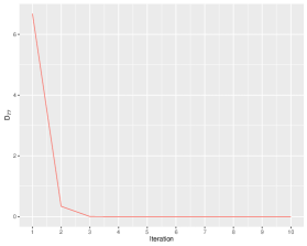
Figure 1: Plot of the iterates for $D_{77}$ for Sparse Cholesky in a setting with $p=8$. It shows how the value jumps to 0 (and stays there).

3.2 Simulated data: Graph Selection and Estimation

In this section, we perform a simulation study to compare the graph/model selection and estimation performance of CSCS, Sparse Cholesky and Sparse DAG. For model selection, we consider eight different settings with $p=1000,2000$ and $n=p/8,p/4,p/2,3p/2$. In particular, for each $p\in\{1000,2000\}$, a $p\times p$ lower triangular matrix $T_{0}$ is generated as follows. We randomly choose $98\%$ of the lower triangular entries, and set them to zero. The remaining $2\%$ entries are chosen randomly from a uniform distribution on $[0.3,0.7]$ and then assigned a positive/negative sign with probability $0.5$. Now, a $p\times p$ diagonal matrix $D_{0}$ is generated with diagonal entries chosen uniformly from $[2,5]$. For each sample size $n=p/8,p/4,p/2,3p/2$, $100$ datasets, each having i.i.d. multivariate normal distribution with mean zero and inverse covariance matrix $\Omega_{0}=T_{0}^{t}D_{0}^{-1}T_{0}$, are generated.

The model selection performance of the three algorithms, CSCS, Sparse Cholesky, Sparse DAG, is then compared using receiver operating characteristic (ROC) curves. These curves compare true positive rates (TPR) and false positive rates (FPR), and are obtained by varying the penalty parameter over roughly $40$ possible values. In applications, FPR is typically controlled to be sufficiently small, and therefore we restrict ourselves to settings where the FPR is less than 0.15. Area-under-the-curve is a standard measure used to compare model selection performance (see [3], [6]).

Tables 2 and 3 show the mean and standard deviation (over 100 simulations) for the area-under-the-curve for CSCS, Sparse Cholesky and Sparse DAG for $p=1000,2000$ and $n=p/8,p/4,p/2,3p/2$. It is clear that CSCS has a better model selection performance as compared to Sparse Cholesky and Sparse DAG for all the settings.

1. As expected Sparse Cholesky performs significantly worse that the other methods when $n<p$, but its comparative (and absolute) performance improves with increasing sample size, especially when $n>p$.

2. The tables also show that CSCS does better than Sparse DAG in terms of model selection, although the difference in AUC is not as drastic as with Sparse Cholesky. In should be noted that CSCS has a higher AUC than Sparse DAG for each of the $800$ datasets (100 each for $p=1000,2000$ and $n=p/8,p/4,p/2,3p/2$). We also note that the variability is much lower for CSCS than the other methods.

It is worth mentioning that for each of the $800$ datasets, the data was centered and scaled before running each method. This is done firstly to illustrate that scaling the data does not justify assuming that the latent variable conditional variances $\{D_{ii}\}_{i=1}^{p}$ are identically $1$, borne out by the consistently better model selection performance of CSCS as opposed to Sparse DAG. Secondly, we observed that the three algorithms typically run much faster when the data is scaled. Also, premultiplication of a multivariate normal vector by a diagonal matrix does not affect the sparsity pattern in the Cholesky factor of the inverse. Hence, given the extensive nature of our simulation study, we scaled the data in the interest of time.

As mentioned in Section 1, the assumption $\{D_{ii}\}_{i=1}^{p}$ are identically $1$ cannot be accounted for/justified by preprocessing the data, and can affect the estimation performance of the Sparse DAG approach. To illustrate this fact, we consider the settings $p=1000$ and $n=p/2,3p/2$ and generate $50$ datasets for a range of $\lambda$ values similar to the model selection experiment above. Figures 2 and 3 show the Frobenius norm difference (averaged over 50 independent repetitions) between the true inverse covariance matrix and the estimate ($||\Omega-\hat{\Omega}||_{F}$), where $\hat{\Omega}$ is the estimated inverse covariance matrix for CSCS and Sparse DAG for a range on penalty parameter values for $n=500$ and $n=1500$ respectively.

For each method (CSCS and Sparse DAG), we start with a penalty parameter value near zero ($0.01$) and increase it till the Frobenius norm error becomes constant, i.e., the penalty parameter is large enough so that all the off-diagonal entries of the Cholesky parameter are set to zero. That is why the range of penalty parameter values for the error curves is different in the (a) and (b) parts of Figures 2 and 3. For $n=500$, CSCS achieves a minimum error value of $19.9$ at $\lambda=0.2$, the maximum error value of $52.8$ is achieved at $\lambda=5$ (or higher) when the resulting estimate of $\Omega$ is a diagonal matrix with the $i^{th}$ diagonal entry given by $1/S_{ii}$ for $1\leq i\leq p$. On the the other hand, Sparse DAG achieves a minimum error value of $42$ at $\lambda=300$ (or higher) when the resulting estimate of $\Omega$ is the identity matrix, and achieves a maximum error value of $121.4$ at $\lambda=0.1$. If the penalty parameter is chosen by BIC (see Table 4) then CSCS has an error value of $22$ (corresponding to $\lambda=0.3$) and Sparse DAG has an error value of $97$ (corresponding to $\lambda=0.35$). A similar pattern is observed for the case $n=1500$. It is clear that CSCS has a significantly superior overall estimation performance than Sparse DAG in this setting.

	$\bf n=125$		$\bf n=250$		$\bf n=500$		$\bf n=1500$
Solver	Mean	Std. Dev.	Mean	Std. Dev.	Mean	Std. Dev.	Mean	Std. Dev.
Sparse Cholesky	0.012796	0.000045	0.018461	0.000108	0.078832	0.000122	0.127916	0.000027
Sparse DAG	0.113955	0.000200	0.129142	0.000048	0.135271	0.000066	0.138633	0.000026
CSCS	0.118440	0.000111	0.133958	0.000036	0.138492	0.000023	0.139891	0.000001

Table 2: Mean and Standard Deviation of area-under-the-curve (AUC) for 100 simulations for p = 1000. Each simulation yields a ROC curve from which the AUC is computed for FPR in the interval [0.01, 0.15]. CSCS achieves the highest AUC in each column.

	$\bf n=250$		$\bf n=500$		$\bf n=1000$		$\bf n=3000$
Solver	Mean	Std. Dev.	Mean	Std. Dev.	Mean	Std. Dev.	Mean	Std. Dev.
Sparse Cholesky	0.015131	0.000050	0.032391	0.000105	0.124284	0.000058	0.142678	0.000012
Sparse DAG	0.141957	0.000044	0.146362	0.000009	0.147984	0.000005	0.148742	0.000001
CSCS	0.144686	0.000019	0.147839	0.000004	0.148722	0.000002	0.148904	0.000001

Table 3: Mean and Standard Deviation of area-under-the-curve (AUC) for 100 simulations for p = 2000. Each simulation yields a ROC curve from which the AUC is computed for FPR in the interval [0.001, 0.15]. CSCS achieves the highest AUC in each column.

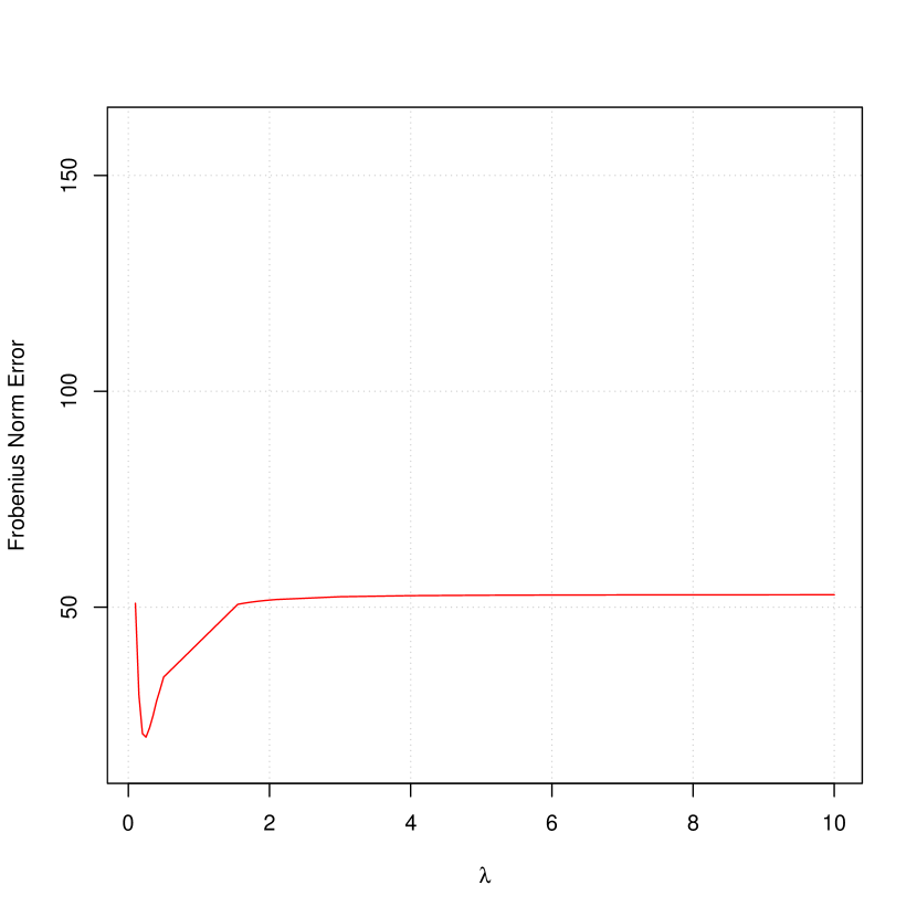
(a) Frobenius Norm Error for CSCS
(y-axis) with varying penalty parameter
value (x-axis) for $n=500$

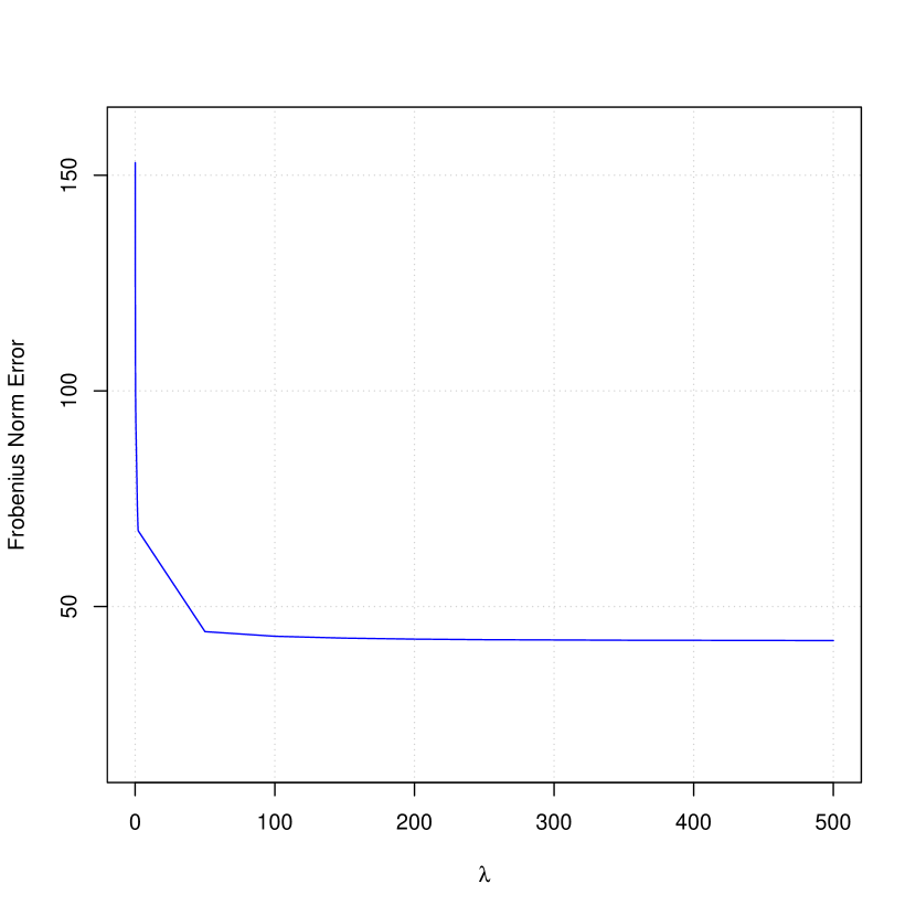
(b) Frobenius Norm Error for Sparse DAG averaged over 50 replications for $n=500$ for different penalty parameter values.

Figure 2:

	$n=500$	$n=1500$
CSCS	22.03 (0.09)	16.44 (0.06)
Sparse DAG	96.98(0.81)	108.90(0.14)

Table 4: Frobenius Norm error for $\lambda$ chosen by BIC for CSCS and Sparse DAG for $p=1000$

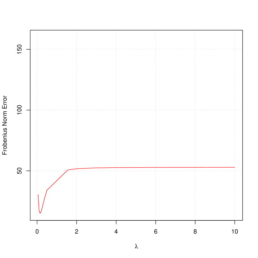
(a) Frobenius Norm Error for CSCS
(y-axis) with varying penalty parameter
value (x-axis) for $n=1500$

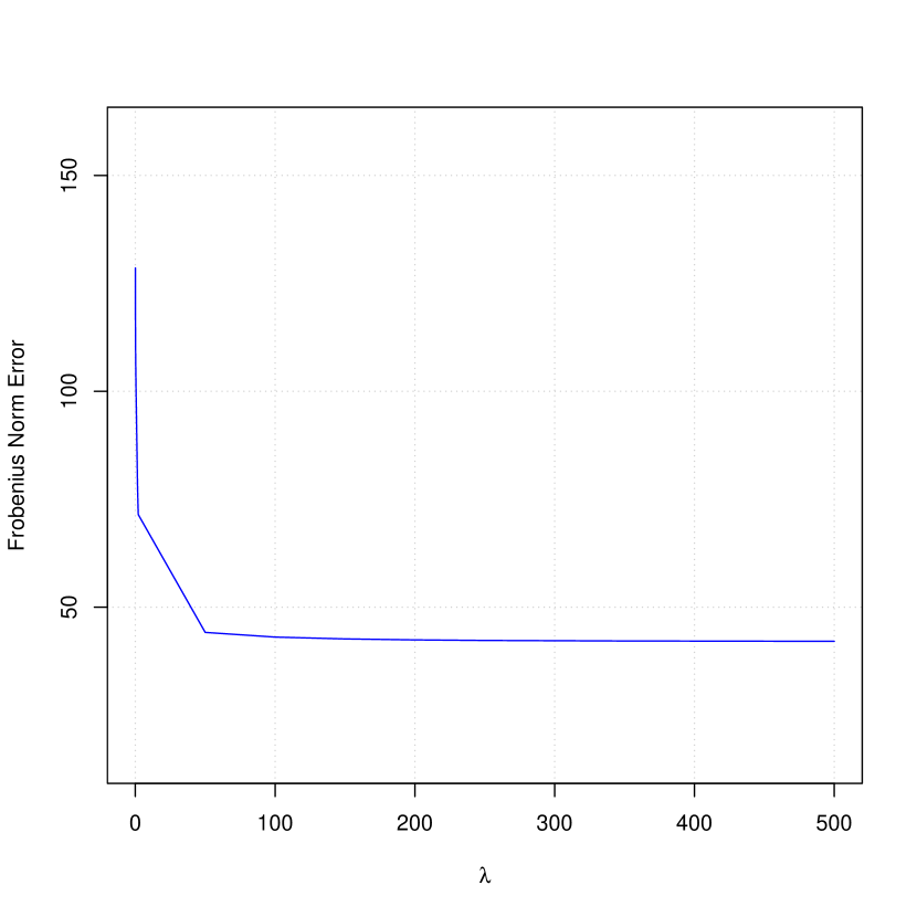
(b) Frobenius Norm Error for Sparse DAG averaged over 50 replications for $n=1500$ for different penalty parameter values.

Figure 3:

3.3 Application to genetics data

In this section, we analyze a flow cytometry dataset on p = 11 proteins and n = 7466 cells, from [21]. These authors fit a directed acyclic graph (DAG) to the data, producing the network in Figure 5(a). The ordering of the connections between pathway components were established based on perturbations in cells using molecular interventions and we consider the ordering to be known a priori.This dataset is analyzed in [5] and [23] using the Glasso algorithm and the Sparse DAG algotirms, respectively. In [5], the authors estimated the many graphs by varying the $\ell_{1}$ penalty and report around 50% false positive and false negative rates between one of the estimates and the findings of [21]. Figure 4 shows the true graph as well as the estimated graph using CSCS, Sparse Cholesky and Sparse DAG. We pick the penalty parameter by matching the sparsity to the true graph (approximately 72%). Here both Sparse DAG and CSCS perform better than Sparse Cholesky.

In [23], the authors recommend using the following equation for penalty parameter selection: $\lambda_{i}(\alpha)=2n^{-\frac{1}{2}}Z_{\frac{\alpha}{2p(i-1)}}^{*}$, where $Z_{q}^{*}*$ denotes the $(1-q)th$ quantile of the standard normal distribution. This choice uses a different penalty parameter for each row, and all the three penalized methods (Sparse Cholesky, Sparse DAG, CSCS) can be easily adapted to incorporate this. Using this method for Sparse DAG gives us a false positive rate of $0.46$ and a true positive rate of $0.78$, while Sparse Cholesky has a false positive rate of $0.62$ and a true positive rate of $0.94$. Hence, while Sparse Cholesky tends to find a lot of false edges, it fails to detect only one true edge. CSCS also fails to detect only one edge and thus has a true positive rate of $0.94$. However, it does better overall as indicated by the lower false positive rate at $0.51$. Figure 5 shows the true graph as well as the estimated graph using CSCS, Sparse Cholesky and Sparse DAG. By picking the penalty parameter according to BIC, Sparse Cholesky results in a completely sparse graph while CSCS and Sparse DAG return very dense graphs. The true and false positives for the 72% sparsity, normal quantile and BIC based estimates are provided in Table 5.

	72% Sparsity		$\lambda_{i}(\alpha)=2n^{-\frac{1}{2}}Z_{\frac{\alpha}{2p(i-1)}}^{*}$		BIC
Solver	FP	TP	FP	TP	FP	TP
CSCS	0.2432	0.5000	0.5135	0.9444	0.8649	1.0000
Sparse Cholesky	0.2703	0.4444	0.6216	0.9444	0.0000	0.0000
Sparse DAG	0.2432	0.5000	0.4595	0.7778	0.8108	1.0000

Table 5: TPR & FPR for Cell Signalling Pathway Data

(a) Sachs

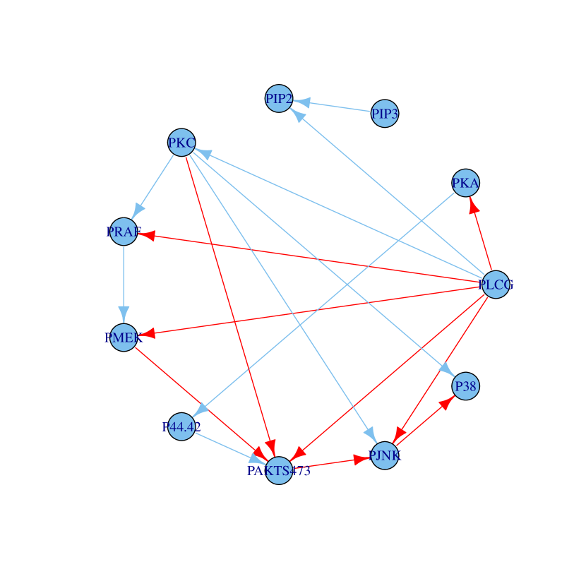
(b) CSCS

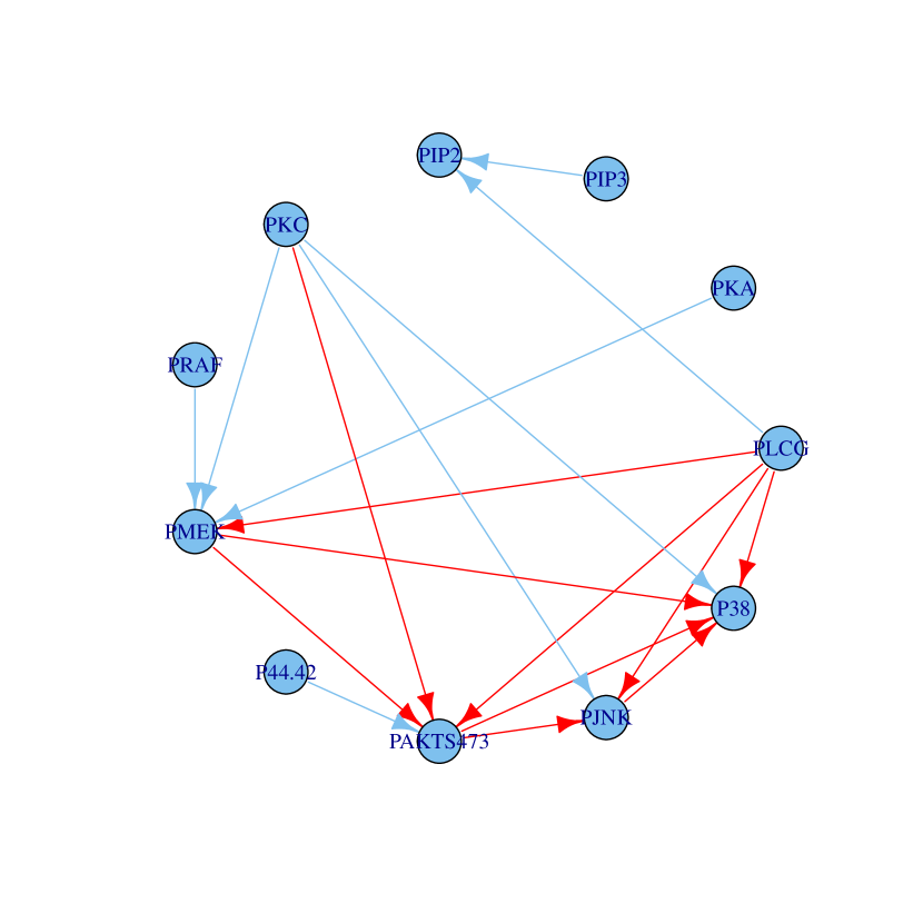
(c) Sparse Cholesky

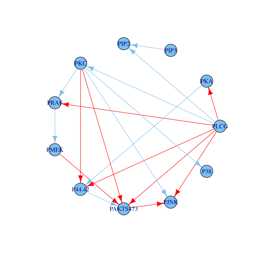
(d) Sparse DAG

Figure 4: True and estimated graphs from cell-signaling data. A blue arrow denotes a true positive, while a red arrow denotes a false positive

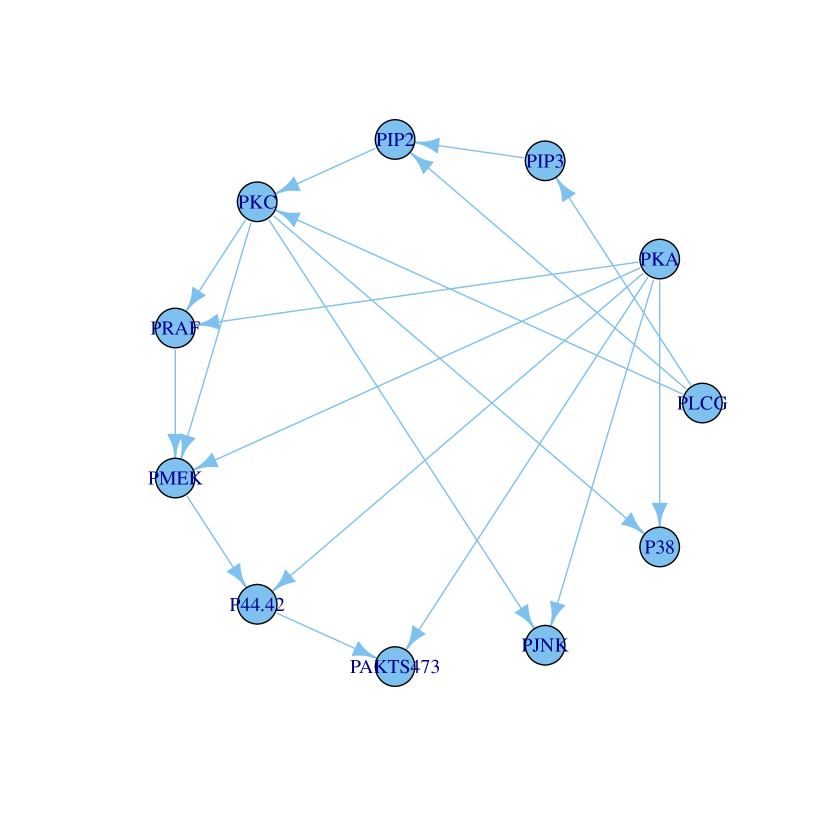
(a) Sachs

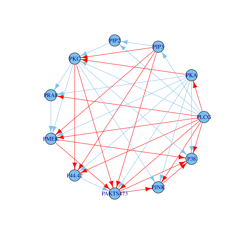
(b) CSCS

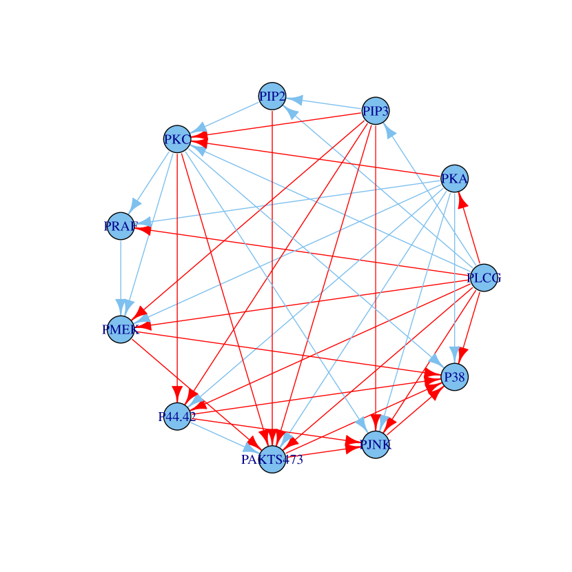
(c) Sparse Cholesky

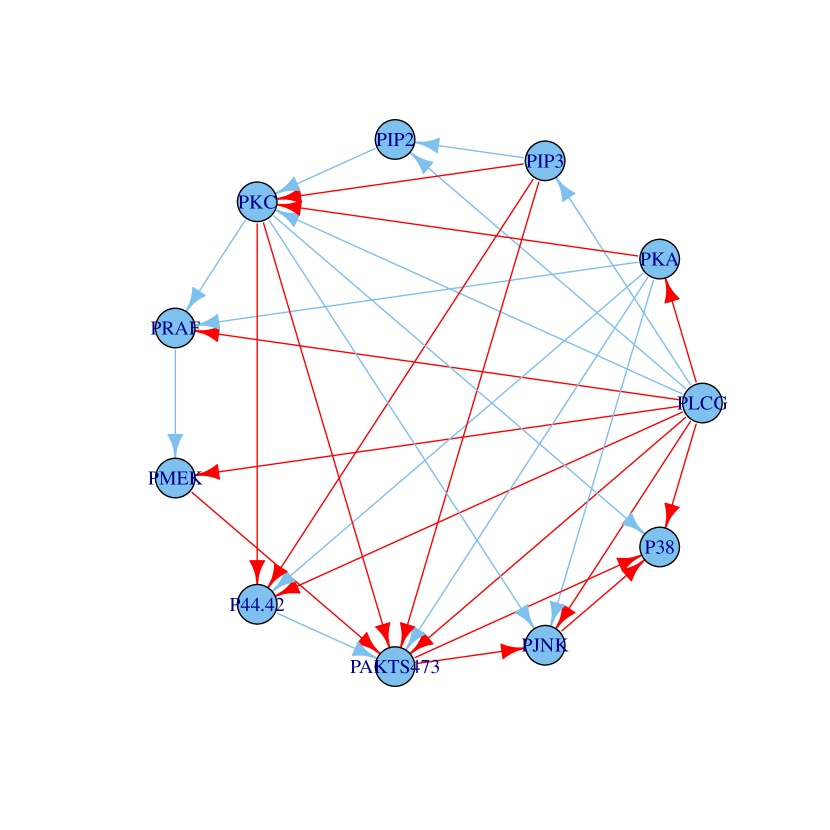
(d) Sparse DAG

Figure 5: True and estimated graphs from cell-signaling data by setting $\lambda_{i}(\alpha)=2n^{-\frac{1}{2}}Z_{\frac{\alpha}{2p(i-1)}}^{*}$. A blue arrow denotes a true positive, while a red arrow denotes a false positive

3.4 Application to call center data

In this section we discuss the application of CSCS, Sparse Cholesky and Sparse DAG to the call center data from [9]. The data, coming from one call center in a major U.S. northeastern financial organization, contain the information about the time every call arrives at the service queue. For each day in 2002, except for 6 days when the data-collecting equipment was out of order, phone calls are recorded from 7:00am until midnight. The 17-hour period is divided into 102 10-minute intervals, and the number of calls arriving at the service queue during each interval are counted. Since the arrival patterns of weekdays and weekends differ, the focus is on weekdays here. In addition, after using singular value decomposition to screen out outliers that include holidays and days when the recording equipment was faulty (see [22]), we are left with observations for 239 days.

The data were ordered by time period. Denote the data for day $i$ by $N_{i}=(N_{i,1},\ldots,N_{i,102})^{\prime}$, $i=1,\ldots,239$ where $N_{i,t}$ is the number of calls arriving at the call centre for the $t^{th}$ 10-minute interval on day $i$. Let $y_{it}=\sqrt{N_{it}+1/4},i=1,\ldots,239,t=1,\ldots,102$. We apply the three penalized likelihood methods (CSCS, Sparse DAG, Sparse Cholesky) to estimate the $102\times 102$ covariance matrix based on the residuals from a fit of the saturated mean model. Following the analysis in [9], the $\ell_{1}$ penalty parameter for all three methods was picked using $5$-fold cross validation on the training data set as follows. Randomly split the full dataset $D$ into $K$ subsets of about the same size, denoted by $D_{v},v=1,...,K$. For each $v$, we use the data $D-D_{v}$ to estimate $\Sigma_{-v}$ and $D_{v}$ to validate. Then pick $\lambda$ to minimize:

$$\text{CV}(\lambda)=\frac{1}{K}\sum_{v=1}^{K}\big{(}d_{v}\log|{\hat{\Sigma}_{-v}}|+\sum_{i\in I_{v}}y_{i}^{\prime}\hat{\Sigma}_{-v}^{-1}y_{i}\big{)}$$

where $I_{v}$ is the index set of the data in $D_{v}$, $d_{v}$ is the size of $I_{v}$, and $\hat{\Sigma}_{v}$ is the variance-covariance matrix estimated using the training data set $D-D_{v}$.

To assess the performance of different methods, we split the 239 days into training and test datasets. The data from the first $T$ days ($T=205,150,100,75$), form the training dataset that is used to estimate the mean vector and the covariance matrix. The mean vector is estimated by the mean of the training data vectors. Four different methods, namely, CSCS, Sparse Cholesky, Sparse DAG and S (sample covariance matrix) are used to get an estimate of the covariance matrix. For each of the three penalized methods, the penalty parameter is chosen both by cross-validation and the BIC criterion. Hence, we have a total of seven estimators for the covariance matrix. The log-likelihood for the test dataset (consisting of the remaining $239-T$ days) evaluated at all the above estimators is provided in Table 6. For all training data sizes, CSCS clearly demonstrates superior performance as compared to the other methods. Also, the comparative performance of CSCS with other methods improves significantly with decreasing training data size.

	Training Data Size
Method	$205$	$150$	$100$	$75$
CSCS-CV	-1090.447	-1369.181	-2225.907	-2841.348
CSCS-BIC	-1072.75	-1364.145	-2214.729	-2849.931
Sparse DAG-CV	-1077.791	-2237.298	-3576.343	-4499.298
Sparse DAG-BIC	-1135.980	-2421.950	-3817.689	-4846.118
Sparse Cholesky-CV	-1500.094	-2121.005	-3579.932	-496617558322
Sparse Cholesky-BIC	-1523.409	-2178.738	-3584.160	-5444.471
S	-1488.224	-7696.740	not pd	not pd

Table 6: Test data log-likelihood values for various estimation methods with training data size $205,150,100,75$. The maximum likelihood value in each column is written in bold.

Huang et al. [9] additionally use the estimated mean and covariance matrix to forecast the number of arrivals in the later half of the day using arrival patterns in the earlier half of the day. Following their method, we compared the performance of all the four methods under consideration (details provided in Supplemental Section F). We found that all the three penalized methods outperform the sample covariance matrix estimator. However, as far as this specific forecasting task is concerned, the differences in their performance compared to each other are marginal. We suspect that the for the purposes of this forecasting task, the estimated mean (same for all three methods) has a much stronger effect than the estimated covariance matrix. Hence the difference in forecasting performance is much smaller than the difference in likelihood values. Nevertheless, Sparse Cholesky has the best performance for training data size $T=205,150$ (when the sample size is more than the number of variables) and CSCS has the best performance for training data sizes $T=100,75$ (when the sample size is less than the number of variables). See Supplemental Section F for more details.

4 Asymptotic properties

In this section, asymptotic properties of the CSCS algorithm will be examined in a high-dimensional setting, where the dimension $p=p_{n}$ and the penalty parameter $\lambda=\lambda_{n}$ vary with $n$. In particular, we will establish estimation consistency and model selection consistency (oracle properties) for the CSCS algorithm under suitable regularity assumptions. Our approach is based on the strategy outlined in Meinshausen and Buhlmann [15] and Massam, Paul and Rajaratnam [13]. A similar approach was used by Peng et al. [18] to establish asymptotic properties of SPACE, which is a penalized pseudo likelihood based algorithm for sparse estimation of $\Omega$. Despite the similarity in the basic line of attack, there is an important structural difference between the asymptotic consistency arguments in [18] and this section (apart from the fact that we are imposing sparsity in $L$, not $\Omega$). For the purpose of proving asymptotic consistency, the authors in [18] assume that diagonal entries of $\Omega$ are known, thereby reducing their objective function to the sum of a quadratic term and an $\ell_{1}$ penalty term in $\Omega$. The authors in [23] also establish graph selection consistency of the Sparse DAG approach under the assumption that the diagonal entries of $L$ are $1$. We do not make such an assumption for $L$, which leaves us with $p$ additional non-zero parameters, and additional logarithmic terms in the objective function to work with. Nevertheless, we are able to adapt the basic consistency argument in this challenging setting with an almost identical set of regularity assumptions as in [18] (with assumptions on $\Omega$ replaced by the same assumptions on $L$). In particular, we only replace two assumptions in [18] with a weaker and a stronger version respectively (see Assumption (A4) and Assumption (A5) below for more details)

We start by establishing the required notation. Let $\{\bar{\Omega}_{n}=\bar{L}_{n}^{t}\bar{L}_{n}\}_{n\geq 1}$ denote the sequence of true inverse covariance matrices, and $\bar{\boldsymbol{\eta}}_{n}^{r}$ denote the lower triangular entries (including the diagonal) in the $r^{th}$ row of $\bar{L}_{n}$, for $1\leq r\leq p$. Let $\mathcal{A}_{n}^{r}$ denote the set of indices corresponding to non-zero entries in $r^{th}$ row of $\bar{L}_{n}$ for $1\leq r\leq p$, and let $q_{n}=\sum_{r=1}^{p_{n}}\left|\mathcal{A}_{n}^{r}\right|$. Let $\bar{\Sigma}_{n}=\bar{\Omega}_{n}^{-1}$ denote the true covariance matrix for every $n\geq 1$. The following standard assumptions are required.

• (A1 - Bounded eigenvalues) The eigenvalues of $\bar{\Omega}_{n}$ are bounded below by $\lambda_{min}>0$, and bounded above by $\lambda_{max}<\infty$ uniformly for all $n$.

• (A2 - Sub Gaussianity) The random vectors ${\bf Y}^{1},\dots,{\bf Y}^{n}$ are i.i.d. sub-Gaussian for every $n\geq 1$, i.e., there exists a constant $c>0$ such that for every ${\bf x}\in\mathbb{R}^{p_{n}}$, $E\left[e^{{\bf x}^{\prime}{\bf Y}^{i}}\right]\leq e^{c{\bf x}^{\prime}{\bf x}}$.

• (A3 - Incoherence condition) There exists $\delta<1$ such that for every $n\geq 1$, $1\leq r\leq p_{n}$ and $j\notin\mathcal{A}_{n}^{r}$,

  $$\left|\bar{\Sigma}_{n,j,\mathcal{A}^{r}}^{t}\left(\bar{\Sigma}_{n,\mathcal{A}^{r}\mathcal{A}^{r}}+\frac{2}{(\bar{\eta}_{r}^{r})^{2}}\Delta_{r}\right)^{-1}\mbox{sign}\left(\bar{\boldsymbol{\eta}}_{\mathcal{A}^{r}}^{r}\right)\right|\leq\delta.$$

  Here, $\Delta_{r}$ is a $|\mathcal{A}^{r}|\times|\mathcal{A}^{r}|$ matrix with

  $$(\Delta_{r})_{jj^{\prime}}=\begin{cases}1&\mbox{if }j=j^{\prime}=|\mathcal{A}^{r}|,\cr 0&\mbox{otherwise}.\end{cases}$$

• (A4 - Signal size) For every $n\geq 1$, let

  $$s_{n}=\min_{1\leq r\leq p}\min_{j\in\mathcal{A}_{n}^{r}}\left|\bar{\eta}^{r}_{n,j}\right|.$$

  Then $\frac{s_{n}}{\sqrt{d_{n}}\lambda_{n}}\rightarrow\infty$, where $d_{n}=\max_{1\leq r\leq p_{n}}|\mathcal{A}^{r}|$. This assumption will be useful for establishing sign consistency. The signal size condition in [18] is $\frac{s_{n}}{\sqrt{q_{n}}\lambda_{n}}\rightarrow\infty$, which is stronger than the signal size condition above, as $d_{n}\leq q_{n}$.

• (A5 - Growth of $p_{n}$, $q_{n}$ and $\lambda_{n}$) The following conditions hold: $p_{n}=O(n^{\kappa})$ for $\kappa\geq 0$, $q_{n}=o\left(\sqrt{\frac{n}{\log n}}\right)$, $\sqrt{\frac{q_{n}\log n}{n}}=o(\lambda_{n})$, $\lambda_{n}\sqrt{\frac{n}{\log n}}\rightarrow\infty$ and $q_{n}\lambda_{n}\rightarrow 0$ as $n\rightarrow\infty$. The growth conditions in [18] are the same as above (with $q_{n}$ denoting the sparsity in the true $\Omega$ in [18]), expect that $q_{n}\lambda_{n}\rightarrow 0$ above is replaced by the weaker assumption $\sqrt{q_{n}}\lambda_{n}\rightarrow 0$.

Under these assumptions, the following consistency result can be established.

Theorem 4.1

Suppose that (A1)-(A5) are satisfied. Then there exists a constant $C>0$, such that for any $\gamma>0$, the following events hold with probability at least $1-O(n^{-\eta})$:

1. A solution of the minimization problem

   $$\inf_{L\in\mathcal{L}_{p_{n}}}Q_{CSCS}(L)$$ (4.1)

   exists.

2. (Estimation and sign consistency): any solution $\hat{L}_{n}$ of the minimization problem in (4.1) satisfies

   $$\|\hat{L}_{n}-\bar{L}_{n}\|\leq Cq_{n}\lambda_{n}.$$

   and

   $$\mbox{sign}(\hat{L}_{n,ij})=\mbox{sign}(\bar{L}_{n,ij}),$$

   for every $1\leq j\leq i\leq p$.

Here $\mbox{sign}(x)$ takes the values $\{-1,0,1\}$ when $x<0$, $x=0$, and $x>0$ respectively. A proof of the above result is provided in the appendix.

5 Discussion

This paper proposes a novel penalized likelihood based approach for estimation and model selection in Gaussian DAG models. The goal is to overcome some of the shortcomings of current methods, but at the same time retain their respective strengths. We start with the objective function for the highly useful Sparse Cholesky approach in [9]. Reparametrization of this objective function in terms of the inverse of the classical Cholesky factor of the covariance matrix, along with appropriate changes to the penalty term, leads us to the formulation of the CSCS objective function. It is then shown that the CSCS objective function is jointly convex in its arguments. A coordinate-wise minimization algorithm that minimizes this objective, via closed form iterates, is proposed, and subsequently analyzed. The convergence of this coordinate-wise minimization algorithm to a global minimum is established rigorously. It is also established that the estimate produced by the CSCS algorithm always leads to a positive definite estimate of the covariance matrix - thus ensuring that CSCS leads to well defined estimates that are always computable. Such a guarantee is not available with the Sparse Cholesky approach when $n<p$. Large sample properties of CSCS establish estimation and model selection consistency of the method as both the sample size and dimension tend to infinity. We also point out that the Sparse DAG approach in [23], while always useful for graph selection, may suffer for estimation purposes due the assumption that the conditional variances $\{D_{ii}\}_{i=1}^{p}$ are identically $1$. The performance of CSCS compared to Sparse Cholesky and Sparse DAG is also illustrated via simulations and application to a cell-signaling pathway dataset and a call center dataset. These experiments complement and support the technical results in the paper by demonstrating the following.

1. When $n<p$, it is easy to find examples where Sparse Cholesky converges to its global minimum which corresponds to a singular covariance matrix (Section 3.1).

2. When $n<p$, the graph selection and estimation performance of CSCS is significantly better than Sparse Cholesky, due to the fact that Sparse Cholesky either converges to a global minimum with singularity issues, or to a local minimum (Section 3.2 and Section 3.4).

3. For graph selection, CSCS is competitive with Sparse DAG and can have better performance as compared to Sparse DAG. Although the improvement may not sometimes be as significant as that over Sparse Cholesky, these results demonstrate that CSCS is a useful addition to the high-dimensional DAG selection toolbox (Section 3.2 and Section 3.3).

4. For estimation purposes, CSCS can lead to significant improvements in performance over Sparse DAG (Section 3.2).

Supplemental Document for “A convex framework for high-dimensional sparse Cholesky based covariance estimation”

A Proof of Lemma 1.1

Note that $S_{n}$ (an $n\times n$ sample covariance matrix for the first $n$ variables) is non-singular with probaiblity $1$, while $S_{n+1}$ (an $(n+1)\times(n+1)$ matrix) is singular with probability $1$. Since

$$S_{n+1}=\left[\begin{matrix}S_{n}&S_{\cdot(n+1)}\cr S_{\cdot(n+1)}^{t}&S_{n+1,n+1}\end{matrix}\right],$$

is positive semi-definite, it follows that $S_{n+1,n+1}=S_{\cdot(n+1)}^{t}S_{n}^{-1}S_{\cdot(n+1)}$. Hence, if ${\boldsymbol{\phi}}_{n+1}^{*}=S_{n}^{-1}S_{\cdot(n+1)}$, we get that

$$({\boldsymbol{\phi}}_{n+1}^{*})^{t}S_{n}{\boldsymbol{\phi}}_{n+1}^{*}+2({\boldsymbol{\phi}}_{n+1}^{*})^{t}S_{\cdot(n+1)}+S_{n+1,n+1}=0.$$

It follows that

$$Q_{Chol,n+1}({\boldsymbol{\phi}}_{n+1}^{*},\frac{1}{m})=-\log m+\lambda\|{\boldsymbol{\phi}}_{n+1}^{*}\|_{1}\rightarrow-\infty$$

as $m\rightarrow\infty$. $\Box$

B Proof of Lemma 2.4

Note that for $1\leq j\leq k-1$,

$$h_{k,A,\lambda}({\bf x})=x_{j}^{2}A_{jj}+2x_{j}\left(\sum_{l\neq j}A_{lj}x_{l}\right)+\lambda|x_{j}|+\mbox{ terms independent of }x_{j}.$$

It follows that

$$\left(T_{j}({\bf x})\right)_{j}=\frac{S_{\lambda}\left(-2\sum_{l\neq j}A_{lj}x_{l}\right)}{2A_{jj}}.$$

Also,

$$h_{k,A,\lambda}({\bf x})=-2\log x_{k}+x_{k}^{2}A_{kk}+2x_{k}\left(\sum_{l\neq k}A_{lk}x_{l}\right)+\mbox{ terms independent of }x_{k}.$$

It follows that

$$\frac{\partial}{\partial x_{k}}h_{k,A,\lambda}({\bf x})=0 \Leftrightarrow -\frac{2}{x_{k}}+2x_{k}A_{kk}+2\sum_{l\neq k}A_{lk}x_{l}=0$$

$$\Leftrightarrow x_{k}=\frac{-\sum_{l\neq k}A_{lk}x_{l}+\sqrt{\left(\sum_{l\neq k}A_{lk}x_{l}\right)^{2}+4A_{kk}}}{2A_{kk}},$$

Note that since $x_{k}>0$ the positive root has been retained as the solution. $\Box$

C Proof of Lemma 2.6

We consider two cases.

Case 1 ($n\geq k$): It follows from (2.10) and (2.11) that the update for each of the $k$ coordinates in an iteration of Algorithm 1 can be achieved in $O(k)$ computations. Hence, a computational complexity of $O(k^{2})$ can be achieved in this case.

Case 2 ($n<k$): For this case, we will use ideas similar to the analysis of computational complexity in [1, 3, 4] in the context of algorithms inducing sparsity in $\Omega$. Let ${\bf r}({\bf x})=B^{T}{\bf x}\in\mathbb{R}^{n}$. Given the initial value $\hat{\bf x}^{(0)}$, we evaluate $r(\hat{\bf x}^{(0)})=B^{T}\hat{\bf x}^{(0)}$ (which takes $O(nk)$) iterations), and keep track of $B^{T}\hat{\bf x}^{\mbox{\scriptsize\,current}}$ throughout the course of the algorithm. Note that if ${\bf x}$ and $\tilde{\bf x}$ differ only in one coordinate (say the $m^{th}$ coordinate), then

$$(B^{T}\tilde{\bf x})_{j}=\sum_{l=1}^{k}B_{lj}\tilde{x}_{l}=\sum_{l=1}^{k}B_{lj}x_{l}+B_{mj}(\tilde{x}_{m}-x_{m})$$

for every $1\leq j\leq k$. It follows that it takes $O(n)$ computations to update $B^{T}{\bf x}$ to $B^{T}\tilde{\bf x}$. Hence, after each coordinatewise update in Algorithm 1, it will take $O(n)$ computations to update ${\bf r}$ to its current value. For every $1\leq j\leq k$, note that

$$\sum_{l\neq j}A_{lj}x_{l}=\sum_{l=1}^{k}A_{lj}x_{l}-A_{jj}x_{j}=B_{j\cdot}{\bf r}({\bf x})-A_{jj}x_{j}.$$

where $B_{j\cdot}$ denotes the $j^{th}$ row of the $k\times n$ matrix $B$. It now follows from (2.10) and (2.11) that each coordinatewise update in Algorithm 1 can be performed in $O(n)$ steps. Hence, the computational complexity of $O(nk)$ can be achieved for one iteration (which involves $k$ coordinatewise updates) of the Algorithm 1. $\Box$

D Proof of Theorem 2.1

Fix $1\leq i\leq p$ arbitrarily. Note that $S_{i}=\mathbb{Y}_{i}^{T}\mathbb{Y}_{i}$, where $\mathbb{Y}_{i}$ is an $n\times i$ matrix of observations corresponding to the first $i$ variables. Since all diagonal entries of $S$ are assumed to be positive, it follows that $\mathbb{Y}_{i}$ has no zero columns. Now, let $\xi\in\mathbb{R}$ be arbitrarily fixed. if $Q_{CSCS,i}({\boldsymbol{\eta}}^{i})<\xi$, then it follows that $-2\log\eta^{i}_{i}<\xi$ (since the other two terms in the expression for $Q_{CSCS,i}$ are non-negative). In particular, we obtain that $\eta^{i}_{i}>exp(-\xi/2)$. Also, it follows from (2.7) that $|\eta^{i}_{j}|\leq 2\xi/\lambda$ for every $1\leq j\leq i-1$, and $\eta^{i}_{i}\leq(\xi+b_{i})/a_{i}$. The above arguments, along with the expression for $Q_{CSCS,i}$ in (2.5) and (2.6), and [2, Theorem 2.2] imply that the cyclic coordinatewise algorithm for $Q_{CSCS,i}$ will converge to a global minimum of $Q_{CSCS,i}$. It follows that Algorithm 2 converges to a global minimum of $Q_{CSCS}$. $\Box$

E Proof of Theorem 4.1

Note that by (2.4), the problem of minimizing $Q_{CSCS}$ with respect to $L$ is equivalent to the problem of minimizing $Q_{CSCS,r}$ with respect to ${\boldsymbol{\eta}}^{r}$ for $1\leq r\leq p$. We will first establish appropriate consistency results for the minimizers of $Q_{CSCS,r}$, for each $1\leq r\leq p$, and then combine these results to establish Theorem 4.1. Throughout this proof, we will often suppress the dependence of various quantities on $n$, for notational simplicity and ease of exposition. We now establish a series of lemmas which will be quite useful in the main proof.

Lemma $\mathcal{S}$.1

For any $\gamma>0$, there exists a constant $C_{\gamma}>0$ such that with probability at least $1-O(n^{-\gamma})$

$$\max_{1\leq i,j,\leq p_{n}}|S_{ij}-\bar{\Sigma}_{n,ij}|\leq C_{\gamma}\sqrt{\frac{\log n}{n}}.$$

for large enough $n$.

Proof: Fix $1\leq i,j\leq p_{n}$. Let $\mu_{+}:=E_{\bar{\Sigma}_{n}}\left[(Y^{1}_{i}+Y^{1}_{j})^{2}\right]$ and $\mu_{-}:=E_{\bar{\Sigma}_{n}}\left[(Y^{1}_{i}-Y^{1}_{j})^{2}\right]$. It follows that

$$P(|S_{ij}-\bar{\Sigma}_{n,ij}|>t) \mathcal{S}$$ (.1)

$$= P\left(\left|\frac{1}{n}\sum_{\ell=1}^{n}(Y^{\ell}_{i}+Y^{\ell}_{j})^{2}-(Y^{\ell}_{i}-Y^{\ell}_{j})^{2}-(\mu_{+}-\mu_{-})\right|>4t\right)$$

$$\leq P\left(\left|\frac{1}{n}\sum_{\ell=1}^{n}(Y^{\ell}_{i}+Y^{\ell}_{j})^{2}-\mu_{+}\right|>2t\right)+P\left(\left|\frac{1}{n}\sum_{\ell=1}^{n}(Y^{\ell}_{i}-Y^{\ell}_{j})^{2}-\mu_{-}\right|>2t\right).$$

Note that $Y^{\ell}_{i}+Y^{\ell}_{j}$ are sub-Gaussian random variables (by Assumption (A2)) and their variances are uniformly bounded in $i$, $j$ and $n$ (by Assumption (A1)). For any $c_{1}>0$, it follows by ($\mathcal{S}$.1) and [5, Theorem 1.1], that there exist constants $K_{1}$ and $K_{2}$ independent of $i$, $j$ and $n$ such that

$$P\left(|S_{ij}-\bar{\Sigma}_{n,ij}|>C\sqrt{\frac{\log n}{n}}\right)\leq K_{1}e^{-K_{2}n\left(c_{1}\sqrt{\frac{\log n}{n}}\right)^{2}}=K_{1}e^{-K_{2}C^{2}\log n}$$

for large enough $n$. Using the union bound and the fact that $p=O(n^{\kappa})$ for some $\kappa\geq 0$ gives us the required result. $\Box$

Lemma $\mathcal{S}$.2

For every $1\leq r\leq p$, we note that ${\boldsymbol{\eta}}^{r}$ minimizes $Q_{CSCS,r}$ if and only if

$$d_{i}^{r}({\boldsymbol{\eta}}^{r})=-\lambda_{n}\mbox{sign}(\eta^{r}_{i})\mbox{ if }\eta^{r}_{i}\neq 0,\;1\leq i\leq r-1, \mathcal{S}$$ (.2)

$$|d_{i}^{r}({\boldsymbol{\eta}}^{r})|\leq\lambda_{n}\mbox{ if }\eta^{r}_{i}=0,1\leq i\leq r-1, \mathcal{S}$$ (.3)

$$d_{r}^{r}({\boldsymbol{\eta}}^{r})=0, \mathcal{S}$$ (.4)

where

$$d_{i}^{r}({\boldsymbol{\eta}}^{r})=2\sum_{j=1}^{r}\eta^{r}_{j}S_{ij} \mathcal{S}$$ (.5)

for $1\leq i\leq r-1$, and

$$d_{r}^{r}({\boldsymbol{\eta}}^{r})=2\sum_{j=1}^{r}\eta^{r}_{j}S_{rj}-\frac{2}{\eta^{r}_{r}}. \mathcal{S}$$ (.6)

Also, if $|d_{i}^{r}(\hat{\boldsymbol{\eta}}^{r})|<\lambda_{n}$ for any minimizer $\hat{\boldsymbol{\eta}}^{r}$, then by the continuity of $d_{i}^{r}$, and the convexity of $Q_{CSCS,r}$, it follows that $\tilde{\eta}_{i}^{r}=0$ for every minimizer $\tilde{\boldsymbol{\eta}}^{r}$ of $Q_{CSCS,r}$.

The proof immediately follows from the KKT conditions for the convex function $Q_{CSCS,r}$.

Lemma $\mathcal{S}$.3

For every $1\leq i\leq r\leq p$

$$E_{\bar{\Sigma}_{n}}\left[d_{i}^{r}(\bar{\boldsymbol{\eta}}_{n}^{r})\right]=0.$$

Proof: Let $\bar{\Sigma}_{n,r}$ denote the sub matrix of $\bar{\Sigma}_{n}$ formed by using the first $r$ rows and columns. Since $\bar{\Omega}_{n}=\bar{L}_{n}^{t}\bar{L}_{n}$, it follows that $\bar{\eta}^{r}_{n,r}\bar{\boldsymbol{\eta}}_{n}^{r}$ is the $r^{th}$ row of $\left(\bar{\Sigma}_{n,r}\right)^{-1}$. It follows that for every $1\leq i<r\leq p$,

$$E_{\bar{\Sigma}_{n}}\left[d_{i}^{r}(\bar{\eta}_{n}^{r})\right]=2\sum_{j=1}^{r}\bar{\eta}_{n,j}^{r}\bar{\Sigma}_{n,ij}=\frac{2}{\bar{\eta}^{r}_{r}}\sum_{j=1}^{r}\left(\bar{\Sigma}_{n,r}\right)^{-1}_{rj}\left(\bar{\Sigma}_{n,r}\right)_{ij}=0,$$

and

$$E_{\bar{\Sigma}_{n}}\left[d_{r}^{r}(\bar{\eta}_{n}^{r})\right]=\frac{2}{\bar{\eta}^{r}_{r}}\sum_{j=1}^{r}\left(\bar{\Sigma}_{n,r}\right)^{-1}_{rj}\left(\bar{\Sigma}_{n,r}\right)_{rj}-\frac{2}{\bar{\eta}_{r}^{r}}=0.$$

$\Box$

Lemma $\mathcal{S}$.4

For any $\gamma>0$, there exists a constant $C_{1,\gamma}>0$ such that with probability at least $1-O(n^{-\gamma})$,

$$\max_{1\leq i\leq r\leq p}|d_{i}^{r}(\bar{\boldsymbol{\eta}}_{n}^{r})|\leq C_{1,\eta}\sqrt{\frac{\log n}{n}}.$$

Proof: Note that

$$d_{i}^{r}(\bar{\boldsymbol{\eta}}_{n}^{r})=\frac{2}{n}\sum_{\ell=1}^{n}Y^{\ell}_{i}(\sum_{j=1}^{r}\bar{\eta}_{n,j}^{r}Y^{\ell}_{j})-\frac{2}{\bar{\eta}_{r}^{r}}1_{\{i=r\}}$$

is the difference between the sample covariance and population covariance of $Y_{i}$ and $\sum_{j=1}^{r}\bar{\eta}_{n,j}^{r}Y_{j}$ Since $\bar{\eta}^{r}_{n,r}\bar{\boldsymbol{\eta}}_{n}^{r}$ is the $r^{th}$ row of $\left(\bar{\Sigma}_{n,r}\right)^{-1}$, it follows by Assumption (A1) that the variance of $\sum_{j=1}^{r}\bar{\eta}_{n,j}^{r}Y_{j}$, given by $(\bar{\boldsymbol{\eta}}^{r})^{t}\Sigma_{n,r}\bar{\boldsymbol{\eta}}$ is uniformly bounded over $n$ and $r$. The proof now follows along the same lines as in the proof of Lemma $\mathcal{S}$.1. $\Box$

With the above lemmas in hand, we now move towards the main proof. Fix $r$ between $2$ and $p$ arbitrarily. Recall that $\mathcal{A}_{n}^{r}$ (henceforth referred to as $\mathcal{A}^{r}$) is the set of indices corresponding to the non-zero entries of $\bar{\boldsymbol{\eta}}_{n}^{r}$. We start by establishing properties for the following restricted minimization problem:

$$\mbox{Minimize }Q_{CSCS,r}({\boldsymbol{\eta}}^{r})\mbox{ w.r.t. }{\boldsymbol{\eta}}^{r}\mbox{ such that }\eta^{r}_{j}=0\mbox{ for every }j\notin\mathcal{A}^{r}. \mathcal{S}$$ (.7)

Lemma $\mathcal{S}$.5

There exists $C>0$ such that for any $\gamma>0$, a global minima of the restricted minimization problem in ($\mathcal{S}$.7) exists within the disc $\{{\boldsymbol{\eta}}^{r}:\|{\boldsymbol{\eta}}^{r}-\bar{\boldsymbol{\eta}}^{r}\|<C\sqrt{|\mathcal{A}^{r}|}\lambda_{n}\}$ with probability at least $1-O(n^{-\gamma})$ for sufficiently large $n$.

Proof: Let $\alpha_{n}=\sqrt{|\mathcal{A}^{r}|}\lambda_{n}$. Then for any constant $C>0$ and any ${\bf u}\in\mathbb{R}^{r}$ satisfying $u_{j}=0$ for every $j\notin\mathcal{A}^{r}$ and $\|{\bf u}\|=C$, we get by the triangle inequality that

$$\sum_{j=1}^{r-1}|\bar{\eta}^{r}_{j}|-\sum_{j=1}^{r-1}|\bar{\eta}^{r}_{j}+\alpha_{n}u_{j}|\leq\alpha_{n}\sum_{j=1}^{r-1}|u_{j}|\leq C\alpha_{n}\sqrt{|\mathcal{A}^{r}|}. \mathcal{S}$$ (.8)

Let

$$\tilde{Q}_{CSCS,r}({\boldsymbol{\eta}}^{r}):=({\boldsymbol{\eta}}^{r})^{T}S_{r}{\boldsymbol{\eta}}^{r}-2\log\eta^{r}_{r}.$$

By ($\mathcal{S}$.8) and a second order Taylor series expansion around $\bar{\boldsymbol{\eta}}^{r}$, we get

$$Q_{CSCS,r}(\bar{\boldsymbol{\eta}}^{r}+\alpha_{n}{\bf u})-Q_{CSCS,r}(\bar{\boldsymbol{\eta}}^{r}) \mathcal{S}$$ (.9)

$$= \tilde{Q}_{CSCS,r}(\bar{\boldsymbol{\eta}}^{r}+\alpha_{n}{\bf u})-\tilde{Q}_{CSCS,r}(\bar{\boldsymbol{\eta}}^{r})-\lambda_{n}\left(\sum_{j=1}^{r-1}|\bar{\eta}^{r}_{j}|-\sum_{j=1}^{r-1}|\bar{\eta}^{r}_{j}+\alpha_{n}u_{j}|\right)$$

$$\geq \alpha_{n}\sum_{j\in\mathcal{A}^{r}}u_{j}d_{j}^{r}(\bar{\boldsymbol{\eta}}^{r})+\alpha_{n}^{2}\sum_{j\in\mathcal{A}^{r}}\sum_{k\in\mathcal{A}^{r}}u_{j}u_{k}S_{jk}+\frac{u_{r}^{2}}{2(\eta^{r}_{*})^{2}}-C\alpha_{n}\sqrt{|\mathcal{A}^{r}|}\lambda_{n}$$

$$\geq \alpha_{n}\sum_{j\in\mathcal{A}^{r}}u_{j}d_{j}^{r}(\bar{\boldsymbol{\eta}}^{r})+\alpha_{n}^{2}\sum_{j\in\mathcal{A}^{r}}\sum_{k\in\mathcal{A}^{r}}u_{j}u_{k}(S_{jk}-\bar{\Sigma}_{n,jk})+\sum_{j\in\mathcal{A}^{r}}\sum_{k\in\mathcal{A}^{r}}u_{j}u_{k}\bar{\Sigma}_{n,jk}-C\alpha_{n}^{2}$$

where $\eta^{r}_{*}\in[\bar{\eta}_{r}^{r},\bar{\eta}_{r}^{r}+\alpha_{n}u_{r}]$. Note that $\lambda_{n}\sqrt{\frac{n}{\log n}}\rightarrow\infty$, and $q_{n}\sqrt{\frac{\log n}{n}}\rightarrow 0$ as $n\rightarrow\infty$, by Assumption (A1). It follows by Cauchy-Schwarz inequality, Lemma $\mathcal{S}$.1 and Lemma $\mathcal{S}$.4 that for any $\gamma>0$, there exist constants $C_{\gamma}$ and $C_{1,\gamma}>0$ such that with probability at least $1-O(n^{-\gamma})$,

$$\alpha_{n}\sum_{j\in\mathcal{A}^{r}}u_{j}d_{j}^{r}(\bar{\boldsymbol{\eta}}^{r})\leq CC_{1,\gamma}\sqrt{\frac{|\mathcal{A}^{r}|\log n}{n}}\alpha_{n}=o(\alpha_{n}^{2}), \mathcal{S}$$ (.10)

and

$$\frac{\alpha_{n}^{2}}{2}|\sum_{j\in\mathcal{A}^{r}}\sum_{k\in\mathcal{A}^{r}}u_{j}u_{k}(S_{jk}-\bar{\Sigma}_{n,jk})|\leq C_{\gamma}C^{2}q_{n}\sqrt{\frac{\log n}{n}}=o(\alpha_{n}^{2}). \mathcal{S}$$ (.11)

Also, by Assumption A1, it follows that

$$\sum_{j\in\mathcal{A}^{r}}\sum_{k\in\mathcal{A}^{r}}u_{j}u_{k}\bar{\Sigma}_{n,jk}\geq\frac{C^{2}\alpha_{n}^{2}}{2\lambda_{max}}. \mathcal{S}$$ (.12)

Combining ($\mathcal{S}$.9), ($\mathcal{S}$.10), ($\mathcal{S}$.11) and ($\mathcal{S}$.12), we get that

$$Q_{CSCS,r}(\bar{\boldsymbol{\eta}}^{r}+\alpha_{n}{\bf u})-Q_{CSCS,r}(\bar{\boldsymbol{\eta}}^{r})>\frac{C^{2}\alpha_{n}^{2}}{2\lambda_{max}}-2C\alpha_{n}^{2}$$

with probability at least $1-O(n^{-\gamma})$ for large enough $n$. Choosing $C=4\lambda_{max}+1$, we obtain that

$$\inf_{{\bf u}:{\bf u}_{j}=0forj\notin\mathcal{A}^{r},\|{\bf u}\|=C}Q_{CSCS,r}(\bar{\boldsymbol{\eta}}^{r}+\alpha_{n}{\bf u})>Q_{CSCS,r}(\bar{\boldsymbol{\eta}}^{r}),$$

with probability at least $1-O(n^{-\gamma})$ for large enough$n$. Hence for every $\eta>0$, a local minima (in fact global minima due to convexity) of the restricted minimization problem in ($\mathcal{S}$.7) exists within the disc $\{{\boldsymbol{\eta}}^{r}:\|{\boldsymbol{\eta}}^{r}-\bar{\boldsymbol{\eta}}^{r}\|<C\sqrt{|\mathcal{A}^{r}|}\lambda_{n}\}$ with probability at least $1-O(n^{-\eta})$ for sufficiently large $n$. $\Box$

Lemma $\mathcal{S}$.6

There exists a constant $C_{1}>0$, such that for any $\gamma>0$ the following holds with probability $1-O(n^{-\gamma})$: for any ${\boldsymbol{\eta}}^{r}$ in the set

$$S=\{{\boldsymbol{\eta}}^{r}:\|{\boldsymbol{\eta}}^{r}-\bar{\boldsymbol{\eta}}^{r}\|\geq C_{1}\sqrt{|\mathcal{A}^{r}|}\lambda_{n},\;\eta_{j}^{r}=0\;\forall j\notin\mathcal{A}^{r}\},$$

we have $\left\|{\bf d}_{\mathcal{A}^{r}}^{r}(\bar{\boldsymbol{\eta}}^{r})\right\|>\sqrt{|\mathcal{A}^{r}|}\lambda_{n}$, where ${\bf d}_{\mathcal{A}^{r}}^{r}(\bar{\boldsymbol{\eta}}^{r}):=\left(d_{j}^{r}(\bar{\boldsymbol{\eta}}^{r})\right)_{j\in\mathcal{A}^{r}}$.

Proof: Recall that $\alpha_{n}=\sqrt{|\mathcal{A}^{r}|}\lambda_{n}$. Choose ${\boldsymbol{\eta}}\in S$ arbitrarily. Let ${\bf u}={\boldsymbol{\eta}}^{r}-\bar{\boldsymbol{\eta}}^{r}/\alpha_{n}$. It follows that $u_{j}=0$ for every $j\notin\mathcal{A}^{r}$, and $\|{\bf u}\|\geq C_{1}$. Let $\Delta_{r}$ denote the $|\mathcal{A}^{r}|\times|\mathcal{A}^{r}|$ matrix with the diagonal entry corresponding to the $r^{th}$ variable equal to $1$, and all other entries equal to zero. By a first order Taylor series expansion ${\bf d}_{\mathcal{A}^{r}}^{r}$, it follows that

$${\bf d}_{\mathcal{A}^{r}}^{r}({\boldsymbol{\eta}}^{r}) = {\bf d}_{\mathcal{A}^{r}}^{r}(\bar{\boldsymbol{\eta}}^{r})+2\alpha_{n}\left(S_{\mathcal{A}^{r}\mathcal{A}^{r}}+\frac{1}{({\boldsymbol{\eta}}^{r}_{*})^{2}}\Delta_{r}\right){\bf u}_{\mathcal{A}^{r}}$$

$$= {\bf d}_{\mathcal{A}^{r}}^{r}(\bar{\boldsymbol{\eta}}^{r})+2\alpha_{n}\left(\Sigma_{\mathcal{A}^{r}\mathcal{A}^{r}}+\frac{1}{(\eta_{*}^{r})^{2}}\Delta_{r}\right){\bf u}_{\mathcal{A}^{r}}+2\alpha_{n}\left(S_{\mathcal{A}^{r}\mathcal{A}^{r}}-\Sigma_{n,\mathcal{A}^{r}\mathcal{A}^{r}}\right){\bf u}_{\mathcal{A}^{r}},$$

where $\eta_{r}^{*}$ lies between $\bar{\eta}_{r}^{r}$ and $\bar{\eta}_{r}^{r}+\alpha_{n}u_{r}$. By Lemma $\mathcal{S}$.1 and Lemma $\mathcal{S}$.4 it follows that for any $\gamma>0$, there exist constants $C_{2,\gamma}$ and $C_{3,\gamma}$ such that

$$\|{\bf d}_{\mathcal{A}^{r}}^{r}({\boldsymbol{\eta}}^{r})\|$$

$$\geq 2\alpha_{n}\left\|\left(\Sigma_{\mathcal{A}^{r}\mathcal{A}^{r}}+\frac{1}{({\boldsymbol{\eta}}^{r}_{*})^{2}}\Delta_{r}\right){\bf u}_{\mathcal{A}^{r}}\right\|-C_{2,\gamma}\sqrt{\frac{q_{n}\log n}{n}}-C_{3,\gamma}\|{\bf u}\|\frac{\alpha_{n}|\mathcal{A}^{r}|\sqrt{\log n}}{\sqrt{n}}$$

$$\geq \frac{\alpha_{n}}{\lambda_{max}}\|{\bf u}\|=\sqrt{|\mathcal{A}^{r}|}\lambda_{n}\frac{C_{1}}{\lambda_{max}}$$

with probability at least $1-O(n^{-\gamma})$, for large enough $n$. The last inequality follows from Assumption (A1), the fact that $|\mathcal{A}^{r}|\leq q_{n}$ and Assumption (A5). Choosing $C_{1}=\lambda_{max}+1$ leads to the required result. $\Box$

The next lemma establishes estimation and model selection (sign) consistency for the restricted minimization problem in ($\mathcal{S}$.7).

Lemma $\mathcal{S}$.7

There exists $C_{2}>0$ such that for any $\gamma>0$, the following holds with probability $1-O(n^{-\gamma})$, for large enough $n$: (i) there exists a solution to the minimization problem in ($\mathcal{S}$.7), (ii) (estimation consistency) any global minimum of the restricted minimization problem in ($\mathcal{S}$.7) lies within the disc $\{{\boldsymbol{\eta}}^{r}:\|{\boldsymbol{\eta}}^{r}-\bar{\boldsymbol{\eta}}^{r}\|<C_{2}\sqrt{|\mathcal{A}^{r}|}\lambda_{n}\}$, and (iii) (sign consistency) for any solution $\hat{\boldsymbol{\eta}}^{r}$ of the minimization problem in ($\mathcal{S}$.7), $\mbox{sign}(\hat{\eta}_{j})=\mbox{sign}(\bar{\eta}_{j})$ for every $1\leq j\leq r$.

Proof: The existence of a solution follows from Lemma $\mathcal{S}$.6. By the KKT conditions for the restricted minimization problem in ($\mathcal{S}$.7) (along the lines of Lemma $\mathcal{S}$.2), it follows that for any solution $\hat{\boldsymbol{\eta}}^{r}$ of ($\mathcal{S}$.7), $|d_{j}^{r}(\hat{\boldsymbol{\eta}}^{r})|\leq\lambda_{n}$ for every $j\in\mathcal{A}^{r}$. It follows that $\left\|{\bf d}_{\mathcal{A}^{r}}^{r}(\hat{\boldsymbol{\eta}}^{r})\right\|\leq\sqrt{\mathcal{A}^{r}}\lambda_{n}$. The estimation consistency now follows from Lemma $\mathcal{S}$.7. Note that by Assumption (A4), $\bar{\eta}_{j}^{r}\geq s_{n}>2C_{2}\sqrt{|\mathcal{A}^{r}|}\lambda_{n}$ for every $j\in\mathcal{A}^{r}$, for sufficiently large $n$. The sign consistency now follows by combining this fact with $\|{\boldsymbol{\eta}}^{r}-\bar{\boldsymbol{\eta}}^{r}\|<C_{2}\sqrt{|\mathcal{A}^{r}|}\lambda_{n}$. $\Box$

The next lemma will be instrumental in showing that the solution set of the restricted minimization problem in ($\mathcal{S}$.7) is the same as the solution set of the unrestricted minimization problem for $Q_{CSCS,r}$ with high probability.

Lemma $\mathcal{S}$.8

For any $\gamma>0$, any solution $\hat{\boldsymbol{\eta}}^{r}$ of ($\mathcal{S}$.7) satisfies

$$\max_{j\notin\mathcal{A}^{r}}\left|d_{j}^{r}(\hat{\boldsymbol{\eta}}^{r})\right|<\lambda_{n}$$

with probability at least $1-O(n^{-\gamma})$, for large enough $n$.

Proof: Let $\gamma>0$ be given, and let $\hat{\boldsymbol{\eta}}^{r}$ be a solution of ($\mathcal{S}$.7). If $C_{n}:=\{\mbox{sign}(\hat{\boldsymbol{\eta}}^{r})=\mbox{sign}(\bar{\boldsymbol{\eta}}^{r})\}$, then $P(C_{n})\geq 1-O(n^{-\gamma-\kappa})$ for large enough $n$ (by Lemma $\mathcal{S}$.7). Now, on $C_{n}$, it follows by the a first order expansion of ${\bf d}_{\mathcal{A}^{r}}^{r}$ around $\bar{\boldsymbol{\eta}}^{r}$, and the KKT conditions for ($\mathcal{S}$.7) that

$$-\lambda_{n}\mbox{sign}\left(\bar{\boldsymbol{\eta}}_{\mathcal{A}^{r}}^{r}\right) = {\bf d}_{\mathcal{A}^{r}}^{r}(\hat{\boldsymbol{\eta}}^{r}) \mathcal{S}$$ (.14)

$$= {\bf d}_{\mathcal{A}^{r}}^{r}(\bar{\boldsymbol{\eta}}^{r})+2S_{\mathcal{A}^{r}\mathcal{A}^{r}}\hat{\bf u}_{n}+\frac{2}{(\eta_{r}^{*})^{2}}\Delta_{r}\hat{\bf u}_{n}$$

$$= H_{n}\hat{\bf u}_{n}+{\bf d}_{\mathcal{A}^{r}}^{r}(\bar{\boldsymbol{\eta}}^{r})+2\left(S_{\mathcal{A}^{r}\mathcal{A}^{r}}-\bar{\Sigma}_{n,\mathcal{A}^{r}\mathcal{A}^{r}}\right)\hat{\bf u}_{n}+$$

$$\left(\frac{2}{(\eta_{r}^{*})^{2}}-\frac{2}{(\bar{\eta}_{r}^{r})^{2}}\right)\Delta_{r}\hat{\bf u}_{n},$$

where $\hat{\bf u}_{n}=\hat{\boldsymbol{\eta}}^{r}-\bar{\boldsymbol{\eta}}^{r}$, $\eta_{r}^{*}$ lies between $\bar{\eta}_{r}^{r}$ and $\hat{\eta}_{r}^{r}$, and $H_{n}=2\bar{\Sigma}_{n,\mathcal{A}^{r}\mathcal{A}^{r}}+\frac{2}{(\bar{\eta}_{r}^{r})^{2}}\Delta_{r}$. Hence,

$$\hat{\bf u}_{n} = -\lambda_{n}H_{n}^{-1}\mbox{sign}\left(\bar{\boldsymbol{\eta}}_{\mathcal{A}^{r}}^{r}\right)-H_{n}^{-1}{\bf d}_{\mathcal{A}^{r}}^{r}(\bar{\boldsymbol{\eta}}^{r})-2H_{n}^{-1}\left(S_{\mathcal{A}^{r}\mathcal{A}^{r}}-\bar{\Sigma}_{n,\mathcal{A}^{r}\mathcal{A}^{r}}\right)\hat{\bf u}_{n} \mathcal{S}$$ (.15)

$$-2H_{n}^{-1}\left(\frac{1}{(\eta_{r}^{*})^{2}}-\frac{1}{(\bar{\eta}_{r}^{r})^{2}}\right)\Delta_{r}\hat{\bf u}_{n}.$$

Now, let us fix $j\notin\mathcal{A}^{r}$. By a first order Taylor series expansion of $d_{j}^{r}$, it follows that

$$d_{j}^{r}(\hat{\boldsymbol{\eta}}^{r})=d_{j}^{r}(\bar{\boldsymbol{\eta}}^{r})+2S_{i,\mathcal{A}^{r}}^{t}\hat{\bf u}_{n}.$$

Using ($\mathcal{S}$.15), we get that

$$d_{j}^{r}(\hat{\boldsymbol{\eta}}^{r}) = d_{j}^{r}(\bar{\boldsymbol{\eta}}^{r})+2(S_{j,\mathcal{A}^{r}}-\bar{\Sigma}_{n,j,\mathcal{A}^{r}})^{t}\hat{\bf u}_{n}+2\bar{\Sigma}_{n,j,\mathcal{A}^{r}}^{t}\hat{\bf u}_{n} \mathcal{S}$$ (.16)

$$= -2\lambda_{n}\bar{\Sigma}_{n,j,\mathcal{A}^{r}}^{t}H_{n}^{-1}\mbox{sign}\left(\bar{\boldsymbol{\eta}}_{\mathcal{A}^{r}}^{r}\right)+d_{j}^{r}(\bar{\boldsymbol{\eta}}^{r})-2\bar{\Sigma}_{n,j,\mathcal{A}^{r}}^{t}H_{n}^{-1}{\bf d}_{\mathcal{A}^{r}}^{r}(\bar{\boldsymbol{\eta}}^{r})+$$

$$-4\bar{\Sigma}_{n,j,\mathcal{A}^{r}}^{t}H_{n}^{-1}\left(S_{\mathcal{A}^{r}\mathcal{A}^{r}}-\bar{\Sigma}_{n,\mathcal{A}^{r}\mathcal{A}^{r}}\right)\hat{\bf u}_{n}-4\Sigma_{n,j,\mathcal{A}^{r}}^{t}H_{n}^{-1}\left(\frac{1}{(\eta_{r}^{*})^{2}}-\frac{1}{(\bar{\eta}_{r}^{r})^{2}}\right)\Delta_{r}\hat{\bf u}_{n}+$$

$$2(S_{i,\mathcal{A}^{r}}-\bar{\Sigma}_{n,i,\mathcal{A}^{r}})^{t}\hat{\bf u}_{n}.$$

We now individually analyze all the terms in ($\mathcal{S}$.16). It follows by the “incoherence” Assumption (A3) that the first term satisfies

$$\left|-2\lambda_{n}\bar{\Sigma}_{n,j,\mathcal{A}^{r}}^{t}H_{n}^{-1}\mbox{sign}\left(\bar{\boldsymbol{\eta}}_{\mathcal{A}^{r}}^{r}\right)\right|\leq\delta\lambda_{n}<\lambda_{n}. \mathcal{S}$$ (.17)

It follows by Lemma $\mathcal{S}$.4 and Assumption (A5) that the second term $d_{j}^{r}(\bar{\boldsymbol{\eta}}^{r})$ is $o(\lambda_{n})$ with probability $1-O(n^{-\gamma-\kappa})$ for large enough $n$. Also, by Assumption (A1) and the definition of $H_{n}$, we get that

$$\left\|2\bar{\Sigma}_{n,j,\mathcal{A}^{r}}^{t}H_{n}^{-1}\right\|\leq\left\|\bar{\Sigma}_{n,j,\mathcal{A}^{r}}\right\|\|2H_{n}^{-1}\|\leq\frac{1}{\lambda_{min}}\left\|\Sigma_{n,\mathcal{A}^{r}\mathcal{A}^{r}}^{-1}\right\|\leq\frac{\lambda_{max}}{\lambda_{min}}. \mathcal{S}$$ (.18)

It follows by Lemma $\mathcal{S}$.4 and Assumption (A5) that the third term in ($\mathcal{S}$.16) satisfies

$$\left|2\bar{\Sigma}_{n,j,\mathcal{A}^{r}}^{t}H_{n}^{-1}{\bf d}_{\mathcal{A}^{r}}^{r}(\bar{\boldsymbol{\eta}}^{r})\right|\leq\frac{\lambda_{max}}{\lambda_{min}}\sqrt{q_{n}}\max_{j\in\mathcal{A}^{r}}|d_{j}^{r}(\bar{\boldsymbol{\eta}}^{r})|=o(\lambda_{n}). \mathcal{S}$$ (.19)

Let ${\bf b}=2H_{n}^{-1}\Sigma_{n,j,\mathcal{A}^{r}}$. Note that by ($\mathcal{S}$.18), the norm of $\{\bf b\}$ is uniformly bounded in $n$ and $r$. Note that the $j^{th}$ element of the vector $\left(S_{\mathcal{A}^{r}\mathcal{A}^{r}}-\bar{\Sigma}_{n,\mathcal{A}^{r}\mathcal{A}^{r}}\right){\bf b}$ is the difference between the sample and the population covariance of $Y_{j}$ and $\sum_{k\in\mathcal{A}^{r}}b_{k}Y_{k}$. Using the same line of arguments as in the proof of Lemma $\mathcal{S}$.4, it follows that there exists a constant $C_{4,\gamma}>0$ such that

$$\max_{j\in\mathcal{A}^{r}}\left|\left(\left(S_{\mathcal{A}^{r}\mathcal{A}^{r}}-\bar{\Sigma}_{n,\mathcal{A}^{r}\mathcal{A}^{r}}\right){\bf b}\right)_{j}\right|\leq C_{4,\gamma}\sqrt{\frac{\log n}{n}}, \mathcal{S}$$ (.20)

with probability $1-O(n^{-\gamma-\kappa})$, for large enough $n$. By ($\mathcal{S}$.18), ($\mathcal{S}$.20), the estimation consistency part of Lemma $\mathcal{S}$.7 and Assumption (A5) that the fourth term in ($\mathcal{S}$.16) satisfies

$$\left|4\bar{\Sigma}_{n,j,\mathcal{A}^{r}}^{t}H_{n}^{-1}\left(S_{\mathcal{A}^{r}\mathcal{A}^{r}}-\bar{\Sigma}_{n,\mathcal{A}^{r}\mathcal{A}^{r}}\right)\hat{\bf u}_{n}\right| \leq 2\left\|\left(S_{\mathcal{A}^{r}\mathcal{A}^{r}}-\bar{\Sigma}_{n,\mathcal{A}^{r}\mathcal{A}^{r}}\right){\bf b}\right\|\|\hat{\bf u}_{n}\| \mathcal{S}$$ (.21)

$$= O\left(\sqrt{\frac{|\mathcal{A}^{r}\log n}{n}}\sqrt{|\mathcal{A}^{r}|}\lambda_{n}\right)=o(\lambda_{n}),$$

with probability $1-O(n^{-\gamma-\kappa})$, for large enough $n$. Since $(\bar{\eta}_{r}^{r})^{2}$ is the $r^{th}$ diagonal entry of $\bar{\Sigma}_{n,r}^{-1}$, it follows by Assumption (A1) that $\bar{\eta}_{r}^{r}$ is uniformly bounded above and below in $n$ and $r$. Since $\eta_{r}^{*}$ lies between $\bar{\eta}_{r}^{r}$ and $\hat{\eta}_{r}^{r}$, it follows by the estimation consistency part of Lemma $\mathcal{S}$.7 that $\eta_{r}^{*}$ is bounded above and below uniformly with probability at least $1-O(n^{-\gamma-\kappa})$, for large enough $n$. By ($\mathcal{S}$.18), the definition of $\Delta_{r}$, Lemma $\mathcal{S}$.7, and Assumption (A1), the fifth term in ($\mathcal{S}$.16) satisfies

$$\left|4\Sigma_{n,j,\mathcal{A}^{r}}^{t}H_{n}^{-1}\left(\frac{1}{(\eta_{r}^{*})^{2}}-\frac{1}{(\bar{\eta}_{r}^{r})^{2}}\right)\Delta_{r}\hat{\bf u}_{n}\right| \leq \frac{2\lambda_{max}|\bar{\eta}_{r}^{r}+\eta_{r}^{*}||}{\lambda_{min}(\bar{\eta}_{r}^{r})^{2}(\eta_{r}^{*})^{2}}|\bar{\eta}_{r}^{r}-\hat{\eta}_{r}^{r}||\hat{u}_{n,r}| \mathcal{S}$$ (.22)

$$= O\left(|\mathcal{A}^{r}|\lambda_{n}^{2}\right)=o(\lambda_{n}).$$

with probability $1-O(n^{-\gamma-\kappa})$, for large enough $n$. Also, by Lemma $\mathcal{S}$.1, the consistency part of Lemma $\mathcal{S}$.7, and Assumption (A1), the sixth term in ($\mathcal{S}$.16) satisfies

$$\left|2(S_{i,\mathcal{A}^{r}}-\bar{\Sigma}_{n,i,\mathcal{A}^{r}})^{t}\hat{\bf u}_{n}\right|\leq 2\left\|S_{i,\mathcal{A}^{r}}-\bar{\Sigma}_{n,i,\mathcal{A}^{r}}\right\|\|\hat{\bf u}_{n}\|=O\left(\sqrt{\frac{|\mathcal{A}^{r}|\log n}{n}}\sqrt{|\mathcal{A}^{r}|}\lambda_{n}\right)=o(\lambda_{n}). \mathcal{S}$$ (.23)

It follows by ($\mathcal{S}$.16), ($\mathcal{S}$.17), ($\mathcal{S}$.19), ($\mathcal{S}$.21)-($\mathcal{S}$.23) that for any $j\notin\mathcal{A}^{r}$,

$$\left|d_{j}^{r}(\hat{\boldsymbol{\eta}}^{r})\right|<\lambda_{n}$$

with probability at least $1-O(n^{-\gamma-\kappa})$, for large enough $n$. The result now follows by the union bound, and from the fact that $p=O(n^{\kappa})$. $\Box$

Let $\gamma>0$ and $1\leq r\leq p$ be chosen arbitrarily. Let $C_{r,n}$ denote the event on which Lemma $\mathcal{S}$.7 and Lemma $\mathcal{S}$.8 hold. It follows that $P(C_{r,n})\geq 1-O(n^{-\gamma-\kappa})$, for large enough $n$. Now, on $C_{r,n}$, any solution of the restricted problem ($\mathcal{S}$.7) is also a global minimizer of $Q_{CSCS,r}$ (by Lemma $\mathcal{S}$.2). Hence, there is at least one global minimizer of $Q_{CSCS,r}$ for which the components corresponding to $(\mathcal{A}^{r})^{c}$ are zero. It again follows by Lemma $\mathcal{S}$.2 that these components are zero for all global minimizers of $Q_{CSCS,r}$. Hence, the solution set of the restricted minimization problem in ($\mathcal{S}$.7) is the same as the solution set for the unrestricted problem (i.e., the set of global minimizers of $Q_{CSCS,r}$). Hence, on $C_{r,n}$, the assertions of Lemma $\mathcal{S}$.7 hold for the solutions of the unrestricted minimization problem for $Q_{CSCS,r}$.

Recall that $Q_{CSCS}(L)=\sum_{r=1}^{p}Q_{CSCS,r}({\boldsymbol{\eta}}^{r})$, and that $\{{\boldsymbol{\eta}}^{r}\}_{r=1}^{p}$ form a disjoint partition of $L$. Note that by the union bound and the fact that $p=O(n^{\kappa})$, $P(\cap_{r=1}^{n}C_{r,n})\geq 1-O(n^{-\gamma})$, for large enough $n$. Also, by the triangle inequality $\|L-\widetilde{L}\|\leq\sum_{r=1}^{p}\|{\boldsymbol{\eta}}^{r}-\widetilde{\boldsymbol{\eta}}^{r}\|$ for any $L,\widetilde{L}\in\mathcal{L}_{p}$. It follows that the assertions in Theorem 4.1 hold on $\cap_{r=1}^{p}C_{r,n}$. $\Box$

F Call center data: forecasting details

Suppose $y_{i}=(y_{i,1},...,y_{i,102})^{\prime}$, and $y_{i}=(y_{i}^{(1)^{\prime}},y_{i}^{(2)^{\prime}})^{\prime}$, where $y_{i}^{(1)}$ and $y_{i}^{(2)}$ are $51$ dimensional vectors that measure the arrival patterns in the early and later times of day $i$. The corresponding partitions for the mean and covariance matrix are denoted by $\mu^{\prime}=(\mu_{1}^{\prime},\mu_{2}^{\prime})$ and

$$\Sigma=\begin{pmatrix}\Sigma_{11}&\Sigma_{12}\\ \Sigma_{21}&\Sigma_{22}\end{pmatrix}$$

Assuming multivariate normality, the best mean squared error forecast of $y_{i}^{(2)}$ using $y_{i}^{(1)}$ is

$$\mathbb{E}(y_{i}^{(2)}|y_{i}^{(1)})=\mu_{2}+\Sigma_{21}\Sigma_{11}^{-1}(y_{i}^{(1)}-\mu_{1}) \mathcal{S}$$ (.1)

To compare the forecast performance using the four different covariance matrix estimates, we split the 239 days into training and test datasets. The data from the first $T$ days ($T=205,150,100,75$), form the training dataset that is used to estimate the mean and covariance structure. The estimates are then applied for forecasting using ($\mathcal{S}$.1) for the $239-T$ days in the test set. Note that we use the 51 square-root-transformed arrival counts in the early half of a day to forecast the square-root-transformed arrival counts in the later half of the day. For each time interval $t=52,\ldots,102$, the authors in [9] define the forecast error (FE) by:

$$\text{FE}_{t}=\frac{1}{239-T}\sum_{i=T+1}^{239}|{\hat{y}_{it}-y_{it}}|$$

where $y_{it}$ and $\hat{y}_{it}$ are the observed and forecast values respectively.

In Table 7, we provide the number of time intervals (out of $51$) where each of the four methods (CSCS, Sparse Cholesky, Sparse DAG, sample covariance matrix) has the minimum forecast error value. Table 8 provides the aggregated forecast errors over all the $51$ time intervals for each method. When $T=205$ and the size of the training data is larger than the number of variables, it is clear that Sparse Cholesky performs the best, achieving minimum $FE_{t}$ $38$ times, followed by CSCS with $8$ and then Sparse DAG with $3$. This ordering is preserved when one looks at the aggregated forecast errors. The sample covariance matrix performs the worst and achieves the minimum only twice. A similar pattern is observed for $T=150$. The picture changes quite a bit if we reduce the size of the training dataset, especially if it is smaller than the number of variables. In the $n<p$ framework ($T=100,75$) the performance of CSCS improves drastically as compared to Sparse Cholesky and Sparse DAG in terms of the number of times it achieves the minimum forecast error as shown in Table 7. This is also supported by the aggregated forecast errors in Table 8. This highlights the fact that CSCS is a useful addition to the collection of sparse Cholesky methods, especially when the sample size is smaller than the number of variables. Figures 6, 7, 8 and 9 below provide plots of $\text{FE}_{t}$ corresponding to the different methods discussed above, for varying values of the training data size.

	Training Data Size
Method	$205$	$150$	$100$	$75$
CSCS	8	16	32	26
Sparse Cholesky	38	27	11	7
Sparse DAG	3	8	8	18
S	2	0	-	-

Table 7: Number of times (out of $51$) each estimation method achieves the minimum forecast error for training data size $205,150,100,75$

	Training Data Size
Method	$205$	$150$	$100$	$75$
CSCS	60.97049	41.09635	40.51781	39.21523
Sparse Cholesky	59.42691	40.89093	40.89374	41.27573
Sparse DAG	61.7157	41.2593	40.61282	39.41869
S	67.78564	51.26088	-	-

Table 8: Aggregated forecast error for each estimation method for training data size $205,150,100,75$

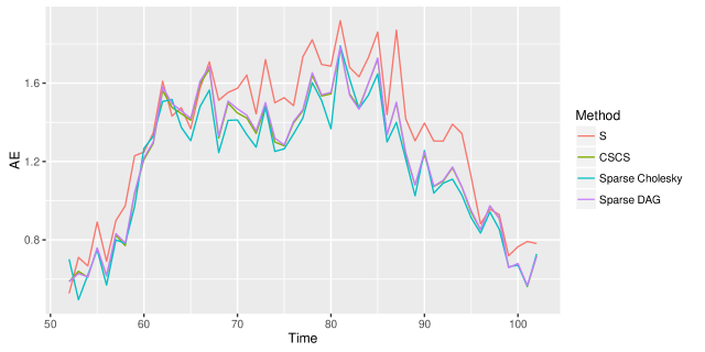
Figure 6: Average Absolute Forecast Error with 205 observations in training dataset

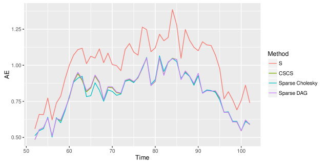
Figure 7: Average Absolute Forecast Error with 150 observations in training dataset

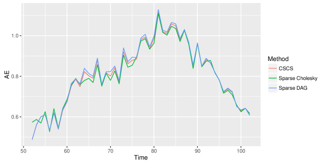
Figure 8: Average Absolute Forecast Error with 100 observations in training dataset

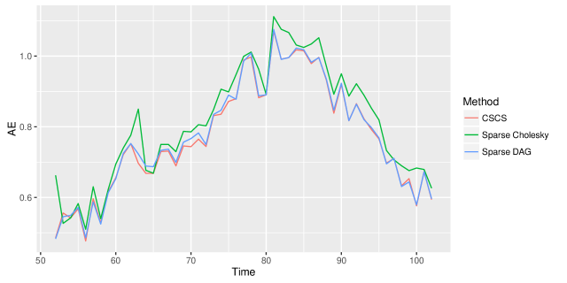
Figure 9: Average Absolute Forecast Error with 75 observations in training dataset

References

[1] J. Friedman, T. Hastie, and R. Tibshirani. Applications of the lasso and grouped lasso to the estimation of sparse graphical models. Technical Report, Department of Statistics, Stanford University, 2010.

[2] K. Khare and B. Rajaratnam. Convergence of cyclic coordinatewise l1 minimization. arxiv, 2014.

[3] K. Khare, S. Oh, and B. Rajaratnam. A convex pseudo-likelihood framework for high dimensional partial correlation estimation with convergence guarantees. Journal of the Royal Statistical Society B, 77:803-825, 2015.

[4] J. Peng, P. Wang, N. Zhou, and J. Zhu. Partial correlation estimation by joint sparse regression models. Journal of the American Statistical Association, 104:735 746, 2009.

[5] M .Rudelson and R. Vershynin. Hanson-Wright inequality and sub-gaussian concentration. Electronic Communications in Probability, 18:1-9, 2013.

References

- [1] O. Banerjee, L. El Ghaoui, and A. D’Aspremont. Model selection through sparse maximum likelihood estimation for multivariate gaussian or binary data. The Journal of Machine Learning Research, 9:485–516, 2008.
- [2] P. Dellaportas and M. Pourahmadi. Cholesky-garch models with applications to finance. Stat. Comput, 22:849–855, 2012.
- [3] T. Fawcett. An introduction to roc analysis. Pattern Recognition Letters, 27(8):861– 874, 2006.
- [4] J. Friedman, T. Hastie, and R. Tibshirani. Regularization paths for generalized linear models via coordinate descent. Journal of Statistical Software, 33:1–22, 2008.
- [5] J. Friedman, T. Hastie, and R. Tibshirani. Sparse inverse covariance estimation with the graphical lasso. Biostatistics, 9:432–441, 2008.
- [6] J. Friedman, T. Hastie, and R. Tibshirani. Applications of the lasso and grouped lasso to the estimation of sparse graphical models. Technical Report, Department of Statistics, Stanford University, 2010.
- [7] W. J. Fu. Penalized regressions: The bridge versus the lasso. Journal of Computational and Graphical Statistics, 7:397–416, 1998.
- [8] C-J. Hsieh, M. A. Sustik, I. S. Dhillon, and P. Ravikumar. Sparse inverse covariance matrix estimation using quadratic approximation. Advances in Neural Information Processing Systems, 24, 2011.
- [9] J. Huang, N. Liu, M. Pourahmadi, and L. Liu. Covariance selection and estimation via penalised normal likelihoode. Biometrika, 93:85–98, 2006.
- [10] K. Khare, S. Oh, and B. Rajaratnam. A convex pseudo-likelihood framework for high dimensional partial correlation estimation with convergence guarantees. Journal of the Royal Statistical Society B, 2014.
- [11] K. Khare and B. Rajaratnam. Convergence of cyclic coordinatewise l1 minimization. Preprint, Department of Statistics, Stanford University, 2014.
- [12] E. Levina, A. Rothman, and J. Zhu. Sparse estimation of large covariance matrices via a nested lasso penalty. Annals of Applied Statistics, 2:245–263, 2008.
- [13] H. Massam, D. Paul, and B. Rajaratnam. Penalized empirical risk minimization using a convex loss function and penalty. unpublished manuscript, 2007.
- [14] R. Mazumder and T. Hastie. Exact covariance thresholding into connected components for large-scale graphical lasso. The Journal of Machine Learning Research, 13:781–794, 2012.
- [15] N. Meinshausen and P. Buhlmann. High dimensional graphs and variable selection with the lasso. Annals of Statistics, 34:1436–1462, 2006.
- [16] S. Oh, O. Dalal, K. Khare, and B. Rajaratnam. Optimization methods for sparse pseudo-likelihood graphical model selection. Proceedings of Neural Information Processing Systems, 2014.
- [17] V. I. Paulsen, S. C. Power, and R. R. Smith. Schur products and matrix completions. J. Funct. Anal., 85:151–178, 1989.
- [18] J. Peng, P. Wang, N. Zhou, and J. Zhu. Partial correlation estimation by joint sparse regression models. Journal of the American Statistical Association, 104:735–746, 2009.
- [19] B. Rajaratnam and J. Salzman. Best permutation analysis. Journal of Multivariate Analysis, 121:193–223, 2013.
- [20] A. Rothman, E. Levina, and J. Zhu. A new approach to cholesky-based covariance regularization in high dimensions. Biometrika, 97:539–550, 2010.
- [21] K. Sachs, O. Perez, D. Pe’er, D. Lauffenburger, and G. Nolan. Causal protein-signaling networks derived from multiparameter single-cell data. Science, 308(5721):504–6, 2003.
- [22] H. Shen and J. Z. Huang. Analysis of call center arrival data using singular value decomposition. Appl. Stoch. Models Bus. and Ind., 21:251–63, 2005.
- [23] A. Shojaie and G. Michailidis. Penalized likelihood methods for estimation of sparse high-dimensional directed acyclic graphs. Biometrika, 97:519–538, 2010.
- [24] M. Smith and R. Kohn. Parsimonious covariance matrix estimation for longitudinal data. Journal of the American Statistical Association, 97:1141–1153, 2002.
- [25] W. B. Wu and M. Pourahmadi. Nonparametric estimation of large covariance matrices of longitudinal data. Biometrika, 90:831–844, 2003.
- [26] G. Yu and J. Bien. Learning local dependence in ordered data. arXiv:1604.07451, 2016.