Vertical stability of circular orbits in relativistic razor-thin disks

Abstract

During the last few decades, there has been a growing interest in exact solutions of Einstein equations describing razor-thin disks. Despite the progress in the area, the analytical study of geodesic motion crossing the disk plane in these systems is not yet so developed. In the present work, we propose a definite vertical stability criterion for circular equatorial timelike geodesics in static, axially symmetric thin disks, possibly surrounded by other structures preserving axial symmetry. It turns out that the strong energy condition for the disk stress-energy content is sufficient for vertical stability of these orbits. Moreover, adiabatic invariance of the vertical action variable gives us an approximate third integral of motion for oblique orbits which deviate slightly from the equatorial plane. Such new approximate third integral certainly points to a better understanding of the analytical properties of these orbits. The results presented here, derived for static spacetimes, may be a starting point to study the motion around rotating, stationary razor-thin disks. Our results also allow us to conjecture that the strong energy condition should be sufficient to assure transversal stability of periodic orbits for any singular timelike hypersurface, provided it is invariant under the geodesic flow.

I Introduction

Many discoidal systems can be modeled in a first approximation as axisymmetric structures. Such systems include disk galaxies (lenticular, barred and spirals) Binney and Tremaine (2008); van der Kruit and Freeman (2011) and accretion disks around black holes and other compact objects Abramowicz and Fragile (2013); Karas et al. (2004); Semerák (2002). In all of these systems, the majority of the orbits of small objects are nearly circular and equatorial (e.g. Sofue and Rubin (2001)), and hence studying the stability of such orbits is specially relevant. Particularly, precise stability criteria for these situations are of great interest. The study of axially symmetric structures in General Relativity (GR) began in 1966 with the work of Papapetrou Papapetrou (1966) on axially symmetric vacuum solutions. Exact solutions for the Einstein equations representing thin disks without radial pressure were first proposed by Morgan and Morgan Morgan and Morgan (1969, 1970). The first applications of the theory of distributions to curved spacetimes representing razor-thin disks of self-gravitating matter were proposed in Bonnor and Sackfield (1968); Voorhees (1972), together with an initial study of the stability of circular geodesics Voorhees (1972). The stability of circular geodesics in smooth axially symmetric stress-energy distributions was first considered in Bardeen (1970), in which some remarks about their vertical stability in the limit of an infinitesimally thin disk are presented. During the last decades, many exact solutions representing thin disks were obtained, both in GR (see for example Bičák et al. (1993); González and Letelier (1999); Lemos and Letelier (1994); Letelier and Oliveira (1987); Semerák et al. (1999a, b); Vogt and Letelier (2003); Ramos-Caro et al. (2012) and the reviews Karas et al. (2004); Semerák (2002)) and in modified theories of gravity Coimbra-Araújo and Letelier (2007); Vieira and Letelier (2014), mainly based on the formalism of distribution-valued curvature tensors proposed by Taub Taub (1980). For razor-thin disks, such an approach is consistent with the results about distributional sources in general relativity obtained by Geroch and Traschen Geroch and Traschen (1987), which provide an adequate framework to deal with distribution-valued curvature tensors with support on spacetime hypersurfaces.

The stability of circular geodesics in smooth axially symmetric spacetimes is usually analyzed by considering the geodesic deviation equation (e.g. Shirokov (1973)). Radial stability can also be analyzed by the relativistic generalization of Rayleigh’s criterion Letelier (2003); Abramowicz and Kluźniak (2005); Vieira et al. (2014). Concerning razor-thin disks, extensive numerical studies of the dynamics of timelike geodesic motion were performed in a wide class of spacetimes, including not only razor-thin disks, but also rings surrounding black holes Saa and Venegeroles (1999); Semerák and Suková (2010, 2012); Suková and Semerák (2013); Witzany et al. (2015). Nevertheless, despite the many existing numerical results, the analytical description of motion around these structures is not yet fully developed.

In contrast to the radial stability case, for which essentially the same analysis used for smooth metrics can be employed, vertical stability cannot be studied in the same framework. The presence of a $\delta$-like singularity on the plane of the thin disk Geroch and Traschen (1987); Lemos and Letelier (1994); González and Letelier (1999); Vieira and Letelier (2014); Taub (1980); Vogt and Letelier (2003) prevents the use of the geodesic deviation equation and the corresponding first-order perturbation approach, as first pointed out in Semerák and Žáček (2000). The existing results about vertical stability of circular geodesics in relativistic thin disks consider only particular cases (dust disk, Voorhees (1972)) or are obtained as a limiting case of smooth stress-energy tensors Bardeen (1970); Semerák and Žáček (2000). Although some authors modeled the effects on the geodesic equations due to this $\delta$-like singularity (e.g. Semerák and Žáček (2000)), the resulting vertical stability criterion is not consistent with a distributional source along the equatorial plane of the spacetime.

In the present work, we solve this apparent contradiction. We present a rigorous framework for the vertical stability analysis of timelike circular geodesics in static, axially symmetric razor-thin disks, based on distribution-valued curvature tensors and sources Geroch and Traschen (1987); Taub (1980). Our framework is conceptually very similar to the Newtonian one Vieira and Ramos-Caro (2016, 2015), which we now extend to the GR domain. The paper is organized as follows. Section II has brief revisions on the Hamiltonian formulation for the geodesic flow in axially symmetric, static spacetimes. The rigorous vertical stability conditions are presented in Section III. In Section IV, we discuss the approximate third integral of motion obtained from the adiabatic invariance of the vertical action, as well as its prediction for the orbit’s envelopes. All results are compared in Section V with numerical experiments for several razor-thin disk models. The conclusions and final remarks are presented in Section VI. We use natural units ($c=G=1$) and the signature $(-,+,+,+)$. Greek indices, which vary from 0 to 3, denote spacetime coordinates; Latin indices, varying from 1 to 3 unless otherwise stated, denote only space coordinates.

II Hamiltonian formulation for the geodesic flow in static, axially symmetric spacetimes

Our experience with the Newtonian case Vieira and Ramos-Caro (2016, 2015) leads us to consider the Hamiltonian formalism for the geodesic flow Ansorg (1998); Bertschinger (1999); Chicone and Mashhoon (2002) as the basis to analyze the vertical stability problem. We exploit the fact that the timelike geodesic equations admit a Hamiltonian formulation in which the spacetime coordinates ($x^{\mu}$) can be interpreted as canonical coordinates, with associated canonical momenta given by $p_{\mu}=g_{\mu\nu}\dot{x}^{\nu}$. All timelike geodesics are assumed to be parametrized by their proper time $\tau$, and the upper dots denote derivatives with respect to $\tau$. The Hamiltonian for timelike geodesics can be written simply as

$$\mathcal{H}(p_{\mu},x^{\mu})=\frac{1}{2}g^{\mu\nu}p_{\mu}p_{\nu},$$ (1)

with the corresponding Hamilton’s equations being fully equivalent to the geodesic equations Ansorg (1998); Chicone and Mashhoon (2002). The Hamiltonian (1) depends on the coordinates $x^{\mu}$ and conjugate momenta $p_{\mu}$, defining a flow in a 8-dimensional phase space. However, it is possible to reduce the dimensionality of the system by defining a new Hamiltonian depending only on $x^{j}$ and $p_{j}$, i.e. the spatial coordinates and associated momenta defined by the timelike vector field foliation, which can facilitate the implementation of concepts and techniques used in the Newtonian framework. Such reduced Hamiltonian is parametrized by the time coordinate $x^{0}$ and leads to a system of equations equivalent to the geodesics derived from (1), but formulated in a 6-dimensional phase space. This can be done by performing the so-called isoenergetic reduction Bertschinger (1999); Chicone and Mashhoon (2002).

Choosing $t=x^{0}$ as the time coordinate for the reduced Hamiltonian, we can adopt a parametrization such that $dt/d\tau>0$ for all timelike geodesics. Solving the constraint $\mathcal{H}=-1/2$ (valid for any timelike geodesic) for the corresponding canonical momentum $p_{0}$, one obtains the effective reduction of the dimensionality of the Hamiltonian system governed by (1). The reduced (and generally time-dependent) Hamiltonian $H=-p_{0}$ Chicone and Mashhoon (2002) will have the the form

$$H(t,p_{i},x^{j})=\frac{g^{0i}p_{i}}{g^{00}}+\bigg{[}\frac{1+\tilde{g}^{ij}p_{i}p_{j}}{(-g^{00})}\bigg{]}^{1/2},$$ (2)

where $\tilde{g}^{ij}$, given by

$$\tilde{g}^{ij}\equiv g^{ij}-\frac{g^{0i}g^{0j}}{g^{00}},$$ (3)

is the inverse of the spatial metric. It is worth pointing out that, in the Newtonian limit, for which $g_{00}=-(1+2\Phi)$, $g^{00}=-(1-2\Phi)$, $g^{i0}=g_{i0}=0$, $\tilde{g}^{ij}=g^{ij}=\delta^{ij}$ and $\Phi$ is the Newtonian gravitational potential, the Hamiltonian of Eq. (2) reduces to

$$H_{N}=\frac{1}{2}\,p^{2}+\Phi+1.$$ (4)

Apart from the constant term, this is the Hamiltonian for Newtonian gravity.

In the present work, we are mainly interested in applying the above formalism to equatorial circular orbits in relativistic static, axially symmetric razor-thin disks. Let us briefly introduce some basic properties of the spacetimes corresponding to such configurations. We begin by considering the general static, axially symmetric metric in cylindrical coordinates ($t,R,\varphi,z$) González and Letelier (1999); Ujevic and Letelier (2004)

$$ds^{2}=-e^{\psi}dt^{2}+e^{\gamma}(R^{2}d\varphi^{2})+e^{\eta}(dR^{2}+dz^{2}),$$ (5)

where $\psi=\psi(R,z)$, $\gamma=\gamma(R,z)$ and $\eta=\eta(R,z)$. Additionally, we assume that the system has reflection symmetry with respect to $z=0$ (equatorial plane), $g_{\mu\nu}(R,-z)=g_{\mu\nu}(R,z)$, along with the conditions ensuring the existence of a razor-thin disk on the equatorial plane: $\partial g_{\mu\nu}/\partial|z|\big{|}_{z=0}\neq 0$. In this case, the isoenergetically reduced Hamiltonian (2) can be cast as

$$H=\bigg{[}e^{\psi-\eta}(p_{R}^{2}+p_{z}^{2})+V_{\rm eff}(R,z)\bigg{]}^{1/2},$$ (6)

where the effective potential $V_{\rm eff}$ is given by

$$V_{\rm eff}=e^{\psi}\bigg{(}1+\frac{L_{z}^{2}}{R^{2}e^{\gamma}}\bigg{)}.$$ (7)

The conserved quantity $L_{z}\equiv p_{\varphi}$ is the $z$-component of the relativistic angular momentum. The reduced Hamiltonian flow now evolves in a 4-dimensional phase space $(p_{R},p_{z},R,z)$,

$$\frac{dp_{i}}{dt}=-\frac{\partial H}{\partial x^{i}},\qquad\frac{dx^{i}}{dt}=\frac{\partial H}{\partial p_{i}},\qquad i=R,z.$$ (8)

Timelike circular geodesics correspond to the fixed point

$$\xi_{o}=(p_{R}=0,\,p_{z}=0,\,R=R_{o},\,z=0),$$ (9)

for which

$$\frac{\partial V_{\rm eff}}{\partial R}=0.$$ (10)

Solving Eq. (10) for $L_{z}$, we obtain the specific angular momentum of a massive test particle moving on an equatorial circular geodesic with radius $R$

$$L_{z}(R)=R^{2}e^{\gamma}\sqrt{\frac{(e^{\psi})_{,R}}{e^{\psi}(R^{2}e^{\gamma})_{,R}-R^{2}e^{\gamma}(e^{\psi})_{,R}}}.$$ (11)

This result is in accordance with the expression obtained by Vogt and Letelier Vogt and Letelier (2003) for isotropic metrics and with the general expression presented in Letelier (2003); Vieira et al. (2014).

III Vertical stability

The Hamiltonian (6) is a Lyapunov function (an integral of motion, indeed) for the reduced flow (8). Therefore, a sufficient condition for Lyapunov stability of a fixed point $\xi$ of the flow (8) is that $\xi$ is a (strict) local minimum of $H$. For the case of equatorial circular orbits, since $e^{\psi-\eta}>0$, it follows from the expression of $H$ [Eq. (6)] that $\xi_{o}$ given by (9) is Lyapunov stable if the corresponding point in the meridional plane $(R,z)$, $(R_{o},0)$, is a (strict) local minimum of $V_{\rm eff}$ (for a proof of this result in the context of classical mechanics, see Arnol’d (1989)). Since this result depends only on the continuity of the Hamiltonian (and not on its smoothness, see Arnol’d (1989)), it remains valid when we introduce a razor-thin disk at the equatorial plane. In this case, the Lyapunov stability condition is equivalent to

$$\frac{\partial V_{\rm eff}}{\partial|z|}(R_{o},0)>0,$$ (12a)

$$\frac{\partial^{2}V_{\rm eff}}{\partial R^{2}}(R_{o},0)>0.$$ (12b)

We can interpret Eqs. (12a) and (12b), respectively, as vertical and radial stability conditions. From Eqs. (7) and (11) we obtain

$$\frac{\partial^{2}V_{\rm eff}}{\partial R^{2}}\bigg{|}_{(R_{o},0)}=\frac{(e^{\psi})_{,R}}{L_{z}^{2}}\frac{dL_{z}^{2}}{dR},$$ (13)

the well-known generalization of Rayleigh’s radial stability criterion Letelier (2003); Vieira et al. (2014). In order to avoid repulsive forces, we must consider only regions where $(e^{\psi})_{,R}>0$ Vieira et al. (2014).

Let us now focus on the vertical stability of timelike circular geodesics. Consider a razor-thin disk surrounded by an axially symmetric matter distribution, also symmetric with respect to the equatorial plane. The vertical stability criterion (12a) gives us

$$\frac{\partial V_{\rm eff}}{\partial|z|}\bigg{|}_{z=0}=e^{\psi}\bigg{\{}\frac{\partial\psi}{\partial|z|}+\frac{L_{z}^{2}}{R^{2}e^{\gamma}}\Big{(}\frac{\partial\psi}{\partial|z|}-\frac{\partial\gamma}{\partial|z|}\Big{)}\bigg{\}}>0,$$ (14)

with the right-hand side evaluated at $z=0$. By our experience with the Newtonian case Vieira and Ramos-Caro (2016, 2015), we would expect that the above expression could be related to the matter-energy distribution of the disk. In fact, we show below that the vertical stability criterion (14) is related to the strong energy condition of the disk fluid. Before that, let us briefly review the basic features of the stress-energy tensor associated to the razor-thin disk.

III.1 Stress-energy tensor of a razor-thin disk

The stress-energy tensor of a system containing a razor-thin disk is given by

$$T^{\mu}_{\ \nu}=Q^{\mu}_{\ \nu}\hat{\delta}(z)+D^{\mu}_{\ \nu},$$ (15)

where $Q^{\mu}_{\ \nu}\hat{\delta}(z)$ corresponds to the razor-thin disk and $D^{\mu}_{\ \nu}$ to the smooth matter distribution surrounding it. Also, $\hat{\delta}(z)$ is the Dirac delta distribution in curved spacetimes, given by (see Vieira and Letelier (2014); Taub (1980)) $\hat{\delta}(z)\equiv\delta(z)/\sqrt{g_{zz}}$, where $\delta(z)$ is the usual Dirac delta distribution (in a flat spacetime), which is related with the Heaviside “step function”, $\theta(z)$, by the known expression $\delta(z)=\theta_{,z}$. One has Taub (1980)

$$\sqrt{g_{zz}}\,\hat{\delta}(z)=\theta_{,z},\qquad\theta(z)=\begin{cases}1,&z>0,\\ 1/2,&z=0,\\ 0,&z<0.\end{cases}$$ (16)

Since $\theta$ does not depend on the spacetime metric, we can write, in this adapted coordinate system,

$$\theta_{,\mu}(z)=\sqrt{g_{zz}}\,\delta_{\mu}^{z}\,\hat{\delta}(z),$$ (17)

where $\delta_{\mu}^{z}$ stands for the normal vector $n_{\mu}$, associated with the razor-thin disk: $n_{\mu}\equiv\partial z/\partial x^{\mu}=\delta_{\mu}^{z}.$ Since $n^{\alpha}n_{\alpha}=g^{zz}$, we have

$$\theta_{,\mu}=\frac{1}{\sqrt{n^{\alpha}n_{\alpha}}}\,n_{\mu}\hat{\delta},$$ (18)

indeed a different expression from that presented in Taub (1980). We will show now that the above expression for $\theta_{,\mu}$ is in fact the correct one, which leads to a modification of the stress-energy tensor of the disk, in comparison to the ones considered in Taub (1980); Lemos and Letelier (1994); González and Letelier (1999); Vogt and Letelier (2003); Vieira and Letelier (2014). First, let us note that $\theta$ does not depend on the particular choice $f(z)$ (instead of $z$) used to describe the thin disk. If $f(z)$ is an increasing function of $z$ with $f(0)=0$, then the corresponding Heaviside function $\theta_{f}$, Eq. (47), satisfies $\theta_{f}=\theta$. Therefore, $\theta_{,\mu}$ cannot depend on the choice of $f$. The normal vector associated with the function $f$ is $\tilde{n}_{\mu}=\partial f/\partial x^{\mu}$ Taub (1980), with norm $\tilde{n}^{\alpha}\tilde{n}_{\alpha}=\big{(}f^{\prime}(z)\big{)}^{2}n^{\alpha}n_{\alpha}$. It follows that ${\sqrt{n^{\alpha}n_{\alpha}}\tilde{n}_{\mu}=}{\sqrt{\tilde{n}^{\alpha}\tilde{n}_{\alpha}}}n_{\mu},$ and from the definition of the delta distribution, $\hat{\delta}$ does not depend on $f$, so we have that neither does $\theta_{,\mu}$, as expected.

The argument used here for razor-thin disks can be extended to an arbitrary timelike singular hypersurface in a curved spacetime, and the result is that the correct expression for $\theta_{,\mu}$ is still given by Eq. (18) (see Appendix A). This correction leads to an stress-energy tensor of the form [see Eq. (15)]

$$Q_{\mu}^{\ \nu} = \frac{1}{16\pi}\frac{1}{\big{(}n^{\lambda}n_{\lambda}\big{)}^{1/2}}\Big{\{}b_{\mu}^{\ \sigma}n_{\sigma}n^{\nu}-b_{\sigma}^{\ \sigma}n_{\mu}n^{\nu}-b_{\mu}^{\ \nu}n_{\sigma}n^{\sigma}+$$ (19)

$$+b_{\sigma}^{\ \nu}n_{\mu}n^{\sigma}+\delta_{\mu}^{\nu}\big{(}b_{\sigma}^{\ \sigma}n_{\alpha}n^{\alpha}-b_{\alpha}^{\ \sigma}n_{\sigma}n^{\alpha}\big{)}\Big{\}},$$

(compare to Barrabès (1989), eq. 17, and Taub (1980), eqs. 2.11–2.14), where the coefficients $b_{\mu\nu}$ are given by Eq. (50)

$$[g_{\mu\nu,\alpha}]\equiv b_{\mu\nu}n_{\alpha},$$ (20)

and $b^{\mu}_{\ \nu}=b_{\alpha\nu}g^{\mu\alpha}$, $b^{\mu\nu}=g^{\alpha\nu}b^{\mu}_{\ \alpha}$ (see Appendix A). For the case of a razor-thin disk, with the simplest choice $f(z)=z$, we have $n_{\mu}=\delta_{\mu}^{z}$ and

$$b_{\mu\nu}=g_{\mu\nu,z}\Big{|}_{z=0^{+}}-g_{\mu\nu,z}\Big{|}_{z=0^{-}}=2\frac{\partial g_{\mu\nu}}{\partial|z|}\bigg{|}_{z=0},$$ (21)

The stress-energy tensor of the disk is therefore given by

$$Q^{\mu}_{\ \nu} = \frac{\sqrt{g_{zz}}}{16\pi}\bigg{\{}b^{\mu z}\delta^{z}_{\nu}-b^{zz}\delta^{\mu}_{\nu}+g^{\mu z}b^{z}_{\ \nu}-$$ (22)

$$-g^{zz}b^{\mu}_{\ \nu}+b^{\alpha}_{\ \alpha}(g^{zz}\delta^{\mu}_{\nu}-g^{\mu z}\delta^{z}_{\nu})\bigg{\}}.$$

The formalism introduced here elucidates the rather artificial distinction in the literature between the “true” and the “physical” stress-energy tensor of a relativistic razor-thin disk González and Letelier (1999); Lemos and Letelier (1994); Vogt and Letelier (2003); Vieira and Letelier (2014). We see that the really relevant quantity is $Q^{\mu}_{\ \nu}$ [Eqs. (19), (22)], which corresponds indeed to the “physical” stress-energy tensor in the references above.

Note that it follows immediately from Eq. (22) that

$$Q^{z}_{\ z}=0.$$ (23)

Also, substituting the components of the metric (5) in (22), we obtain the nonzero components of $Q_{\mu}^{\ \nu}$:

$$Q^{t}_{\ t}=\frac{e^{-\eta/2}}{8\pi}\bigg{\{}\frac{\partial\gamma}{\partial|z|}+\frac{\partial\eta}{\partial|z|}\bigg{\}}\bigg{|}_{z=0},$$ (24a)

$$Q^{\varphi}_{\ \varphi}=\frac{e^{-\eta/2}}{8\pi}\bigg{\{}\frac{\partial\psi}{\partial|z|}+\frac{\partial\eta}{\partial|z|}\bigg{\}}\bigg{|}_{z=0},$$ (24b)

$$Q^{R}_{\ R}=\frac{e^{-\eta/2}}{8\pi}\bigg{\{}\frac{\partial\psi}{\partial|z|}+\frac{\partial\gamma}{\partial|z|}\bigg{\}}\bigg{|}_{z=0}.$$ (24c)

From (24), we have $Q^{\mu}_{\ \nu}={\rm diag}(-\sigma,P_{R},P_{\varphi},0),$ where $\sigma$ is the energy surface density of the disk and $P_{R},P_{\varphi}$ are its principal pressures in the $R$- and $\varphi$- directions (see González and Letelier (1999)). Inverting relations (24), we finally obtain

$$\frac{\partial\psi}{\partial|z|}\bigg{|}_{z=0}=4\pi e^{\eta/2}(\sigma+P_{\varphi}+P_{R}),$$ (25)

$$\frac{\partial\psi}{\partial|z|}\bigg{|}_{z=0}-\frac{\partial\gamma}{\partial|z|}\bigg{|}_{z=0}=8\pi e^{\eta/2}(\sigma+P_{\varphi}).$$ (26)

III.2 The criterion for vertical stability

The necessary and sufficient condition for vertical stability of an equatorial circular geodesic of radius $R=R_{o}$ is given by Eq. (14). We now write it in terms of the underlying stress-energy tensor. This condition is obtained after substituting Eqs. (25) and (26) in (14), evaluated at ($R_{o},0$):

$$\frac{\partial V_{\rm eff}}{\partial|z|}\bigg{|}_{(R_{o},0)} = 4\pi e^{\psi+\eta/2}\Big{\{}\big{(}\sigma+P_{\varphi}+P_{R}\big{)}+$$ (27)

$$+2\frac{L_{z}^{2}}{R^{2}e^{\gamma}}\big{(}\sigma+P_{\varphi}\big{)}\Big{\}}\bigg{|}_{(R_{o},0)}>0.$$

Therefore, a sufficient condition for vertical stability of a circular geodesic of radius $R_{o}$ in the equatorial plane is

$$\begin{cases}\sigma+P_{\varphi}+P_{R}>0,\\ \\ \sigma+P_{\varphi}>0\end{cases}$$ (28)

at $R=R_{o}$, which is the key result of this work: The strong energy condition for the disk fluid (see Hawking and Ellis (2008); Wald (1984)) suffices to assure vertical stability of all circular timelike geodesics in a static razor-thin disk surrounded by a distribution of matter with the same symmetries. Such a statement, or the more general condition (14) or (27), formalizes, in the context of the theory of distribution-valued stress-energy tensors Geroch and Traschen (1987); Taub (1980), the previous results Bardeen (1970); Voorhees (1972) about the vertical stability of circular geodesics in the presence of a razor-thin disk.

When restricted to some cases of interest, conditions (28) adopt a quite simplified form. For example, in the case of an isotropic metric ($\gamma=\eta$), the disk has an isotropic pressure, i.e. $P_{\varphi}=P_{R}\equiv P$ [see Eqs. (24b) and (24c)], and relations (28) reduce to

$$\mbox{Isotropic Metric}\>\>\rightarrow\qquad\begin{cases}\sigma+2P>0,\\ \\ \sigma+P>0.\end{cases}$$

For a Weyl metric ($\gamma=-\psi$) we have $P_{R}=0$ [from Eq. (24c)]. In this case, the vertical stability conditions (28) reduce to

$$\mbox{Weyl Metric}\>\>\rightarrow\qquad\sigma+P_{\varphi}>0.$$

In the case of a dust thin disk ($\gamma=\eta=-\psi$), for which $P_{R}=P_{\varphi}=0$, we have

$$\mbox{Dust Thin Disk}\>\>\rightarrow\qquad\sigma>0.$$

We close this section by briefly mentioning that, writing (27) as

$$\frac{\partial V_{\rm eff}}{\partial|z|}\bigg{|}_{(R_{o},0)} = 4\pi e^{\psi+\eta/2}\Big{\{}\Big{(}1+\frac{L_{z}^{2}}{R^{2}e^{\gamma}}\Big{)}\big{(}\sigma+P_{\varphi}+P_{R}\big{)}+$$ (29)

$$+\frac{L_{z}^{2}}{R^{2}e^{\gamma}}\big{(}\sigma+P_{\varphi}-P_{R}\big{)}\Big{\}}\bigg{|}_{(R_{o},0)},$$

we can obtain another sufficient condition for vertical stability of the orbits: $\sigma+P_{\varphi}>|P_{R}|$. This criterion, however, is more stringent than (28), of which is a particular case.

IV Approximate third integral of motion

Following the same procedure applied to the Newtonian case Vieira and Ramos-Caro (2016, 2015), we obtain an approximate third integral of motion $I_{3}$ and the amplitude of the envelope $Z(R)$ of a nearly equatorial orbit, by considering an approximate separable Hamiltonian near the stable circular orbit of radius $R_{o}$ and exploring the adiabatic invariance of the action variables (under the assumption of slow $R$-variations). We keep fixed the total energy $H=E$ and the $z$-component of the angular momentum $L_{z}$.

IV.1 Motion near a stable circular orbit

The approximate Hamiltonian near a circular orbit of radius $R_{o}$ is, to first order in $|z|$ and for small momenta, given by

$$H^{2}\approx A(R_{o})\big{(}p_{R}^{2}+p_{z}^{2}\big{)}+V_{\rm eff}(R,0)+\frac{\partial V_{\rm eff}}{\partial|z|}(R_{o},0)|z|,$$ (30)

where $A(R_{o})\equiv e^{\psi-\eta}(R_{o},0)>0$ and all higher-order terms proportional to $|z|R$, $|z|R^{2}$ and so on were discarded. Notice that $H^{2}$ is separable, and therefore $H$ is integrable in these coordinates. In particular, by introducing

$$g(R_{o})\equiv\frac{\partial V_{\rm eff}}{\partial|z|}(R_{o},0),$$ (31)

then the quantity

$$H_{z}^{2}\equiv A(R_{o})p_{z}^{2}+g(R_{o})|z|$$ (32)

is conserved for the Hamiltonian (30). The corresponding generating function for the vertical action-angle coordinates is given by

$$S_{z}=\frac{1}{\sqrt{A(R_{o})}}\int^{z}\sqrt{E_{z}^{2}-g(R_{o})|z|}dz,$$ (33)

and the corresponding vertical action variable, in terms of the amplitude of motion $Z\equiv z_{max}$, is

$$J_{z}=\frac{4g_{R_{o}}^{1/2}}{3\pi\sqrt{A(R_{o})}}Z^{(3/2)}.$$ (34)

Now, from Eq. (27),

$$g(R_{o}) = 4\pi e^{\psi+\eta/2}\Big{\{}\big{(}\sigma+P_{\varphi}+P_{R}\big{)}+$$

$$+2\frac{L_{z}^{2}}{R^{2}e^{\gamma}}\big{(}\sigma+P_{\varphi}\big{)}\Big{\}}\bigg{|}_{(R_{o},0)}$$

and defining $\tilde{g}(R_{o})\equiv g(R_{o})/A(R_{o})$, we finally get

$$J_{z}=\frac{4\sqrt{\tilde{g}(R_{o})}}{3\pi}Z^{(3/2)},$$ (35)

which is an approximate adiabatic invariant for our system.

IV.2 Adiabatic invariance of $J_{z}$

As in the Newtonian case Vieira and Ramos-Caro (2016, 2015), the approximate adiabatic invariance of $J_{z}$ implies that the shape of nearly equatorial orbits is determined by the envelope satisfying

$$\frac{Z(R)}{Z(R^{\prime})}=\bigg{(}\frac{\tilde{g}(R^{\prime})}{\tilde{g}(R)}\bigg{)}^{1/3},$$ (36)

where

$$\tilde{g}(R) = 4\pi e^{3\eta/2}\Big{\{}\big{(}\sigma+P_{\varphi}+P_{R}\big{)}+$$ (37)

$$+2\frac{L_{z}^{2}}{R^{2}e^{\gamma}}\big{(}\sigma+P_{\varphi}\big{)}\Big{\}}\bigg{|}_{z=0},$$

provided the period $T_{z}$ of vertical oscillations is smaller than the period $T_{R}$ of radial oscillations. The corresponding third integral of motion (in addition to $H$ and $L_{z}$) is given at the orbit’s envelope by $I_{3}=Z(R)[\tilde{g}(R)]^{1/3}$, where $\tilde{g}$ is given by Eq. (37). The vertical amplitude $Z(R)$ depends implicitly on the phase-space coordinates, $Z=Z(p_{R},p_{z},R,z)$. In terms of these coordinates, $I_{3}$ can be written as

$$I_{3}=\frac{1}{\big{[}\tilde{g}(R)\big{]}^{2/3}}\bigg{[}\,p_{z}^{2}+\tilde{g}(R)|z|\,\bigg{]},$$ (38)

an expression similar to the Newtonian case Vieira and Ramos-Caro (2016).

At this point, it is worth comparing the GR predictions for the shape of the envelopes (36) and for the approximate third integral (38) with the Newtonian equivalent ones. Typically, GR razor-thin disks present orbits whose shape depends also on its angular momentum and on its principal pressures, rather than solely on its surface density. There is also a dependence on the metric components. Therefore, the surrounding halo can affect the shape of nearly equatorial orbits through the influence on these metric components. These are purely relativistic effects, a direct consequence of the nonlinearity of Einstein’s field equations. Although the knowledge of only the physical properties of the thin disk is sufficient to guarantee vertical stability of circular orbits (once the strong energy condition is satisfied), it is not enough to determine the shape of nearly equatorial orbits: We must have information about the surrounding matter (or, equivalently, about the metric components).

V Numerical experiments

We have tested our results against exhaustive numerical experiments. In this Section, we present some typical results for relativistic razor-thin disk models. Specifically, we compare the envelopes of the low-amplitude orbits with the prediction of the adiabatic approximation [see Eq. (36)] and, most importantly, check the validity of formula (38) for the third integral of motion. All cases we considered correspond to spacetimes with an isotropic metric of the form

$$ds^{2}=-\biggl{(}\frac{1-f}{1+f}\biggr{)}^{2}dt^{2}+(1+f)^{4}(dR^{2}+dz^{2}+R^{2}d\varphi^{2}),$$ (39)

where $f$ is some function of $R$ and $z$, which determines each particular model. The properties of a spacetime given by (39) are well known. In particular, according to (24), we have for such spacetimes

$$\sigma=-\frac{1}{\pi(1+f)^{3}}\frac{\partial f}{\partial|z|},\ \ \ P=\bigg{(}\frac{1}{4(1-f)}-\frac{1}{2}\bigg{)}\sigma,$$ (40)

where $P=P_{\varphi}=P_{R}$. For all metrics with $\partial f/\partial|z|<0$, vertical stability is assured. Incidentally, all the usual energy conditions for the disk fluid are also verified in this case for the exterior region of (39) ($f<1$).

For the sake of comparison with the Newtonian limit Vieira and Ramos-Caro (2016), it is convenient to consider the quantity

$$\Delta E^{2}=\frac{E^{2}-E^{2}_{\rm min}}{E^{2}_{\rm min}}$$ (41)

which measures the difference between the particle’s energy and the minimum of the effective potential, $E^{2}_{\rm min}$. Let us now consider four explicit examples.

V.1 Vogt-Letelier disks

The first model we consider is a GR extension, due to Vogt and Letelier Vogt and Letelier (2003), of the so-called Kuzmin disk in the Newtonian context. It consists basically on a razor-thin disk in the equatorial plane of an external vacuum (Schwarzschild) field. In this case, one has

$$f(R,z)=\frac{m}{2\sqrt{R^{2}+(|z|+a)^{2}}}.$$ (42)

The disk is defined by the quantities $m$ and $a$, both positive parameters, whereas the orbits are specified by the constants of motion, $E$ and $L_{z}$, besides the initial conditions.

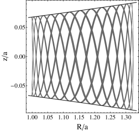
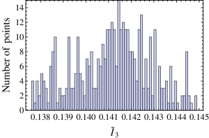
Figure 1: Top, left: Orbit in the meridional plane $(R,z)$ for the Vogt-Letelier disk with $m/a=1$. It has initial conditions $R_{o}/a=1$, $P_{R}=0$ and $z_{o}/a=10^{-8}$. The values of angular momentum and energy are $L_{z}/a=2.2$, $E^{2}=0.6$, giving $\Delta E^{2}\approx 0.04$. The ratio between the vertical and radial average periods is $T_{z}/T_{R}\approx 0.2$. It was calculated from the peaks in the time series of $z(t)$ and $R(t)$. The predicted envelopes from Eq. (36) are shown by black lines. In our choice, the predicted and numerically calculated envelopes have the same value at the upper point of the zero-velocity curve. The predicted envelopes from Eq. (36) are shown by black lines. They agree with the envelopes of the numerically integrated orbits. Top, right: Poincaré section in the surface of constant energy and angular momentum given by the orbit’s parameters, with $R/a=1.2$. The consequents of the orbits are calculated for both $P_{R}>0$ and $P_{R}<0$ and are given by black dots, whereas the prediction from the average value $\tilde{I}_{3,\rm mean}=a^{-2/3}I_{3,\rm mean}=0.141$ is given by the solid black line. We see that Eq. (38) is a good description for the approximate third integral in low-amplitude orbits. Bottom, left: Time series of $\tilde{I}_{3}(t)=a^{-2/3}I_{3}(t)$, given by Eq. (38). It shows small spread along time evolution. Bottom, right: Histogram for $\tilde{I}_{3}(t)$.

As in the Newtonian case Vieira and Ramos-Caro (2016), where we have obtained for the Kuzmin disk unexpectedly large regions in which the approximate third integral is valid, we also note that for Vogt-Letelier disks with moderate density profiles ($a/m\gg 1/2$) the same situation occurs. Varying the parameters $a$, $E$ and $L_{z}$, it is possible to investigate whether the aforementioned approximate third integral is valid along the whole parameter space. We find that Eq. (38) is always valid along the disk if we consider small enough deviations from circular motion, however its range of validity depends heavily on the parameters. In particular, for stronger gravity ($a/m\gtrsim 1/2$), the adiabatic approximation has a rather limited extension near the center of the disk (low angular momentum). Typically, if the energy of the perturbed orbit is small, the prediction from (38) holds, but once we go to higher values of energy (or higher radial excursions of the particle) the prediction for the envelopes is poorer. We present in Fig. 1 a typical disk-crossing orbit oscillating near the equatorial plane and far from the disk center. In this case the period of $R$-oscillations is approximately ten times the period of vertical oscillations. Similar features appear in situations including a halo, but we have to take into account that the volume distribution can introduce significant deviations from the prediction of Eq. (38). This is the case of the next considered disks.

V.2 Kuzmin disk and a Plummer halo

In spherical coordinates, the Plummer potential is defined as $\phi=-GM[r^{2}+b^{2}]^{-1/2}$ Binney and Tremaine (2008), so a general relativistic extension of a Kuzmin disk immersed in a Plummer halo is obtained by defining

$$f(R,z)=\frac{m}{2\sqrt{R^{2}+(|z|+a)^{2}}}+\frac{M}{2\sqrt{b^{2}+R^{2}+z^{2}}},$$ (43)

where the constants $m$ (disk mass), $M$ (halo mass), $a$ and $b$ are positive parameters. Let us call this solution “relativistic Kuzmin-Plummer spacetime”. For different combinations of these constants and with the total energy $E$ sufficiently low, we found a variety of orbits well described by Eq. (38), even for the case in which the halo and disk masses are comparable, as in Fig. 2, where $M/m=10^{-1}$. The calculation details are analogous to those of Fig. 1. For lower ratios $M/m$ we obtain a wider range of validity for relation (38). As in the Newtonian case, we find that the validity of (38) decreases as the halo mass increases, especially in regions where $R$ is of the order of $b$ or smaller.

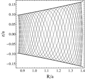
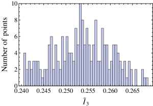
Figure 2: Top, left: Orbit in the meridional plane $(R,z)$ for the relativistic Kuzmin-Plummer spacetime with $m/a=1$, $M/m=0.1$, and $b/a=1$. It has initial conditions $R_{o}/a=1.4$, $P_{R}=0$ and $z_{o}/a=10^{-8}$. The values of angular momentum and energy are $L_{z}/a=2.5$, $E^{2}=0.6$ ($\Delta E^{2}\approx 0.08$). For this case, $T_{z}/T_{R}\approx 0.33$. The predicted and numerically calculated envelopes are depicted as in Fig. 1. Again, the agreement is quite satisfactory. Top, right: Poincaré section with $R/a=1.1$, as in Fig. 1. Bottom, left: Time series of $\tilde{I}_{3}(t)=a^{-2/3}I_{3}(t)$, given by Eq. (38). It shows small spread along time evolution. Bottom, right: Histogram for $\tilde{I}_{3}(t)$. The results confirm that Eq. (38) is a good approximate third integral for low-amplitude orbits.

V.3 Disk and halo from Buchdahl solution

Another interesting example of solution that can be interpreted as an axisymmetric disk with a surrounding halo was presented in Vogt and Letelier (2003), starting from Buchdahl’s solution Buchdahl (1964), a spherically symmetric model resembling an Emden polytrope of index 5. It corresponds to

$$f(R,z)=\frac{B}{\sqrt{1+k[R^{2}+(|z|+a)^{2}]}},$$ (44)

where $B$, $k$ and $a$ are positive parameters. We found typically similar results as in the Kuzmin-Plummer spacetime. In particular, the predicted envelopes from (36) are verified with good accuracy for low-amplitude orbits, see Fig. 3 for further details. In this case, all predictions seem to work better for orbits with small amplitudes obtained from an effective potential whose critical point is away from the center of the configuration. However, in this situation one can find values of parameters leading to an effective potential characterized by three critical points, two of them stable and the other one unstable, which is the case of the parameters of Fig. 3. In such conditions, we can find significant deviations between the predictions and the numerical results, if the energy is large enough. This case certainly deserves further investigations since most probably this might be the onset of chaotic behavior in the system.

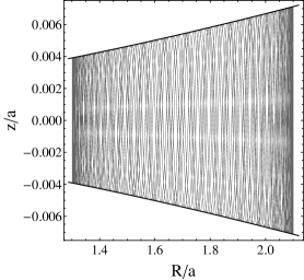
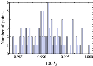
Figure 3: Numerical results for the disk and halo configuration obtained from the Buchdahl solution with $B=1$ and $k/a=2$. The definitions are the same of Figs. 1 and 2. The orbit initial conditions are $R_{o}/a=2.1$, $P_{R}=0$ and $z_{o}/a=10^{-8}$, with $L_{z}/a=5$, $E^{2}=0.92$ ($\Delta E^{2}\approx 0.01$). We have $T_{z}/T_{R}\approx 0.18$ The Poincaré section is calculated for with $R/a=1.4$ and compared with the predictions for $\tilde{I}_{3,\rm mean}=0.01$. $\tilde{I}_{3}(t)$ shows small spread along time evolution.

V.4 Kuzmin-Hernquist spacetime

Deviations from Eq. (38) caused by halo effects can also be seen in the relativistic extension of the so-called Kuzmin-like potentials Hunter (2005), i.e axisymmetric solutions of the form $\phi=\phi(\xi)$, where $\xi=\sqrt{R^{2}+(a+|z|)^{2}}$. It can be shown that these potentials are produced by the combination of a razor-thin disk at $z=0$ and a volume density Hunter (2005). Here we choose $\phi$ with the form of Hernquist potential, i.e. proportional to $[1+(\xi/b)]^{-1}$, and the corresponding relativistic extension is defined by

$$f(R,z)=\frac{\phi_{o}}{2\left[1+b^{-1}\sqrt{R^{2}+(a+|z|)^{2}}\right]},$$ (45)

where $\phi_{o}$, $a$ and $b$ are positive constants. Let us call this solution Kuzmin-Hernquist spacetime. Its results are depicted in Fig. 4. Notice that the envelopes (36) present in this case a non-negligible difference from the actual vertical amplitudes, as well as the predicted surface of section is a bit far from the numerically obtained one.

It is worth noting that the solutions considered in Sec. V.1 and Sec. V.3 are also particular cases of the present family. In all examples, the relativistic extension of the Newtonian gravitational potential $\phi$ was obtained by defining $f=-\phi/2$. The Kuzmin disk corresponds to choosing $\phi=-GM/r$. There is no halo contribution in this case, and the Newtonian gravitational potential is solely due to a razor-thin layer on the equatorial plane. This feature is inherited by the corresponding relativistic extension defined by (42). On the other hand, Eq. (44) is the result of the choice $\phi=-2B/\sqrt{1+kr^{2}}$, which corresponds to the Emden polytrope of order 4, leading to a spheroidal volume distribution with a razor thin disk at $z=0$, similar to situation described by (45). In both cases, we note that as the three-dimensional contribution grows, the prediction of Eq. (38) tends to be less accurate, since it only takes into account the fields calculated at the equatorial plane.

       

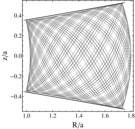
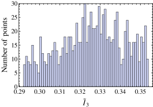
Figure 4: Numerical results for Kuzmin-Hernquist spacetime with $\phi_{o}=1$ and $b=1$. The definitions are the same of Figs. 1 and 2. The orbit initial conditions are $R_{o}/a=1.8$, $P_{R}=0$ and $z_{o}/a=10^{-8}$, with $L_{z}/a=0.74$, $E^{2}=0.6$, ($\Delta E^{2}\approx 0.06$). We have $T_{z}/T_{R}\approx 0.7$. The Poincaré section is calculated for with $R/a=1.4$ and compared with the predictions for $\tilde{I}_{3,\rm mean}=0.326$. $\tilde{I}_{3}(t)$ shows small spread along time evolution.

VI Conclusions

We showed that the necessary and sufficient condition to assure vertical stability of equatorial circular geodesics in relativistic razor-thin disks is $\partial V_{\rm eff}/\partial|z|>0$, evaluated at the disk plane $z=0$ with $L_{z}=L_{z}(R_{o})$. It turns out that the strong energy condition for the singular disk’s stress-energy content suffices to assure the vertical stability of the equatorial circular geodesics. This last result has already been suggested by Bardeen Bardeen (1970) by considering the thin-limit of a thick disk, but without a more rigorous approach based on the theory of distribution-valued stress-energy tensors as done here.

It is worth pointing out that the vertical stability condition obtained here corresponds, in the Newtonian limit, to the expected result $\sigma>0$ Vieira and Ramos-Caro (2016, 2015). Since the strong energy condition can be considered as one of the possible relativistic extensions to the positivity of mass in Newtonian gravity, we may regard our criterion as a natural counterpart in GR of the Newtonian one. On the other hand, the approximated third integral $I_{3}$ obtained in Section IV via the adiabatic approximation is not so directly related to the Newtonian result Vieira and Ramos-Caro (2016, 2015). From Eqs. (36) and (37) we see that, although the Newtonian limit gives us the expected result, the nonlinearity of Einstein’s field equations couples the metric functions and the value of the angular momentum of the orbit to the physical components of the thin-disk fluid. The corresponding third integral in Newtonian gravity (obtained via the adiabatic approximation) depends only on the surface density of the thin disk, whereas in GR this nonlinear coupling makes that the corresponding third integral depends implicitly on the properties of the surrounding matter and on the principal pressures of the disk [see Eqs. (37)–(38)]. Therefore, the only case in which $I_{3}$ is generated solely by the razor-thin disk is when there is no surrounding matter and, hence, the vacuum field equations are verified outside the singular hypersurface.

Our definite criterion obtained here solves a quite old apparent paradox in the literature, since different papers have proposed different vertical stability criteria for circular orbits in the presence of a razor-thin disk Bardeen (1970); Voorhees (1972); Semerák and Žáček (2000); Žáček and Semerák (2002); Semerák (2002); Karas et al. (2004). The results of Bardeen (1970); Voorhees (1972) point in the direction of the proof presented in this paper, whereas the results of Semerák and Žáček (2000); Žáček and Semerák (2002); Semerák (2002); Karas et al. (2004) are mathematically inconsistent and the conclusions derived from them must be reformulated in light of the present approach. Since the stability criterion obtained and the adiabatic invariance analysis are both local, we can extend our formalism to black holes surrounded by razor-thin disks or rings Karas et al. (2004); Lemos and Letelier (1994); Semerák and Žáček (2000); Semerák and Suková (2010, 2012), provided the metric outside the horizon has the form (5) and the orbit does not cross the horizon. In particular, the results obtained in Semerák and Žáček (2000); Žáček and Semerák (2002) about vertical instabilities in the inner part of the Lemos-Letelier disk Lemos and Letelier (1994) (inverted first Morgan and Morgan disk) superposed to a Schwarzschild black hole, as well as the results in section 4 of the same paper (concerning vertical oscillations of orbits in general razor-thin disks), must be reformulated in terms of the vertical stability criterion presented here. It turns out that the inverted first Morgan and Morgan razor-thin disk satisfies the strong energy condition, since this condition for the Weyl metric [Eq. (5) with $\gamma=-\psi$] is equivalent to

$$\frac{\partial\psi}{\partial|z|}\bigg{|}_{z=0}>0$$ (46)

by Eq. (25), which is satisfied along the whole disk (see eq. 32 of Semerák and Žáček (2000) or eq. 10 of Žáček and Semerák (2002)). Thus, the conclusions about the radius of the innermost stable circular orbits (ISCOs) in the “black hole + thin disk” superposition of Semerák and Žáček (2000); Žáček and Semerák (2002) must be reformulated in terms of the new vertical stability criterion. The authors found a maximum value for the ratio between the disk and black-hole masses in order to preserve vertical stability of the circular geodesics when approaching the disk’s inner rim. However, as mentioned in their paper Žáček and Semerák (2002), the above result was obtained neglecting the $\delta(z)$ term. In view of the new framework introduced here, there is no such limitation. The inner-rim circular orbits are vertically stable regardless of the mass of the central black hole or of the disk, and therefore the radius of the ISCO in the system under consideration depends only on the stability under radial perturbations, which was analyzed in Semerák and Žáček (2000). According to the aforementioned analysis, the inner circular orbits of the disk tend to be more stable with growing disk mass, as obtained in Semerák and Záček (2000) for purely equatorial motion, since the only physical quantity to be considered is the radial epicyclic frequency $\kappa$ (the corresponding radial frequencies are shown graphically in Semerák and Žáček (2000)).

According to the results presented here for static razor-thin disks and to the preliminary results of Bardeen (1970) for the stationary case (although without a formal proof), as well as to preliminary computations made by the first author regarding motion crossing spherical thin shells, we conjecture that the strong energy condition for the stress-energy content of a singular timelike hypersurface is a sufficient condition to guarantee “transversal” stablity of the periodic orbits of this hypersurface, provided that this surface is invariant under the timelike geodesic flow. This conjecture will be tested in the future for different spacetimes presenting this characteristic. We also note that, since the reduced Hamiltonian $H$ [Eq. (6)] is a Lyapunov function for the system (8), all stability conclusions are invariant under coordinate transformations which preserve the time coordinate associated with the timelike Killing vector field.

As a final comment, the extension of Eqs. (36)–(38) to three-dimensional disks with flattened density and pressure profiles is not straightforward. One cannot adopt a “vertically integrated” profile (as done in Newtonian gravity; see Vieira and Ramos-Caro (2014)) without a careful examination of the term (37). The difficulty arises from the nonlinear coupling of the metric with the physical components of the disk. Therefore, there is no unique way of extending Eqs. (36)–(38) to thick disks in GR. A more careful analysis is needed in order to compare the possible extensions to three-dimensional structures. This topic will be addressed in future works.

Appendix A Stress-energy tensor for singular hypersurfaces

Let $\mathcal{M}$ be the spacetime manifold and consider a timelike hypersurface $\mathcal{S}$ which splits $\mathcal{M}$ in two parts, i.e., $\mathcal{M}=\mathcal{M}^{+}\cup\mathcal{S}\cup\mathcal{M}^{-}$. Let $\phi:\mathcal{M}\to\mathbb{R}$ be a function such that $\mathcal{S}=\phi^{-1}(0)$, with $0$ a regular value of $\phi$. We choose $\mathcal{M}^{\pm}\equiv\phi^{-1}(\mathbb{R}^{\pm})$. The “Heaviside step function” associated with $\mathcal{M}^{+}$ is given by Taub (1980)

$$\theta(\phi)=\begin{cases}1,&\phi>0,\\ 1/2,&\phi=0,\\ 0,&\phi<0.\end{cases}$$ (47)

Notice that $\theta(\phi)$ does not depend on the particular form of $\phi$, but only on its orientation. The normal vector associated with $\phi$ is given by $n_{\mu}\equiv\partial\phi/\partial x^{\mu}$ Barrabès (1989); Taub (1980), and the unit normal vector associated with the given orientation is

$$t_{\mu}\equiv\frac{1}{\sqrt{n^{\alpha}n_{\alpha}}}n_{\mu}.$$ (48)

We define the “jump” in the derivative of a function $f$ through $\mathcal{S}$ by Taub (1980)

$$[f]_{,\mu}\equiv f^{+}_{,\mu}-f^{-}_{,\mu},$$ (49)

and the jump in the metric derivatives by the coefficients $b_{\mu\nu}$:

$$[g_{\mu\nu,\alpha}]\equiv b_{\mu\nu}n_{\alpha}.$$ (50)

The Dirac delta distribution $\hat{\delta}$ with support on $\mathcal{S}$ is defined by Taub (1980)

$$\int_{\Omega}\hat{\delta}f\sqrt{-g}d^{4}x=\int_{A}fd^{3}V,$$ (51)

where $f:\mathcal{M}\to\mathcal{R}$ is an integrable function and $A=\Omega\cap\mathcal{S}$. Here, $d^{3}V$ stands for the volume element of $S$ induced by the spacetime metric. Contrary to what was stated in Taub (1980), the correct formula for the derivative of the Heaviside function is $\theta_{,\mu}=t_{\mu}\hat{\delta}$, which indeed corresponds to (18). It is clear from the definition of $\theta$ that $\theta_{,\mu}$ should depend neither on the specific form of $\phi$ (since $\theta$ depends only on $\mathcal{S}$) nor on the form of the spacetime metric (since partial differentiation does not depend on the existence of a metric). We can readily see that the above equation for $\theta_{,\mu}$ satisfies both requirements. The corresponding equation given in Taub (1980), however, gives a different result if we choose a different function $\tilde{\phi}$ to describe $\mathcal{S}$ or if we consider a different metric $\tilde{g}$ for the spacetime, maintaining its causal structure.

We can prove that the correct formula for $\theta_{,\mu}$ is indeed (18). Given a compact domain $\Omega\subset\mathcal{M}$ such that $\Omega\cap\mathcal{S}=A$, $\theta_{,\mu}t^{\mu}$ is well defined in $\Omega$ and

$$\int_{\Omega}\theta_{,\mu}t^{\mu}f\sqrt{-g}d^{4}x=\int_{\Omega}\left[(\theta f\zeta^{\mu})_{;\mu}-\theta(f\zeta^{\mu})_{;\mu}\right]\sqrt{-g}d^{4}x$$

$$\quad=\int_{\Omega}\left(\theta f\zeta^{\mu}\right)_{;\mu}\sqrt{-g}d^{4}x-\int_{\Omega^{+}}(f\zeta^{\mu})_{;\mu}\sqrt{-g}d^{4}x,$$ (52)

where $\Omega^{+}\equiv\Omega\cap\mathcal{M}^{+}$ and $\zeta^{\mu}$ is a smooth spacelike vector field satisfying $\zeta^{\mu}=t^{\mu}$ over $\mathcal{S}$. We have that

$$\int_{\Omega^{+}}(f\zeta^{\mu})_{;\mu}\sqrt{-g}d^{4}x\xrightarrow{Vol(\Omega^{+})\to 0}0.$$ (53)

Moreover,

$$\int_{\Omega}\left(\theta f\zeta^{\mu}\right)_{;\mu}\sqrt{-g}d^{4}x=\int_{\partial\Omega^{+}}f\zeta^{\mu}d^{3}V_{\mu},$$ (54)

where $d^{3}V_{\mu}$ is the oriented volume in $\partial\Omega$ induced by the metric and $\partial\Omega^{+}\equiv\partial\Omega\cap\mathcal{M}^{+}$. If $\partial\Omega^{+}$ “tends to” $A$, we have that $\zeta^{\mu}d^{3}V_{\mu}\to d^{3}V$, where $d^{3}V$ is the volume element of $A$. Therefore, in the “limit” $\partial\Omega^{+}\to A$,

$$\int_{\Omega}\theta_{,\mu}t^{\mu}f\sqrt{-g}d^{4}x\to\int_{A}fd^{3}V.$$ (55)

Since $\theta$ is constant in $\Omega^{+}$, we have that $\theta_{,\mu}=0$ in $\Omega^{+}$. Also, the right-hand side of Eq. (55) does not depend on the particular form of $\Omega$, being valid for an arbitrary region. These two assertions lead to the result

$$\int_{\Omega}\theta_{,\mu}t^{\mu}f\sqrt{-g}d^{4}x=\int_{A}fd^{3}V,$$ (56)

and thus $\theta_{,\mu}t^{\mu}=\hat{\delta}$, where $\hat{\delta}$ is defined by (51). The differential of $\theta$ over $\mathcal{S}$ points to its normal direction $n^{\mu}$, parallel to $t^{\mu}$. Thus $\theta_{,\mu}=hn_{\mu}\hat{\delta},$ where $h\in C^{\infty}(\mathcal{S})$. It follows that $\theta_{,\mu}t^{\mu}=hn_{\mu}t^{\mu}\hat{\delta},$ and by (48) it follows that $h=1/\sqrt{n^{\alpha}n_{\alpha}}$ , leading finally to (18).

References

- Binney and Tremaine (2008) J. Binney and S. Tremaine, Galactic Dynamics (Princeton Univ. Press, Princeton, NJ, 2008), 2nd ed.
- van der Kruit and Freeman (2011) P. C. van der Kruit and K. C. Freeman, Annu. Rev. Astron. Astrophys. 49, 301 (2011), eprint 1101.1771.
- Abramowicz and Fragile (2013) M. A. Abramowicz and P. C. Fragile, Living Reviews in Relativity 16, 1 (2013), eprint 1104.5499.
- Karas et al. (2004) V. Karas, J.-M. Huré, and O. Semerák, Classical and Quantum Gravity 21, 1 (2004), eprint astro-ph/0401345.
- Semerák (2002) O. Semerák, in Gravitation: Following the Prague Inspiration, edited by O. Semerák, J. Podolský, and M. Zofka (2002), p. 111, eprint gr-qc/0204025.
- Sofue and Rubin (2001) Y. Sofue and V. Rubin, Annu. Rev. Astron. Astrophys. 39, 137 (2001), eprint astro-ph/0010594.
- Papapetrou (1966) A. Papapetrou, Annales de l’institut Henri Poincaré (A) Physique théorique 4, 83 (1966).
- Morgan and Morgan (1969) T. Morgan and L. Morgan, Physical Review 183, 1097 (1969).
- Morgan and Morgan (1970) L. Morgan and T. Morgan, Phys. Rev. D 2, 2756 (1970).
- Bonnor and Sackfield (1968) W. B. Bonnor and A. Sackfield, Communications in Mathematical Physics 8, 338 (1968).
- Voorhees (1972) B. H. Voorhees, Phys. Rev. D 5, 2413 (1972).
- Bardeen (1970) J. M. Bardeen, Astrophys. J. 161, 103 (1970).
- Bičák et al. (1993) J. Bičák, D. Lynden-Bell, and J. Katz, Phys. Rev. D 47, 4334 (1993).
- González and Letelier (1999) G. A. González and P. S. Letelier, Classical and Quantum Gravity 16, 479 (1999), eprint gr-qc/9803071.
- Lemos and Letelier (1994) J. P. S. Lemos and P. S. Letelier, Phys. Rev. D 49, 5135 (1994).
- Letelier and Oliveira (1987) P. S. Letelier and S. R. Oliveira, Journal of Mathematical Physics 28, 165 (1987).
- Semerák et al. (1999a) O. Semerák, T. Zellerin, and M. Žáček, Mon. Not. R. Astron. Soc. 308, 691 (1999a).
- Semerák et al. (1999b) O. Semerák, M. Žáček, and T. Zellerin, Mon. Not. R. Astron. Soc. 308, 705 (1999b).
- Vogt and Letelier (2003) D. Vogt and P. S. Letelier, Phys. Rev. D 68, 084010 (2003), eprint gr-qc/0308031.
- Ramos-Caro et al. (2012) J. Ramos-Caro, C. A. Agón, and J. F. Pedraza, Phys. Rev. D 86, 043008 (2012).
- Coimbra-Araújo and Letelier (2007) C. H. Coimbra-Araújo and P. S. Letelier, Phys. Rev. D 76, 043522 (2007).
- Vieira and Letelier (2014) R. S. S. Vieira and P. S. Letelier, General Relativity and Gravitation 46, 1641 (2014), eprint 1305.2662.
- Taub (1980) A. H. Taub, Journal of Mathematical Physics 21, 1423 (1980).
- Geroch and Traschen (1987) R. Geroch and J. Traschen, Phys. Rev. D 36, 1017 (1987).
- Shirokov (1973) M. F. Shirokov, General Relativity and Gravitation 4, 131 (1973).
- Letelier (2003) P. S. Letelier, Phys. Rev. D 68, 104002 (2003), eprint gr-qc/0309033.
- Abramowicz and Kluźniak (2005) M. A. Abramowicz and W. Kluźniak, Astrophys. Space Sci. 300, 127 (2005), eprint astro-ph/0411709.
- Vieira et al. (2014) R. S. S. Vieira, J. Schee, W. Kluźniak, Z. Stuchlík, and M. Abramowicz, Phys. Rev. D 90, 024035 (2014), eprint 1311.5820.
- Saa and Venegeroles (1999) A. Saa and R. Venegeroles, Physics Letters A 259, 201 (1999), eprint gr-qc/9906028.
- Semerák and Suková (2010) O. Semerák and P. Suková, Mon. Not. R. Astron. Soc. 404, 545 (2010), eprint 1211.4106.
- Semerák and Suková (2012) O. Semerák and P. Suková, Mon. Not. R. Astron. Soc. 425, 2455 (2012), eprint 1211.4107.
- Suková and Semerák (2013) P. Suková and O. Semerák, Mon. Not. R. Astron. Soc. 436, 978 (2013), eprint 1308.4306.
- Witzany et al. (2015) V. Witzany, O. Semerák, and P. Suková, Mon. Not. R. Astron. Soc. 451, 1770 (2015), eprint 1503.09077.
- Semerák and Žáček (2000) O. Semerák and M. Žáček, Publ. Astron. Soc. Jpn. 52, 1067 (2000).
- Vieira and Ramos-Caro (2016) R. S. S. Vieira and J. Ramos-Caro, Celestial Mechanics and Dynamical Astronomy (2016), (published online, doi:10.1007/s10569-016-9705-0), eprint arXiv:1606.06349.
- Vieira and Ramos-Caro (2015) R. S. S. Vieira and J. Ramos-Caro, in The Thirteenth Marcel Grossmann Meeting, edited by K. Rosquist, R. T. Jantzen, and R. Ruffini (World Scientific, 2015), pp. 2346–2348, eprint arXiv:1504.00358.
- Ansorg (1998) M. Ansorg, Journal of Mathematical Physics 39, 5984 (1998).
- Bertschinger (1999) E. Bertschinger, General relativity notes, chap. 3: Hamiltonian dynamics of particle motion, Lecture notes (online resource) (1999), http://web.mit.edu/edbert/GR/gr3.pdf.
- Chicone and Mashhoon (2002) C. Chicone and B. Mashhoon, Classical and Quantum Gravity 19, 4231 (2002), eprint gr-qc/0203073.
- Ujevic and Letelier (2004) M. Ujevic and P. S. Letelier, Phys. Rev. D 70, 084015 (2004), eprint gr-qc/0409110.
- Arnol’d (1989) V. I. Arnol’d, Mathematical Methods of Classical Mechanics, vol. 60 of Graduate Texts in Mathematics (Springer-Verlag, New York, NY, 1989), 2nd ed.
- Barrabès (1989) C. Barrabès, Classical and Quantum Gravity 6, 581 (1989).
- Hawking and Ellis (2008) S. W. Hawking and G. F. R. Ellis, The Large-Scale Structure of Space-Time (Cambridge Univ. Press, Cambridge, UK, 2008).
- Wald (1984) R. Wald, General Relativity (The University of Chicago Press, Chicago, IL, 1984).
- Buchdahl (1964) H. A. Buchdahl, Astrophys. J. 140, 1512 (1964).
- Hunter (2005) C. Hunter, Annals of the New York Academy of Sciences 1045, 120 (2005).
- Žáček and Semerák (2002) M. Žáček and O. Semerák, Czechoslovak Journal of Physics 52, 19 (2002).
- Semerák and Záček (2000) O. Semerák and M. Záček, Classical and Quantum Gravity 17, 1613 (2000).
- Vieira and Ramos-Caro (2014) R. S. S. Vieira and J. Ramos-Caro, Astrophys. J. 786, 27 (2014), eprint 1305.7078.