Bosonic Partition Functions at Nonzero (Imaginary) Chemical Potential

Abstract

We consider bosonic random matrix partition functions at nonzero chemical potential and compare the chiral condensate, the baryon number density and the baryon number susceptibility to the result of the corresponding fermionic partition function. We find that as long as results are finite, the phase transition of the fermionic theory persists in the bosonic theory. However, in case that bosonic partition function diverges and has to be regularized, the phase transition of the fermionic theory does not occur in the bosonic theory, and the bosonic theory is always in the broken phase.

1 Introduction

Universal random matrix behavior of QCD Dirac spectra can be understood in terms of chiral Lagrangians and is a direct consequence of spontaneous symmetry breaking in the presence of a mass gap so that at low energies the theory reduces to a system of weakly interacting Goldstone modes. Spontaneous symmetry breaking also occurs in random matrix theories in the limit of large matrices, and because they also have mass gap, the low energy limit of the random matrix theory partition function reduces to an integral over “Goldstone modes”. In the microscopic scaling domain, where $\lambda V\Sigma$ (with $\lambda$ the Dirac eigenvalue, $V$ the space-time volume and $\Sigma$ the chiral condensate) is kept fixed in the thermodynamic limit, the generating function for Dirac spectra of QCD or QCD-like theories coincides with the one obtained from random matrix theories with the same global symmetries and is identical to the one obtained from the corresponding chiral Lagrangian. The reason is that, in all cases we know of, the global symmetries in QCD are broken spontaneously in the same way as in the corresponding random matrix theory.

It has been well established that lattice QCD Dirac spectra fluctuate according to the corresponding random matrix theory in the microscopic domain (see tilo ; ency ; gernot ). Because this agreement is based on the spontaneous breaking of the flavor symmetry, one would expect that, as a consequence of the Coleman-Mermin-Wagner theorem, the agreement with Random Matrix Theory in two dimensions is structurally different from the agreement found in four dimensions. Yet this is not the case graz ; bieten1 ; bieten2 ; giusti ; 2d . The picture that emerges from the two-flavor massless Schwinger model graz ; bieten1 ; bieten2 ; dam-schwing , is that the low-lying eigenvalues are correlated according to chiral Random Matrix Theory while the chiral condensate defined in the usual way vanishes. For two-dimensional QCD giusti , a nonzero chiral condensate was found for U($N_{c}$) theories, while for SU($N_{c}$) theories the mass dependence of the chiral condensate is consistent with $m^{(N_{f}-1)/(N_{f}+2)}$, the same as for the Schwinger model. Since $\Pi_{1}(U(N_{c}))={\mathcal{Z}}$, the former observation could be interpreted in terms of a Kosterlitz-Thouless phase. We performed quenched lattice simulations of two-dimensional QCD at strong coupling 2d and found that the agreement of QCD Dirac spectra with random matrix theory is as good as in four dimensions for comparable statistics.

The resolvent of the Dirac operator $D$ for $N_{f}$ quarks with mass $m$ can be expressed in terms of the generating function $Z(m,z,z^{\prime})$ as

$$G(m,z)=\left.\frac{d}{dz}\right|_{z^{\prime}=z}Z(m,z,z^{\prime})$$ (1)

with

$$Z(m,z,z^{\prime})=\left\langle\frac{{\det}^{N_{f}}(D+m)\det(D+z)}{\det(D+z^{\prime})}\right\rangle.$$ (2)

Because of the inverse determinant this generating function has a noncompact symmetry sener1 . It has been argued that the Mermin-Wagner-Coleman theorem can be violated for noncompact continuous symmetries ziegler ; zirn ; zirn-spencer ; seiler . In particular, it has been shown that the SO(2,1) symmetry of a hyperbolic spin chain is spontaneously broken also in one and two dimensions. In essence, the reason is that a partition function with a noncompact symmetry can only be defined if this symmetry is spontaneously broken to its compact subgroup SO(2). In a conformal invariant theory the spectral density of the Dirac operator also scales as $\rho(\lambda)\sim V\lambda^{\alpha}$ and this scenario might reconcile conformal behavior with universal random matrix statistics kuti ; anna ; kuti2 .

As is the case for the hyperbolic spin chain we could have the scenario that the compact symmetry remains unbroken, so that we have a vanishing chiral condensate, while the noncompact symmetry is spontaneously broken resulting in universal random matrix behavior. It is important to note that the chiral condensate is obtained at fixed $m$ in the thermodynamic limit, while random matrix behavior takes place on the scale of the average level spacing. Since the Mermin-Wagner-Coleman theorem requires a vanishing chiral condensate in two dimensions or less, we could satisfy the Banks-Casher relation if the low-lying eigenvalues scale as $1/V^{1/(\alpha+1)}$ with $\alpha>0$. At the same time the noncompact chiral symmetry of the generating function could be broken spontaneously by these eigenvalues.

Let us discuss what has been found in lattice simulations of the massless $N_{f}$-flavor Schwinger model. The average macroscopic spectral density is given by $\rho(\lambda)\sim V\lambda^{\alpha}$ with $\alpha=(N_{f}-1)/(N_{f}+2)$ smilga ; smilga-jv . This results in a chiral condensate that vanishes as $m^{\alpha}$ for $m\to 0$. What transpires from lattice simulations graz ; bieten1 ; bieten2 is that the chiral condensate vanishes as predicted while the rescaled low-lying Dirac eigenvalues, $\lambda_{k}V^{1/(\alpha+1)}$ fluctuate according to random matrix theory. The low-lying eigenvalues spontaneously break the symmetry of the generating function but because, they scale as $1/V^{1/(\alpha+1)}$ with the volume, the chiral condensate remains zero. The generating function for the resolvent that reflects this behavior of the low-lying Dirac spectrum is of the form

$$Z(m,z,z^{\prime})=\int_{U\in G/H}dUe^{-V^{1/(\alpha+1)}{\rm Tr}M(U+U^{-1})}$$ (3)

with $M={\rm diag}(m,\cdots,m,z,z^{\prime})$ and $G\to H$ the spontaneous symmetry breaking pattern of the generating function.

There are other possible explanations of the lattice data. For example, the states might be localized with a localization length that is much larger than the size of the system so that the eigenvalues obey random matrix statistics, but the chiral condensate vanishes in the thermodynamic limit. To distinguish such scenario from the partition function (3) will require lattice simulations on very large volumes which may not yet be feasible at this time.

In this paper we study a much simpler question, namely to what extent spontaneous symmetry breaking in fermionic random matrix partition functions (averages of determinants) differs from spontaneous symmetry breaking in bosonic random matrix partition functions (averages of inverse determinants). This question was first studied in the context of the validity of the replica trick for the Gaussian Unitary Ensemble where it was shown that the partition function for fermionic replicas is structurally different from the partition function for bosonic replica and result in a different replica limit critique . Later this was explained in terms of the Toda lattice equation which gives a two-step recursion relation in the number of replicas that connects bosonic and fermionic partition functions split-fact .

The relation between bosonic and fermionic partition functions was also studied in kim-bos for the phase quenched partition function. As will be explained in section III, in the bosonic case, the pion condensate is nonvanishing for all values of the chemical potential with a spontaneously broken noncompact symmetry, while in the fermionic case pions only condense for $\mu>m_{\pi}/2$. This section is preceded by an introduction of the random matrix models that will be studied in this paper. The one flavor partition function at imaginary chemical potential will be analyzed in section IV, and we reduce the one-flavor bosonic partition function to a one-dimensional integral that can easily be evaluated numerically. In section V, we work out the one flavor bosonic partition function for real chemical potential at zero quark mass and compare its properties to the fermionic partition function with the same parameters. Concluding remarks are made in section VI. Additional technical details are worked out in three appendices.

A preliminary account of some aspects of the issues discussed in this paper was published as a contribution to Conference Proceedings moshe .

2 Random Matrix Theories

We consider two different random matrix theories for QCD at nonzero chemical potential,

$$D_{1} = \left(\begin{array}[]{cc}m{\bf 1}&C+\mu{\bf 1}\\ -C^{\dagger}+\mu{\bf 1}&m{\bf 1}\end{array}\right),\qquad$$ (6)

$$D_{2} = \left(\begin{array}[]{cc}m{\bf 1}&C+\mu D\\ -C^{\dagger}+\mu D^{\dagger}&m{\bf 1}\end{array}\right)$$ (9)

with complex $n\times n$ matrices $C$ and $D$ distributed according to

$$P(C)=e^{-n\Sigma^{2}{\rm Tr}CC^{\dagger}}.$$ (10)

The ensemble $D_{1}$ was introduced in andy for imaginary chemical potential and in misha for real chemical potential, while the ensemble $D_{2}$ was introduced in osborn . For each of the ensembles we consider the bosonic and fermionic one-flavor and two-flavor phase-quenched partition functions,

$$Z_{N_{f}=1}=\langle{\cal N}\det(D+m)\rangle,$$ (11)

$$Z_{N_{f}=-1}=\left\langle\frac{1}{{\cal N}\det(D+m)}\right\rangle,$$ (12)

$$Z_{1+1^{*}}=\langle|{\cal N}\det(D+m)|^{2}\rangle,$$ (13)

$$Z_{0/1+1^{*}}={\cal N}\left\langle\frac{1}{|{\cal N}\det(D+m)|^{2}}\right\rangle,$$ (14)

The normalization factor is chosen such that the free energy is $\mu$ independent for small $\mu$ and $m\to 0$. It turns out that this factor is given by

$${\cal N}=e^{n\Sigma^{2}\mu^{2}}.$$ (15)

In the microscopic domain, $m\sim 1/V$ and $\mu^{2}\sim 1/V$, the mass and chemical potential dependence of the partition functions is universal and coincides with that of the QCD partition function. In this limit, the random matrix ensembles $D_{1}$ and $D_{2}$ give the same results which can also be derived from the corresponding chiral Lagrangian. In particular, the one-flavor partition function does not depend on the chemical potential in this domain. Since the chemical potential of the phase quenched fermionic partition function can be interpreted as an isospin chemical potential wilczeck ; SS this partition function is $\mu$-independent only up to $\mu=m_{\pi}/2$ at which point a phase transition to a pion condensation phase occurs. The phase quenched bosonic partition function does not have a phase transition as a function of $\mu$ kim-bos as will be discussed in more detail in the next section. An imaginary chemical potential does not change the hermiticity properties of the Dirac operator and in the microscopic domain the partition function does not depend on it.

The ensemble $D_{2}$ does not have any other phase transitions in the nonuniversal domain. On the other hand, the ensemble $D_{1}$ has nonuniversal phase transition. For $\mu=i\mu_{i}$ purely imaginary it has a second order phase transition to a chirally restored phase at $\mu_{i}=1$ andy , whereas for real $\mu$ it has a first order transition at $\mu=0.527$ misha . This phase transition resembles the QCD phase transition to a phase of nonzero baryon density which is why this model is particularly interesting. One of the main questions of this paper is the fate of this phase transition for the bosonic partition function.

The random matrix partition functions of both ensembles can be evaluated by a variety of methods such as the supersymmetric method, the replica trick, resolvent expansion technique, the Toda lattice equation, chiral Lagrangians etc. . However, only the partition functions of the of the two-matrix ensemble $D_{2}$ can be evaluated analytically at finite $n$ using orthogonal polynomial methods osborn ; AHOV ; kim-bos ; imagmu . The fermionic as well as phase quenched partition functions of the ensemble $D_{1}$ have been evaluated both for real misha ; HJV and imaginary chemical potential andy ; lehner . Both exact results in terms of one-dimensional integrals HJV and mean field results misha ; janik have been obtained. The bosonic partition function of the ensemble $D_{1}$ has not been studied in the literature, and we will evaluate it both for imaginary chemical potential at nonzero quark mass and real chemical potential at zero quark mass.

3 Phase Quenched QCD

The phase quenched fermionic partition function can be rewritten as

$$Z_{1+1^{*}} = \langle|{\cal N}\det(D+\mu\gamma_{0}+m)|^{2}\rangle,$$ (16)

$$= \langle|{\cal N}\det(D+\mu\gamma_{0}+m)\det(D-\mu\gamma_{0}+m)\rangle,$$

and is therefore the two-flavor partition function at nonzero isospin chemical potential wilczeck . It has a phase transition to a Bose condensed phase at $\mu=m_{\pi}/2$. This transition coincides with the point where the quark mass enters the cloud of eigenvalues toublan .

The phase quenched bosonic partition function (14) can be evaluated simply by writing it as an integral over the joint probability distribution kim-bos

$$Z_{0/1+1^{*}}(z,z^{*},\mu)=\int\prod_{k=1}^{n}\frac{d^{2}z_{k}w(z_{k},z_{k}^{*};\mu)}{(z^{2}-z_{k}^{2})(z^{*\,2}-z_{k}^{*\,2})}|\Delta(z_{k}^{2})|^{2},$$ (17)

where osborn

$$w(z_{k},z_{k}^{*};\mu)=|z|^{2\nu+2}e^{n(1-\mu^{2})(z^{2}+{z^{*}}^{2})/4\mu^{2}}K_{\nu}\left(\frac{n(1+\mu^{2})|z^{2}|}{2\mu^{2}}\right).$$ (18)

The integral diverges logarithmically when one of the eigenvalues is close to $z$. While the divergent term dominates the partition function, the divergence can be absorbed into the normalization. Then the bosonic determinant cancels against the same factor from the Vandermonde determinant and the partition function reduces to AHOV ; kim-bos

$$Z_{0/1+1^{*}}(z,z^{*},\mu)\sim w(z,z^{*};\mu)\log(\epsilon).$$ (19)

This gives rise to a baryon density and a chiral condensate that depend smoothly on the chemical potential and the phase transition of the the fermionic theory at $\mu=m_{\pi}/2$ does not take place.

The logarithmic singularity is a generic feature of the bosonic partition function which can also be understood starting from a chiral Lagrangian. The Dirac operator in the phase quenched bosonic partition function has to be regularized as janik-hermitization

$$D^{\rm reg}=\left(\begin{array}[]{cc}\hat{D}+\mu\gamma_{0}&\epsilon\\ -\epsilon&-\hat{D}+\mu\gamma_{0}\end{array}\right)$$ (22)

with the chiral block structure of the Dirac operator $\hat{D}$ given by

$$\hat{D}=\left(\begin{array}[]{cc}m&id\\ id^{\dagger}&m\end{array}\right).$$ (25)

The determinant of this two-flavor Dirac operator can be rewritten as

$$\det((\hat{D}+\mu\gamma_{0})^{\dagger}(\hat{D}+\mu\gamma_{0})+\epsilon^{2})=\det(\hat{D}{\bf 1}+\mu\gamma_{0}\tau_{3}+\epsilon\gamma_{5}i\tau_{2}),$$ (26)

so that, physically, $\epsilon$ is the source term for the isospin condensate. By permutation of rows and columns, the regularized determinant operator can be written as

$$\det\tilde{D}^{\rm reg}$$ (27)

with

$$\tilde{D}^{\rm reg}=\left(\begin{array}[]{cc}\epsilon+im\tau_{2}&id\tau_{1}+\mu i\tau_{2}\\ id^{\dagger}\tau_{1}+\mu i\tau_{2}&\epsilon+im\tau_{2}\end{array}\right),$$ (30)

which makes it possible to express the bosonic partition function as a convergent Gaussian integral

$$Z_{0/1+1^{*}}=\left\langle\int\prod_{k}d\phi_{k}d\phi_{k}^{*}\exp\left[-\left(\begin{array}[]{c}\phi_{1}^{*}\\ \phi_{2}^{*}\end{array}\right)^{T}\left(\begin{array}[]{cc}\epsilon+im\tau_{2}&id\tau_{1}+\mu i\tau_{2}\\ id^{\dagger}\tau_{1}+\mu i\tau_{2}&\epsilon+im\tau_{2}\end{array}\right)\left(\begin{array}[]{c}\phi_{1}\\ \phi_{2}\end{array}\right)\right]\right\rangle.$$ (37)

The pion condensate is given by the expectation value

$$\frac{1}{n}\langle\phi_{1}^{*}\cdot\phi_{1}+\phi_{2}^{*}\cdot\phi_{2}\rangle,$$ (38)

which follows by differentiation with respect to the source term. A nonzero value of this condensate spontaneously breaks the symmetry the Gl(1)/U(1) symmetry

$$\left(\begin{array}[]{c}\phi_{1}\\ \phi_{2}\end{array}\right)\to\exp(s\tau_{3})\left(\begin{array}[]{c}\phi_{1}\\ \phi_{2}\end{array}\right),\qquad\left(\begin{array}[]{c}\phi_{1}^{*}\\ \phi_{2}^{*}\end{array}\right)^{T}\to\left(\begin{array}[]{c}\phi_{1}^{*}\\ \phi_{2}^{*}\end{array}\right)^{T}\exp(s\tau_{3}),$$ (47)

of $\tilde{D}^{\rm reg}$ with $s$ real (for $\epsilon\to 0$). Note that an imaginary part of $s$ would violate the complex conjugation property of the integration variables and the integral would no longer be convergent. In the chiral Lagrangian, the $s$-degree of freedom becomes a “Goldstone mode” which for nonzero $\epsilon$ acquires a mass term

$$\sim\epsilon{\rm Tr}e^{\tau_{3}s}=2\epsilon\cosh s.$$ (48)

The integral over $s$ gives the $\log\epsilon$-divergence of the partition function found earlier in this section. This is a general argument that applies both to the ensemble $D_{1}$ and the ensemble $D_{2}$ and applies as long as the above Gl(1)/U(1) symmetry is spontaneously broken.

The source term for the chiral condensate is the quark mass, and it is thus given by

$$\frac{1}{n}\langle\phi_{1}^{*}i\tau_{2}\phi_{1}+\phi_{2}^{*}i\tau_{2}\phi_{2}\rangle.$$ (49)

The corresponding Goldstone manifold for the noncompact symmetry is thus given by

$$e^{s\tau_{3}}\Sigma_{c}e^{s\tau_{3}}$$ (50)

with $\Sigma_{c}=i\tau_{2}$. The $s$ degree of freedom drops out of the Goldstone manifold, and it is not possible to regularize the partition function by introducing a regulator mass in this source term. If the partition function has to make sense we necessarily need a nonzero pion condensate for which the Gl(1)/U(1) symmetry is spontaneously broken, and the Goldstone degree of freedom $s$ acquires the mass term (48).

Let $m_{c}$ be the critical mass such that for $m<m_{c}$, $m$ is inside the support of the spectrum of $\hat{D}$, while for $m>m_{c}$ it is outside of this region. Then it is clear that the anti-Hermitian Dirac operator (30) does not have a gap for $m<m_{c}$ (as a function of $\epsilon$), and the symmetry (47) is spontaneously broken. For $m>m_{c}$, although the spectrum of the matrix in (30) acquires a gap, the pion condensate (38) remains nonzero. The reason is that the contribution of single eigenvalue of $\hat{D}+\mu\gamma_{0}$ close to the mass diverges as $\log\epsilon$ in the regularized partition function. This follows by writing the phase quenched bosonic partition function in terms of the eigenvalues of the Dirac operator $\hat{D}+\mu\gamma_{0}$ as

$$Z = \int\frac{\rho(\lambda_{1},\cdots\lambda_{n})}{\prod_{k=1}^{n}|m^{2}-\lambda_{k}^{2}|^{2}}\prod_{k=1}^{n}d\lambda_{k}d\lambda_{k}^{*}$$

$$\sim \frac{n\log\epsilon}{4m^{2}}\int\frac{\rho(\lambda_{1},\cdots\lambda_{n-1},\pm m)}{\prod_{k=1}^{n-1}|m^{2}-\lambda_{k}^{2}|^{2}}\prod_{k=1}^{n-1}d\lambda_{k}d\lambda_{k}^{*}.$$

For the partition function $D_{2}$ the bosonic determinant cancels against the Vandermonde determinant, and we find that the chiral condensate is given by $m/\mu^{2}$. For the partition function $D_{1}$ it is not possible to further simplify (LABEL:z-eps), but we expect that the chiral condensate remains continuous at $m=m_{c}$. Indeed, for the random matrix ensemble $D_{1}$, the partition function is still dominated by the logarithmic singularity due to a single eigenvalue close to the quark mass, and because of eigenvalue repulsion, there are no other eigenvalues close to $m$. In particular, the joint eigenvalue density $\rho(\lambda_{1},\cdots\lambda_{n-1},\pm m)$ vanishes linearly for any of the $\lambda_{1},\cdots,\lambda_{n-1}$ close to $\pm m$. However, we no longer have the exact cancellation of the bosonic determinant against the Vandermonde determinant.

The chiral Lagrangian for the phase quenched partition function of $D_{1}$ was derived in split-fact . The mean field limit of the corresponding partition function given by (in units where $\Sigma=1$)

$$Z(m,\mu)=e^{-4n\mu^{2}-nm^{2}/\mu^{2}}$$ (52)

results in the chiral condensate

$$\Sigma(m,\mu)=-\frac{1}{2n}\frac{d}{dm}\log Z(m,\mu)=\frac{m}{\mu^{2}},$$ (53)

and the baryon density

$$n_{B}(\mu)-\frac{1}{2n}\frac{d}{d\mu}\log Z(m,\mu)=4\mu-\frac{m^{2}}{\mu^{3}}.$$ (54)

In the Bose-condensed phase the mean field limit of the fermionic phase quenched partition function is given by

$$Z_{1+1^{*}/0}(m,\mu)=e^{4n\mu^{2}+nm^{2}/\mu^{2}}$$ (55)

resulting in the same chiral condensate and baryon density as obtained for the bosonic partition function. In the normal phase ($m>2\mu^{2}$) the mean-field limit of the phase quenched partition function is given by

$$Z_{1+1^{*}/0}(m,\mu)=e^{4nm}.$$ (56)

This phase is not present in the bosonic partition function.

What we learn from this example is that in order to obtain the $\log\epsilon$ dependence, the noncompact flavor symmetry of the bosonic partition function has to be broken spontaneously. If it would not be broken, the noncompact degree of freedom could not be regularized and the regularization that works for the fundamental theory, would fail for the effective theory.

4 One Flavor Partition Function at Imaginary Chemical Potential

The fermionic one-flavor partition function of the random matrix theory $D_{1}$ was analyzed in andy ; lehner for imaginary chemical potential and in misha ; HJV for real chemical potential. Some of the relevant results for the fermionic partition function will be reviewed in the next subsection, while the bulk of this section is devoted to the derivation of an analytical expression for the bosonic partition function, and a comparison of observables for the two partition functions.

4.1 The Fermionic Partition Function at Nonzero (Imaginary) Chemical Potential

The fermionic one-flavor partition function can be evaluated by writing the determinant as a Grassmann integral and performing a Hubbard-Stratonovitch transformation after averaging over the randomness, or alternatively by super-bosonization efetov-original ; martin ; efetov ; akemann-basile ; super-mario . The exact result for finite $n$ in the sector of topological charge $\nu$ is given by andy ; HJV

$$Z^{\nu}(m,\mu)=\int_{0}^{\infty}dss^{\nu+1}I_{\nu}(2mns\Sigma)(s^{2}-\mu^{2})^{n}e^{-n\Sigma^{2}(s^{2}-\mu^{2}+m^{2})}.$$ (57)

This result is valid both for arbitrary complex chemical potential, and in particular for real or purely imaginary chemical potential. It has two phases, a chirally broken phase and a phase with restored chiral symmetry. In units where $\Sigma=1$, the critical curve is given by andy ; misha ; HJV

$$Re(1+\mu^{2}+\log\mu^{2})=0.$$ (58)

In Fig. 1 we show this curve in the complex $\mu$-plane. The first order lines end at $\mu=\pm i$ where the transition is of second order.

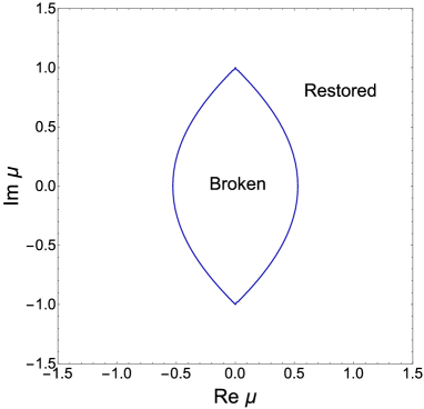
Figure 1: Phase diagram of the random matrix partition function in the complex $\mu$ plane in units where the chiral condensate is equal to 1.

An alternative expression for the fermionic partition function can be obtained by means of the superbosonization technique. The result can be expressed as (see Appendix A)

$${Z^{\nu}(m,\mu)=\frac{(n+1)!e^{n\Sigma^{2}\mu^{2}}}{(n+1-\nu)!}\int_{-\pi}^{\pi}d\beta\int_{-1}^{1}xdxe^{-i\beta(2n+\nu)}x^{\nu}I_{\nu}(2me^{i\beta}x)J_{0}(2\mu e^{i\beta}\sqrt{1-x^{2}})e^{e^{2i\beta}x^{2}/n\Sigma^{2}}.\hskip 56.9055pt}$$

The integrals over $x$ and $\beta$ can be performed analytically resulting in a finite sum that can easily be evaluated numerically.

4.2 The Bosonic Partition Function

After averaging over the chiral random matrix ensemble, the one-flavor bosonic partition function for $\nu=0$ and imaginary chemical potential is given by sener1

$${Z(m,i\mu_{i})=e^{\bar{n}\Sigma^{2}\mu_{i}^{2}}\int d\phi^{*}_{1}d\phi_{1}d\phi^{*}_{2}d\phi_{2}\exp\left[i\left(\begin{array}[]{c}\phi_{1}^{*}\\ \phi_{2}^{*}\end{array}\right)\left(\begin{array}[]{cc}im&\mu_{i}\\ \mu_{i}&im\end{array}\right)\left(\begin{array}[]{c}\phi_{1}\\ \phi_{2}\end{array}\right)-\frac{\phi_{1}^{*}\cdot\phi_{1}\phi_{2}^{*}\cdot\phi_{2}}{\bar{n}\Sigma^{2}}\right],\hskip 28.45274pt}$$ (66)

where the normalization factor $\exp{\bar{n}\Sigma^{2}\mu^{2}}$ is chosen to give a $\mu$-independent partition function in the chiral limit below the critical point. We distinguish $\bar{n}$ appearing in the probability distribution and the number of components $n$ of the vector $\phi_{1}$. Instead of using a Hubbard-Stratonovitch transformation to linearize the quartic term, we use the bosonic part of the superbosonization transformation to evaluate the integral. The starting point is to insert the $\delta$ -function

$$\delta(\Phi-S)$$ (67)

in the partition function with $S$ a positive definite Hermitian matrix and

$$\Phi=\left(\begin{array}[]{cc}\phi_{1}^{*}\cdot\phi_{1}&\phi_{1}^{*}\cdot\phi_{2}\\ \phi_{2}^{*}\cdot\phi_{1}&\phi_{2}^{*}\cdot\phi_{2}\end{array}\right).$$ (70)

The partition function can then be rewritten as

$$Z(m,i\mu_{i})=e^{\bar{n}\Sigma^{2}\mu_{i}^{2}}\int dSd\Phi\delta(S-\Phi)e^{-m{\rm Tr}\Phi+i\mu_{i}{\rm Tr}\sigma_{1}\Phi-S_{11}S_{22}/\bar{n}\Sigma^{2}},$$ (71)

where the integral is over Hermitian matrices $S$. The $\delta$-function can be expressed as Fyodorov

$$\delta(S-\Phi)=\int dFe^{i{\rm Tr}F(S-\Phi-i\epsilon)}$$ (72)

resulting in the partition function

$$Z(m,i\mu_{i})=e^{\bar{n}\Sigma^{2}\mu_{i}^{2}}\int dSdd\Phi dFe^{iFS}e^{-m{\rm Tr}\Phi+i\mu_{i}{\rm Tr}\sigma_{1}\Phi-i{\rm Tr}F\Phi-S_{11}S_{22}/\bar{n}\Sigma^{2}}.$$ (73)

The integral over $\Phi$ evaluates to

$$Z(m,i\mu_{i})=e^{n\mu_{i}^{2}}\int dSdFe^{i{\rm Tr}FS}\frac{1}{\det^{n}[F-im-\sigma_{1}\mu_{i}]}e^{-S_{11}S_{22}/n\Sigma^{2}}.$$ (74)

The integral over $F$ is an Ingham-Siegel integral ingham ; siegel ; Fyodorov ; split-fact which is known analytically,

$$\int dF{\det}^{-n}(F-i\epsilon)e^{i{\rm Tr}SF}=\theta(S){\det}^{n-2}Se^{-\epsilon{\rm Tr}S},$$ (75)

where $\theta(S)$ indicates that $S$ is positive definite. We thus find

$$Z(m,\mu_{i})=e^{\bar{n}\Sigma^{2}\mu_{i}^{2}}\int_{S>0}dS{\det}^{n-2}Se^{-m(S_{11}+S_{22})+i\mu_{i}(s_{12}+s_{21})-S_{11}S_{22}/\bar{n}\Sigma^{2}}.$$ (76)

For $\nu\neq 0$, we choose $\phi_{1}$ to be of length $n+\nu$ and $\phi_{2}$ of length $n$. When comparing different topological sectors moshe , we will put $\bar{n}=n+\nu/2$ and keep $\bar{n}$ fixed so that the number of eigenvalues of the Dirac matrix is the same for different $\nu$. In Eq. (74) this results in an extra factor $1/(F_{11}-iz)^{\nu}$,

$$Z^{\nu}(m,i\mu_{i})=e^{\bar{n}\Sigma^{2}\mu_{i}^{2}}\int dSe^{i{\rm Tr}FS}\frac{1}{\det^{n}[F-im-\sigma_{1}\mu_{i}](F_{11}-im)^{\nu}}e^{-S_{11}S_{22}/\bar{n}\Sigma^{2}},$$ (77)

and after shifting the diagonal matrix elements of $F$ by $im$, we need to evaluate the integral

$$\int dF{\det}^{-n}(F-i\epsilon)(F_{11}-i\epsilon)^{-\nu}e^{i{\rm Tr}SF}.$$ (78)

To calculate this integral we rewrite the determinant to obtain

$$\int dF{(F_{22}-i\epsilon-F_{21}F_{12}/(F_{11}-i\epsilon}))^{-n}(F_{11}-i\epsilon)^{-\nu-n}e^{i{\rm Tr}SF}.$$ (79)

The integral over $F_{22}$ can be performed by a contour integration resulting in

$$\frac{2\pi i^{n}}{(n-1)!}S_{22}^{n-1}\theta(S_{22})\int dFs(F_{11}-i\epsilon)^{-\nu-n}e^{i{\rm Tr}S_{22}\frac{F_{21}F_{12}}{F_{11}-i\epsilon}+iS_{11}F_{11}+iS_{12}F_{21}+iS_{21}F_{12}}.$$

The integral over $F_{12}$ and $F_{21}=F_{12}^{*}$ is a Gaussian integral which can be easily evaluated. We find

$$\frac{2\pi i^{n}}{(n-1)!}S_{22}^{n-1}\frac{\pi i}{S_{22}}\theta(S_{22})\int dF(F_{11}-i\epsilon)^{-\nu-n+1}e^{-i{\rm Tr}S_{12}S_{21}F_{11}/S_{22}+iS_{11}F_{11}}.$$ (81)

Also the integral over $F_{11}$ can be performed by a contour integration so that we finally obtain for the integral (78)

$$-\frac{2\pi(-i)^{\nu+1}}{(n-1)!}S_{22}^{n-2}\pi\frac{2\pi}{(n+\nu-2)!}(S_{11}-S_{12}S_{21}/S_{22})^{n+\nu-2}\theta(S_{22})\theta(S_{11}-S_{12}S_{21}/S_{22})$$ (82)

$$= -\frac{4(\pi(-i))^{nu+1}}{(n-1)!(n+\nu-2)!}{\det}^{n-2}S[\det S/S_{22}]^{\nu}\theta(S),$$

where $\theta(S)$ denotes that $S$ is positive definite.

The integration over positive definite matrices $S$ can be performed by using the parameterization

$$S=e^{v}\left(\begin{array}[]{cc}e^{u}\cosh s&ie^{i\phi}\sinh s\\ -ie^{-i\phi}\sinh s&e^{-u}\cosh s\end{array}\right).$$ (85)

The integration measure is given by

$$dS=4e^{4v}\cosh s\sinh s.$$ (86)

This results in the partition function

$$Z^{\nu}(m,i\mu_{i}) = \frac{e^{\bar{n}\Sigma^{2}\mu_{i}^{2}}}{(n-1)!(n+\nu-2)!}\int dvdudsd\phi\cosh s\sinh se^{2nv}\left[\frac{e^{u+v}}{\cosh s}\right]^{\nu}$$ (87)

$$\times e^{-2me^{v}\cosh s\cosh u-2i\mu_{i}e^{v}\sinh s\sin\phi-e^{2v}\cosh^{2}s/\bar{n}\Sigma^{2}}.$$

The integrals over $u$ and $\phi$ can be expressed in terms of Bessel functions

$$Z^{\nu}(m,i\mu_{i}) = \frac{e^{\bar{n}\Sigma^{2}\mu_{i}^{2}}}{(n-1)!(n+\nu-2)!}\int dvds\frac{\cosh s\sinh s}{\cosh^{\nu}s}e^{(2n+\nu)v}K_{\nu}(2me^{v}\cosh s)J_{0}(2\mu_{i}e^{v}\sinh s)$$ (88)

$$\times e^{-e^{2v}\cosh^{2}s/\bar{n}\Sigma^{2}}.$$

After shifting the $v$-integration by $\log\cosh s$ and choosing $x=\exp v$ as a new integration variable we obtain

$${Z^{\nu}(m,i\mu_{i})=\frac{e^{\bar{n}\Sigma^{2}\mu_{i}^{2}}}{(n-1)!(n+\nu-2)!}\int dxds\frac{\cosh s\sinh s}{\cosh^{2n+2\nu}s}x^{2n+\nu-1}K_{\nu}(2mx)J_{0}(2\mu_{i}x\tanh s)e^{-x^{2}/\bar{n}\Sigma^{2}}.\hskip 56.9055pt}$$

The integral over $y$ can be evaluated as a Bessel function resulting in the expression

$${Z^{\nu}(m,i\mu_{i})=\frac{1}{2}e^{\bar{n}\Sigma^{2}\mu_{i}^{2}}\frac{\mu^{1-n-\nu}\bar{n}^{(n+1)/2}}{(n-1)!}\int_{0}^{\infty}dxx^{n}J_{n+\nu-1}(2\mu_{i}x\sqrt{\bar{n}})K_{\nu}(2mx\sqrt{\bar{n}})e^{-x^{2}/\Sigma^{2}},\hskip 56.9055pt}$$ (90)

where we have also rescaled the integration variable by $\sqrt{\bar{n}}$. This form can easily be evaluated numerically also for large values of $n$. However, because of the oscillatory nature of the integrand, it is not amenable to mean field estimates.

Next we derive an expression for the partition function in terms of a positive definite integrand. This result can be obtained if we insert the following representation for the $K_{\nu}$ function

$$K_{\nu}(x)=\frac{1}{2}\frac{x^{\nu}}{2^{\nu}}\int_{0}^{\infty}\frac{ds}{s^{\nu+1}}e^{-s-x^{2}/4s}$$ (91)

resulting in

$$Z^{\nu}(m,i\mu_{i}) = \frac{1}{4}e^{\bar{n}\Sigma^{2}\mu_{i}^{2}}\frac{\mu_{i}^{1-n-\nu}\bar{n}^{(n+1)/2}}{(n-1)!}\int_{0}^{\infty}ds\frac{(xm\sqrt{\bar{n}})^{\nu}}{s^{\nu+1}}\int_{0}^{\infty}dxx^{n}J_{n+\nu-1}(2\mu_{i}x\sqrt{\bar{n}})$$ (92)

$$\times e^{-s-m^{2}x^{2}\bar{n}/s-x^{2}/\Sigma^{2}}.$$

The integral over $x$ is known analytically ryzhik

$$\int_{0}^{\infty}dxx^{n+\nu}J_{n+\nu-1}(\beta x)e^{-\alpha x^{2}}=\frac{\beta^{n+\nu-1}}{(2\alpha)^{n+\nu}}e^{-\beta^{2}/4\alpha}.$$ (93)

After changing the integration variable be $s\to s\bar{n}m^{2}$ we find

$$Z^{\nu}(m,i\mu_{i}) = \frac{{\bar{n}}^{n}e^{\bar{n}\Sigma^{2}\mu_{i}^{2}}}{8(n-1)!}m^{-\nu}\int_{0}^{\infty}\frac{ds}{s^{\nu+1}}e^{-s\bar{n}m^{2}}\frac{1}{(1/s+1/\Sigma^{2})^{n+\nu}}e^{-\bar{n}\mu^{2}_{i}/(1/s+1/\Sigma^{2})}$$ (94)

$$= \frac{{\bar{n}}e^{n\Sigma^{2}\mu_{i}^{2}}}{8}m^{-\nu}\int_{0}^{\infty}s^{\nu}\frac{ds}{s}e^{-\bar{n}m^{2}/s}\frac{1}{(s+1/\Sigma^{2})^{n+\nu}}e^{-\bar{n}\mu^{2}_{i}/(s+1/\Sigma^{2})},$$

where we also changed $s\to 1/s$ in the last line.

4.3 Limiting Cases

In this subsection, we derive three limiting cases of (94), the microscopic limit, the $\mu_{i}\to 0$ limit, the chiral limit and the large $n$-limit of the bosonic partition function.

In the microscopic limit for the mass, $m\bar{n}={\rm fixed}$ for $\bar{n}\to\infty$ and $n\to\infty$ with $n\to\bar{n}$ at fixed imaginary chemical potential the partition function simplifies to

$$Z^{\nu}(m,i\mu_{i}) = \frac{e^{n\Sigma^{2}\mu_{i}^{2}}}{8(n-1)!}(\bar{n}\Sigma^{2})^{n+\nu}m^{\nu}\int_{0}^{\infty}\frac{ds}{s^{\nu+1}}e^{-s}e^{-\bar{n}^{2}m^{2}\Sigma^{2}/s-\mu^{2}_{i}\bar{n}\Sigma^{2}(1-\bar{n}\Sigma^{2}m^{2}/s)}$$ (95)

$$= \frac{e^{n\Sigma^{2}\mu_{i}^{2}}}{8(n-1)!}(\bar{n}\Sigma^{2})^{n+\nu}m^{\nu}2(\bar{n}m\Sigma\sqrt{1-\mu^{2}_{i}\Sigma^{2}})^{-\nu}e^{-\mu^{2}_{i}\bar{n}\Sigma^{2}}K_{\nu}(2\bar{n}m\Sigma\sqrt{1-\mu^{2}_{i}\Sigma^{2}})$$

$$= \frac{e^{n\Sigma^{2}\mu_{i}^{2}}}{8(n-1)!}\frac{\bar{n}^{n}\Sigma^{2n+\nu}}{(1-\mu^{2}_{i}\Sigma^{2})^{\nu/2}}e^{-\mu^{2}n\Sigma^{2}}K_{\nu}(2\bar{n}m\Sigma\sqrt{1-\mu^{2}_{i}\Sigma^{2}}),$$

which is consistent with the result obtained in sener1 .

For $\mu_{i}=0$ the partition function (88) can be written as

$$Z^{\nu}(m,i\mu_{i}=0)=\int_{0}^{\infty}dxdsx^{2n+\nu-1}\cosh s\sinh sK_{0}(2mx\cosh s)e^{-x^{2}\cosh^{2}s/\bar{n}\Sigma^{2}}.$$ (96)

After rescaling $x$ by $\cosh s$ , the $s$ integral gives an overall constant so that the partition function simplifies to

$$Z^{\nu}(m,i\mu_{i}=0)=\int_{0}^{\infty}dxx^{2n+\nu-1}K_{\nu}(2mx)e^{-x^{2}/\bar{n}\Sigma^{2}}.$$ (97)

This is indeed the Cauchy transform of a Laguerre polynomial ake-fyo , which is the correct finite $n$ result for the chiral random matrix partition function.

For $m\to 0$ we have that

$$K_{\nu}(2mx\sqrt{\bar{n}}) \sim \frac{1}{2}(mx\sqrt{n}b)^{-\nu}\qquad{\rm for}\quad\nu\neq 0,$$

$$K_{0}(2mx\sqrt{\bar{n}}) \sim -\log m\qquad{\rm for}\quad\nu=0.$$ (98)

For $\nu=0$, the chiral limit can be worked out analytically

$$Z^{\nu=0}(m\to 0,i\mu_{i})=-\frac{1}{2}e^{n\Sigma^{2}\mu_{i}^{2}}\frac{\mu^{1-n}\bar{n}^{(n+1)/2}}{(n-1)!}\log m\int_{0}^{\infty}dxx^{n}J_{n-1}(2\mu_{i}x\sqrt{\bar{n}})e^{-x^{2}/\Sigma^{2}}.$$ (99)

This integral is known analytically ryzhik resulting in

$$Z^{\nu=0}(m\to 0,i\mu_{i})=-\frac{\bar{n}^{n}2^{2n-2}}{(n-1)!\Sigma^{2n}}\log m.$$ (100)

In the chiral limit, the partition function is dominated by the logarithmic singularity which does not depend on the imaginary chemical potential. Contrary to the fermionic partition function, it is always in a phase with zero “baryon density”.

For large $n$ the partition function can be evaluated by a saddle point approximation. The saddle point equation for the expression in the second line of (94) reads

$$-\frac{m^{2}}{s^{2}}+\frac{1}{1+s}-\frac{\mu^{2}}{(1+s)^{2}}=0.$$ (101)

To leading order in $m$ the solution is given by

$$\bar{s}=\left\{\begin{array}[]{c}\displaystyle\frac{m}{\sqrt{1-\mu^{2}_{i}}},\quad\mu_{i}<1,\\ \displaystyle\mu^{2}_{i}-1,\quad\mu_{i}>1,\end{array}\right.$$ (104)

resulting in the free energy ($\bar{F}=(\log Z)/n$)

$$\bar{F}=\left\{\begin{array}[]{c}\displaystyle 2m{\sqrt{1-\mu^{2}_{i}}},\quad\mu_{i}<1,\\ \displaystyle 1-\mu^{2}_{i}+\log\mu^{2}_{i}+\frac{m^{2}}{\mu^{2}_{i}-1},\quad\mu_{i}>1.\end{array}\right.$$ (107)

The chiral condensate is given by

$$-\frac{1}{2n}\frac{d\log Z}{dm}=\left\{\begin{array}[]{c}\displaystyle{\sqrt{1-\mu^{2}_{i}}},\quad\mu_{i}<1,\\ \displaystyle\frac{m}{\mu^{2}_{i}-1},\quad\mu_{i}>1,\end{array}\right.$$ (110)

and the baryon number density by

$$-\frac{1}{2n}\frac{d\log Z}{d\mu_{i}}=\left\{\begin{array}[]{c}\displaystyle 0,\quad\mu_{i}<1,\\ \displaystyle-\frac{1}{\mu_{i}}+\mu_{i},\quad\mu_{i}>1.\end{array}\right.$$ (113)

The baryon number susceptibility at imaginary chemical potential is defined by

$$\chi_{B}=-\frac{1}{2n}\frac{d^{2}\log Z}{d\mu^{2}_{i}}=\left\{\begin{array}[]{c}\displaystyle 0,\quad\mu_{i}<1,\\ \displaystyle\frac{1}{\mu_{i}^{2}}+1,\quad\mu_{i}>1.\end{array}\right.$$ (116)

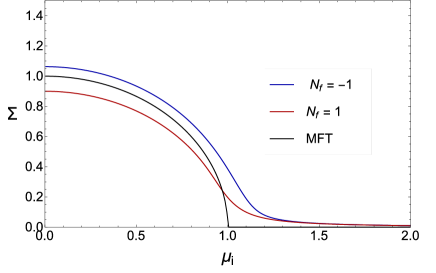
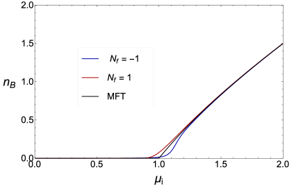
Figure 2: The chiral condensate (left) and the baryon density (right) as a function of the imaginary chemical potential. We show the result for the one-flavor bosonic partition function (blue), the one flavor fermionic partition function (red) and the mean field result (black).

In Fig. 2 we show the chiral condensate (left) and the baryon number (right) as a function of the imaginary chemical potential. The results are for $n=100$, $m=3/100$ in case of the chiral condensate and $n=100$, $m=3/10000$ in case of the baryon number all in units with $\Sigma=1$ in the partition function. Both the results for the fermionic partition function (blue) and the bosonic partition function (red) are close to the mean field result (black) which has been obtained for $n\to\infty$ in the chiral limit.

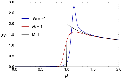
Figure 3: The baryon number susceptibility as a function of the imaginary chemical potential, $\mu_{i}$ for $n=100$ and $m=3/10000$. Results are shown for the fermionic partition function (red), the bosonic partition function (blue), and the mean field limit of these partition functions.

The baryon number susceptibility defined in Eq. (116) is shown in Fig. 3 as a function of the imaginary chemical potential for $n=100$ and $m=3/10000$. Again the bosonic and fermionic susceptibility are close to the mean field result, but the deviation near the critical point is much larger than in case of the baryon number density (see Fig. 2). The convergence of the susceptibility to the thermodynamical limit is non-uniform in $m$.

5 Bosonic Partition Function for Real Chemical Potential

In this section we consider the massless bosonic chiral random matrix partition function for real chemical potential. In this case, the partition function can be expressed in terms of the joint probability distribution of the Ginibre ensemble, which allows us to obtain exact analytical results. We start with a heuristic derivation of the mean field results for the chemical potential dependence of the partition function, and in the second subsection we reduce this partition function to a two-dimensional integral. Everywhere in this section we work in units where $\Sigma=1$ and in the sector of zero topological charge.

5.1 Heuristic Derivation of the Mean Field Result

In units where $\Sigma=1$ and $\nu=0$, the massless bosonic partition function can be expressed as

$$Z_{0/1}(\mu)=e^{-n\mu^{2}}\left\langle\det\frac{1}{D(\mu)}\right\rangle$$ (117)

with $D(\mu)$ given by

$$D(\mu)=\left(\begin{array}[]{cc}0&id+\mu\\ -id^{\dagger}+\mu&0\end{array}\right),$$ (120)

and the normalization factor $\exp(-n\mu^{2})$ has been included to give the correct $\mu$ dependence for small $\mu$. If $\mu$ is inside the domain of eigenvalues, the partition function has to be regularized. This can be done in the same way as for the phase quenched bosonic partition function,

$$Z_{0/1}(\mu)=\left\langle\frac{{\det}^{*}D(\mu)}{\det(D(\mu)D(\mu)^{\dagger}+\epsilon^{2})}\right\rangle,$$ (121)

where the limit $\epsilon\to 0$ has to be taken at the end of the calculation. Contrary to the partition function with a pair of conjugate bosonic quarks at nonzero chemical potential, this partition function, because of the extra fermionic determinant, is finite for $\epsilon\to 0$. At the mean field level we expect that this partition function is given by the ratio of two fermionic partition functions,

$$Z_{0/1}^{\rm MFT}(\mu)=\frac{Z_{N_{f}=1}(\mu)}{Z_{N_{f}=1+1^{*}}(\mu)},$$ (122)

where $Z_{N_{f}=1+1^{*}}(\mu)$ is the phase quenched partition function, or equivalently, the product of the same one flavor partition function and the bosonic phase quenched partition function (see Eq. (52)). The baryon density is thus given by

$$n_{B} = -\frac{1}{2n}\frac{d}{d\mu}\log Z_{0/1}(\mu)$$ (123)

$$\frac{1}{2n}\frac{d}{d\mu}\log Z_{1+1^{*}}(\mu)-\frac{d}{d\mu}\log Z_{1}(\mu).$$

The $\mu$ dependence of both partition functions is well known split-fact ; misha and is given by

$$\frac{1}{2n}\frac{d}{d\mu}\log Z_{1+1^{*}}(\mu) = \theta(1-\mu)4\mu+\theta(\mu-1)(2\mu+\frac{2}{\mu})$$

$$\frac{1}{2n}\frac{d}{d\mu}\log Z_{1}(\mu) = \theta(\mu-\mu_{c})(\mu+\frac{1}{\mu}).$$ (124)

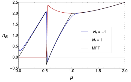
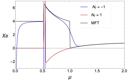
Figure 4: The baryon number density (left) and baryon number susceptibility (right) as a function of the chemical potential, $\mu$ for $n=100$ and $m=0$. Results are give for the fermionic partition function (red), the bosonic partition function (blue), and the mean field limit of the bosonic partition function.

where $\mu_{c}=0.527$. In Fig. 4, the black curve represents the mean field result for the baryon density. In the same figure we have plotted the analytical for finite $n$ (blue curve), which will be derived in the next subsection, and the finite $n$ result for the baryon density of the fermionic partition function (red curve). When $\mu$ is outside the domain of eigenvalues, the fermionic and bosonic results become equal in the thermodynamic limit.

5.2 The Finite $n$ Massless Bosonic Partition Function at Nonzero Chemical Potential

In this section we evaluate the massless bosonic random matrix partition function as a function of the real baryon chemical potential. This partition function can be written as (the equality only holds for even $n$) ipsen-split

$$\left\langle\frac{1}{\det(d+\mu)\det(-d^{\dagger}+\mu)}\right\rangle=\left\langle\frac{1}{\det(d+\mu)\det(d^{\dagger}-\mu)}\right\rangle,$$ (125)

where the matrix elements of the complex $n\times n$ matrix $d$ are distributed according to

$$p(d)=e^{-\bar{n}{\rm Tr}d^{\dagger}d}.$$ (126)

The quenched matrix ensemble with this distribution, known as the Ginibre ensemble, has the joint eigenvalue density

$$P(z_{k})=\Delta(\lambda_{k})\Delta(\lambda^{*}_{k})\prod_{k}e^{-\bar{n}\lambda_{k}^{*}\lambda_{k}},$$ (127)

where $\Delta(\lambda_{k})$ is the Vandermonde determinant. The corresponding monic orthogonal polynomials and their normalization are equal to

$$p_{n}(z)=z^{n},\quad{\rm with}\quad h_{n}=\int dzdz^{*}p_{n}^{*}(z)p_{m}(z)=\delta_{nm}\frac{n!}{\bar{n}^{n+1}}.$$ (128)

The partition function of the Ginibre ensemble, defined as the integral over the probability distribution, can be obtained by expressing the Vandermonde determinants in terms of these orthogonal polynomials. Performing the integrals by means of orthogonality relations we obtain

$$Z_{n}^{\rm G}=n!\prod_{k=0}^{n-1}h_{k}.$$ (129)

In terms of the eigenvalues of $d$, the bosonic partition function can be written as

$$Z_{0/1}(\mu)=\frac{e^{-n\mu^{2}}}{Z_{n}^{\rm G}}\int\prod_{k}d\lambda_{k}d\lambda_{k}^{*}\frac{e^{-\bar{n}\lambda_{k}^{*}\lambda_{k}}}{(\lambda_{k}+\mu)(\lambda_{k}^{*}+\mu)}|\Delta(\lambda_{k})|^{2}.$$ (130)

To evaluate this partition function we need identity

$$u^{n-1}\frac{\Delta_{k}(\lambda_{i})}{\prod_{k=1}^{n}(\lambda_{k}-u)}=\sum_{k=1}^{n}(-1)^{k+n}\frac{\lambda_{k}^{n-1}}{(\lambda_{k}-u)}{\Delta^{\prime}_{k}(\lambda_{i})},$$ (131)

where

$$\Delta^{\prime}_{p}({z_{k}})=\prod_{k<l,kl\neq p}(z_{k}-z_{l}).$$ (132)

This identity can be proved by including the factors $1/(\lambda_{k}-u)$ in the determinant and expanding it with respect to the last row. Applying this identity to the bosonic determinant results in

$$(-1)^{n-1}\mu^{2n-2}\frac{1}{\prod_{k=1}^{n}(\lambda_{k}-u)(\lambda_{k}^{*}+u)}=\sum_{k,l=1}^{n}(-1)^{k+l}\frac{\lambda_{k}^{n-1}{\lambda_{l}^{*}}^{n-1}}{(\lambda_{k}-\mu)(\lambda_{l}^{*}+\mu)}\frac{\Delta^{\prime}_{k}(\lambda_{i})\Delta^{\prime}_{l}(\lambda_{j}^{*})}{\Delta_{k}(\lambda_{i})\Delta_{l}(\lambda_{j}^{*})}.$$ (133)

We can distinguish two types of terms, those with $k=l$, and those with $k\neq l$. All terms of each type give the same contribution to the bosonic partition function. We thus find

$$Z_{0/1}(\mu) = e^{-n\mu^{2}}\frac{n(-1)^{n-1}}{Z_{n}^{\rm G}\mu^{2n-2}}\int\prod_{k}d\lambda_{k}d\lambda_{k}^{*}e^{-\bar{n}\lambda_{k}\lambda_{k}^{*}}\frac{(\lambda_{1}\lambda_{1}^{*})^{n-1}}{(\lambda_{1}-\mu)(\lambda_{1}^{*}+\mu)}\Delta^{\prime}_{1}(\lambda_{i})\Delta^{\prime}_{1}(\lambda_{j}^{*})$$

$$-e^{-n\mu^{2}}\frac{n(n-1)(-1)^{n-1}}{Z_{n}^{\rm G}u^{2n-2}}\int d\lambda_{k}d\lambda_{k}^{*}e^{-\bar{n}\lambda_{k}\lambda_{k}^{*}}\frac{(\lambda_{1}\lambda_{2}^{*})^{n-1}}{(\lambda_{1}-u)(\lambda_{2}^{*}+u)}\Delta^{\prime}_{1}(\lambda_{i})\Delta^{\prime}_{2}(\lambda_{j}^{*}),$$

where the partition function is normalized with respect to the Ginibre partition function (129). This expression can be rewritten as

$$Z_{0/1}(\mu) = e^{-n\mu^{2}}\frac{n(-1)^{n-1}}{Z_{n}^{\rm G}\mu^{2n-2}}\int d\lambda_{1}d\lambda_{1}^{*}e^{-\bar{n}\lambda_{1}\lambda_{1}^{*}}\frac{(\lambda_{1}\lambda_{1}^{*})^{n-1}}{(\lambda_{1}-u)(\lambda_{1}^{*}+u)}Z_{n-1}^{\rm G}$$ (135)

$$+e^{-n\mu^{2}}\frac{n(n-1)(-1)^{n}}{Z_{n}^{\rm G}\mu^{2n-2}}\int d\lambda_{1}d\lambda_{1}^{*}d\lambda_{2}d\lambda_{2}^{*}e^{-\bar{n}(\lambda_{1}\lambda_{1}^{*}-\lambda_{2}\lambda_{2}^{*})}\frac{(\lambda_{1}\lambda_{2}^{*})^{n-1}}{(\lambda_{1}-\mu)(\lambda_{2}^{*}+\mu)}$$

$$\times\langle\pi_{n-2}(\lambda_{2})\pi_{n-2}(\lambda_{1}^{*})\rangle Z_{n-2}^{\rm G}.$$

where the average of two characteristic polynomials is defined by

$$\langle\pi_{n-2}(u)\pi_{n-2}(v^{*})\rangle=\frac{1}{Z_{n-2}^{G}}\int\prod_{k=1}^{n-2}\frac{d\lambda_{k}d\lambda_{l}^{*}}{\pi}\prod_{k=1}^{n-2}(u-\lambda_{k})(v^{*}-\lambda_{k}^{*})e^{-\bar{n}\lambda_{k}\lambda_{k}^{*}}|\Delta(\lambda_{1},\cdots,\lambda_{n-2})|^{2}.$$

This average can be expressed in terms of the two-point kernel of the Ginibre ensemble Akemann:2002vy

$$\langle\pi_{n-2}(u)\pi_{n-2}(v^{*})\rangle=h_{n-2}\sum_{k=0}^{n-2}\frac{(uv^{*})^{k}}{h_{k}}.$$ (137)

This results in the partition function

$$Z_{0/1}(\mu) = \frac{(-1)^{n-1}e^{-n\mu^{2}}}{h_{n}\mu^{2n-2}}\int d\lambda_{1}d\lambda_{1}^{*}e^{-\bar{n}\lambda_{1}\lambda_{1}^{*}}\frac{(\lambda_{1}\lambda_{1}^{*})^{n-1}}{(\lambda_{1}-\mu)(\lambda_{1}^{*}+\mu)}$$

$$-\frac{(-1)^{n-1}e^{-n\mu^{2}}}{h_{n-1}\mu^{2n-2}}\int d\lambda_{1}d\lambda_{1}^{*}d\lambda_{2}d\lambda_{2}^{*}e^{-\bar{n}\lambda_{1}\lambda_{1}^{*}-\bar{n}\lambda_{2}\lambda_{2}^{*}}\frac{(\lambda_{1}\lambda_{2}^{*})^{n-1}}{(\lambda_{1}-\mu)(\lambda_{2}^{*}+\mu)}\sum_{k=0}^{n-2}\frac{(\lambda_{2}\lambda_{1}^{*})^{k}}{h_{k}}.$$

This derivation is also valid for complex values of $\mu$. The first integral in Eq. (5.2) is logarithmically divergent for purely imaginary $\mu$ and has to be regularized which can be done by including a mass term. The resulting logarithmically divergent part of the partition function is $\mu$ independent, which agrees with the result for the chiral limit of the bosonic partition function at imaginary chemical potential which diverges as $\log m$ for $\nu=0$ (see Eq. (100)).

The integrals can be calculated using polar coordinates and converting the angular integral to a contour integral,

$$Z_{0/1}(\mu) = \frac{(-1)^{n-1}e^{-n\mu^{2}}}{h_{n-1}\mu^{2n-2}\pi}\int d\lambda d\phi e^{-\bar{n}\lambda^{2}}\frac{\lambda^{2n-2}}{(\lambda e^{i\phi}-\mu)(\lambda e^{-i\phi}+\mu)}$$

$$-\frac{(-1)^{n-1}e^{-n\mu^{2}}}{h_{n-1}\mu^{2n-2}\pi^{2}}\sum_{k=0}^{n-2}\frac{(-1)^{k+n}}{h_{k}}\left[\int d\lambda d\phi e^{-\bar{n}\lambda^{2}}\frac{\lambda^{n+k}e^{i\phi(n-1-k)}}{(\lambda e^{i\phi}-\mu)}\right]^{2}$$

$$= \frac{2(-1)^{n-1}e^{-n\mu^{2}}}{h_{n-1}\mu^{2n-2}}\left[-\int_{0}^{|\mu|}d\lambda e^{-\bar{n}\lambda^{2}}\frac{\lambda^{2n-1}}{\mu^{2}+\lambda^{2}}+\int_{|\mu|}^{\infty}d\lambda e^{-\bar{n}\lambda^{2}}\frac{\lambda^{2n-1}}{\mu^{2}+\lambda^{2}}\right]$$

$$-\frac{4(-1)^{n-1}e^{-n\mu^{2}}}{h_{n-1}\mu^{2n-2}}\sum_{k=0}^{n-2}\frac{(-1)^{k+n}}{h_{k}}\left[\int_{|\mu|}^{\infty}d\lambda e^{-\bar{n}\lambda^{2}}\lambda^{2k+1}\mu^{n-2-k}\right]^{2}$$

Note that this partition function is not an analytic function of $\mu$ which was also the case for the bosonic partition function of model (9) kim-bos . Because of large cancellations this form of the partition function is not amenable to a mean field analysis. In Appendix B we derive a form where these cancellations have been taken care of analytically. It is given by (for $\mu>0$)

$$Z_{0/1}(u) = \frac{e^{-n\mu^{2}}}{h_{n-1}}\left[\int_{0}^{\infty}dx\frac{e^{-\bar{n}\mu^{2}(2x+1)}}{x+1}-\int_{0}^{1}dx\frac{e^{-\bar{n}\mu^{2}(2x+1)}}{x+1}\left(\frac{\Gamma(n-1,-\bar{n}\mu^{2}x)}{\Gamma(n-1)}\right)\right.$$ (140)

$$\left.+\int_{0}^{1}dx\frac{e^{-\bar{n}\mu^{2}(x+y)}}{x+1}(-x)^{n}\left(1-\frac{\Gamma(n-1,\bar{n}\mu^{2}}{\Gamma(n-1)}\right)\right].$$

We have checked that this result agrees with a direct evaluation of the partition function for $n=2$ and $n=3$. See Appendix C for the brute force expressions for $n=2$ and $n=3$.

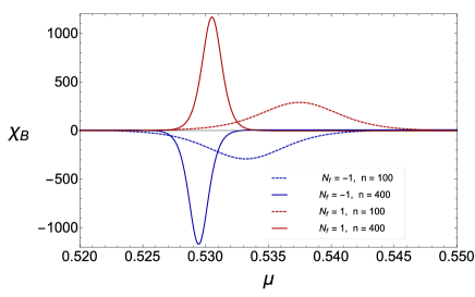
Figure 5: The baryon number susceptibility near the critical point for $\bar{n}=n=100$ (dashed) and $\bar{n}=n=400$ (solid) both for the bosonic 9 (blue) and the fermionic partition function. Up to a minus sign, which could have been absorbed by the definition of the bosonic baryon number susceptibility, the result are similar.

5.3 Large $n$ Limit of the Bosonic Partition Function

In the large $n$ limit, where we take $\bar{n}=n$, the first term of Eq. (140) is given by

$$\frac{1}{h_{n-1}}\frac{1}{4nu^{2}}e^{-4n\mu^{2}}\sim\frac{e^{-n(4\mu^{2}-1)}}{4\mu^{2}\sqrt{2\pi n}},$$ (141)

and the second term by

$$\left\{\begin{array}[]{c}\displaystyle\frac{1}{h_{n-1}\Gamma(n-1)}\frac{e^{-3n\mu^{2}}(-n\mu^{2})^{n-3}}{2n\mu^{2}(1+1/\mu^{2})(1/\mu^{2}-1)}\sim\frac{(-1)^{n}e^{-n(3\mu^{2}-\log\mu^{2}-2)}}{4\pi n^{2}\mu^{2}(1+\mu^{2})(1-\mu^{2})},\qquad{\rm for}\quad\mu<1\\ \displaystyle\frac{1}{h_{n-1}}\frac{e^{-2n\mu^{2}}}{2nu^{2}(1+1/\mu^{2})}\sim\frac{e^{-n(1+2\mu^{2})}}{\sqrt{2\pi n}2n(1+\mu^{2})}\qquad{\rm for}\quad\mu>1\end{array}\right..$$ (144)

The last term factorizes into the product of two integrals. For large $n$ it can be approximated by

$$\left\{\begin{array}[]{c}\displaystyle\frac{\Gamma(n-1)}{h_{n-1}}\frac{(-1)^{n}e^{-n\mu^{2}}}{(n\mu^{2})^{n}(1+1/\mu^{2})}\sim\frac{(-1)^{n}\mu^{2}e^{-n\log\mu^{2}}-n\mu^{2}}{1+\mu^{2}}\qquad{\rm for}\quad u>1\\ \displaystyle\frac{1}{h_{n-1}\Gamma(n-1)}\frac{(-1)^{n}e^{-3n\mu^{2}}(-n\mu^{2})^{n-3}}{2(1-1/\mu^{2})^{2}}\sim\frac{(-1)^{n}e^{-n(3\mu^{2}-\log\mu^{2}-2)}}{4\pi n\mu^{2}(1-\mu^{2})^{2}}\qquad{\rm for}\quad\mu<1\end{array}\right.$$ (147)

This result agrees with the heuristic estimate of section 5.1.

In Fig. 4 we show the baryon number density and the baryon number susceptibility as a function of the chemical potential for $n=100$ and $m=0$. Results are given for fermionic partition function (red), the bosonic partition function (blue) and the mean field limit of the bosonic partition function. The susceptibility diverges at $\mu=\mu_{c}=0.523$ as $\sim n$ in the thermodynamical limit, see Fig. 5. This reflects that the slope

$$\left.\frac{dn_{B}}{d\mu}\right|_{\mu=\mu_{c}}\sim n.$$ (148)

Note that we could have defined the baryon number susceptibility with the opposite sign.

6 Conclusions

We have studied bosonic random matrix partition functions (averages of inverse determinants) and compared them to fermionic random matrix partition functions (averages of a determinants) for the same value of the external parameters. In particular, we consider the dependence of the chiral condensate, the baryon density and the baryon number susceptibility on the (imaginary) chemical potential and the quark mass. For imaginary chemical potential, $\mu_{i}$, and nonzero quark mass, these observables approach the same limit for $n\to\infty$, where the $\mu_{i}$-dependence is given by the mean field result of the effective partition function. In the chiral limit, the bosonic partition function diverges as $\log m$ whereas the fermionic partition function remains finite.

We have seen two cases where the bosonic partition is always in the broken phase while the fermionic partition function undergoes a phase transition to the restored phase. The first case is the phase quenched partition function, where the pion condensate of the bosonic partition function is nonvanishing for all $\mu$ while it is becomes zero for $\mu<m_{\pi}/2$ in case of the fermionic partition function. The second case is the chiral limit of the one flavor partition function as a function of imaginary chemical potential. In this case the fermionic partition function has as phase transition to the restored phase at $\mu_{i}=1$ while the bosonic partition diverges as $\log m$ and is in the same phase for all values of $\mu_{i}$. As a side remark we note that this gives us two more examples where the replica trick is doomed to fail critique .

The spontaneous breaking of noncompact symmetries has also been studied for hyperbolic spin models in one and two dimensions. The conclusion of this work is that a noncompact symmetry is always broken spontaneously, even in one and two dimensions, if the partition function diverges for vanishing symmetry breaking term. Our work supports this conclusion for a different class of models.

Appendix A Derivation of the Fermionic Partition Function Using Superbosonization

Superbosonization was developed as an alternative to the Hubbard-Stratonovitch transformation efetov-original ; martin ; efetov ; akemann-basile ; super-mario in order to be able to deal with non-Gaussian probability distributions. Below we only use the fermion-fermion part of the superbosonization transformation. The fermionic partition function is given by

$$Z^{\nu}(z,\mu)=e^{n\Sigma^{2}\mu^{2}}\int d\chi^{*}_{1}d\chi_{1}d\chi^{*}_{2}d\chi_{2}\exp\left[\left(\begin{array}[]{c}\chi_{1}^{*}\\ \chi_{2}^{*}\end{array}\right)\left(\begin{array}[]{cc}z&\mu\\ \mu&z\end{array}\right)\left(\begin{array}[]{c}\chi_{1}\\ \chi_{2}\end{array}\right)+\frac{1}{n\Sigma^{2}}\chi_{1}^{*}\cdot\chi_{1}\chi_{2}^{*}\cdot\chi_{2}\right],\hskip 14.22636pt$$ (155)

where the vector $\chi_{1}$ is of length $n+\nu$ and the length of the vector $\chi_{2}$ is of length $n$. To linearize the four-fermion term, we use the fermion-fermion part of the superbosonization transformation by inserting the $\delta$-function

$$\delta(G-Y)=\int dFe^{i{\rm Tr}F(G-Y)}$$ (156)

with

$$G=\left(\begin{array}[]{cc}\chi_{1}^{*}\chi_{1}&\chi_{1}^{*}\chi_{2}\\ \chi_{2}^{*}\chi_{1}&\chi_{2}^{*}\chi_{2}\end{array}\right),$$ (159)

and $Y^{\dagger}=Y$. After integration of the $\chi$-variables, this results in the partition function,

$${Z^{\nu}(z,\mu)=e^{n\Sigma^{2}\mu^{2}}\int dYdFF_{11}^{\nu}{\det}^{n}F\exp\left[z(Y_{11}+Y_{22})+\mu(Y_{12}+Y_{21})+\frac{Y_{11}Y_{22}}{n\Sigma^{2}}-i{\rm Tr}FY\right].\hskip 56.9055pt}$$

The integral over $F$ can be evaluated by means of an Itzykson-Zuber integral as

$$[i\partial_{Y_{11}}]^{\nu}\int dF{\det}^{n}Fe^{-i{\rm Tr}FY}$$ (161)

with

$$\int dF{\det}^{n}Fe^{-i{\rm Tr}FY} = \int\prod df_{k}\Delta^{2}(\{f_{k}\})\prod f_{k}^{n}\frac{\det e^{if_{k}y_{l}}}{\Delta(\{f_{k}\})\Delta(\{y_{l}\})}$$ (162)

$$= \frac{\det\delta^{(n+k-1)}(y_{l})}{\Delta(\{y_{l}\})}$$

where $\delta^{(p)}(y)$ is the $p$-th derivative of a $\delta$-function. Acting on a regular test function $F(Y)$, it has the property akemann-basile

$$\int DY\frac{\det\delta^{(n+k-1)}(y_{l})}{\Delta(\{y_{l}\})}F(Y) = \int dY\sum_{\pi}(-1)^{\sigma_{\pi}}\left.\frac{\prod_{k=1}^{p}\partial_{y_{\pi(k)}}^{n+k-1}F(Y)}{\Delta(\{y_{l}\})}\right|_{y_{k}=0}$$ (163)

$$= \int dU\oint\prod_{k}{dy_{k}}{2\pi i}\Delta^{2}(\{y_{l}\})\sum_{\pi}(-1)^{\sigma_{\pi}}\frac{F(Y)}{\Delta(\{y_{l}\})\prod_{k=1}^{p}y_{\pi(k)}^{n+k}}$$

$$= \int dU\oint\prod_{k}\frac{dy_{k}}{2\pi i}\Delta^{2}(\{y_{l}\})\sum_{\pi}(-1)^{\sigma_{\pi}}\frac{F(Y)\prod_{k=1}^{p}y_{\pi(k)}^{p-k}}{\Delta(\{y_{l}\})\prod_{k=1}^{p}y_{k}^{n+p}}$$

$$= \int_{Y\in U(p)}\frac{dY}{(2\pi)^{4}}{\det}^{-n-p}YF(Y),$$

where in the second last equation we have used that the last product is a Vandermonde determinant. Note the measure $dY$ is the product over independent differentials. We thus arrive at the partition function

$$Z^{\nu}(z,\mu) = e^{n\Sigma^{2}\mu^{2}}\int_{Y\in U(2)}\frac{dY}{2\pi^{4}}[[i\partial_{Y_{11}}]^{\nu}{\det}^{-n-2}Y]\exp\left[z(Y_{11}+Y_{22})+\mu(Y_{12}+Y_{21})+\frac{Y_{11}Y_{22}}{n\Sigma^{2}}\right]$$

$$= \frac{(n+\nu+1)!e^{n\Sigma^{2}\mu^{2}}}{(n+1)!}\int_{Y\in U(2)}\frac{dY}{(2\pi)^{4}}\frac{[-iY_{22}]^{\nu}}{{\det}^{n+2+\nu}Y}$$

$$\times\exp\left[z(Y_{11}+Y_{22})+\mu(Y_{12}+Y_{21})+\frac{1}{n\Sigma^{2}}Y_{11}Y_{22}\right].$$

We parameterize $Y$ as

$$Y=e^{i\beta}\left(\begin{array}[]{cc}e^{i\alpha}\cos\theta&e^{i\phi}\sin\theta\\ -e^{-i\phi}\sin\theta&e^{-i\alpha}\cos\theta\end{array}\right),$$ (167)

where $\beta\in[0,2\pi]$, $\phi\in[0,2\pi]$, $\alpha\in[0,\pi]$ and $\theta\in[0,\pi]$. The invariant measure is given by

$$\frac{dY}{(2\pi)^{3}\det^{2}Y}=\frac{\cos\theta\sin\theta d\beta d\alpha d\theta d\phi}{2\pi^{3}}.$$ (168)

This results in the partition function

$$Z^{\nu}(z,\mu) = \frac{(n+\nu+1)!e^{n\Sigma^{2}\mu^{2}}}{2\pi(n+1)!}\int\frac{d\beta d\alpha d\theta d\phi}{(2\pi)^{2}}\cos\theta\sin\theta e^{-2i\beta(n+\nu)}(-i)^{\nu}e^{i\nu(\beta-\alpha)}\cos^{\nu}\theta$$

$$\times e^{2ze^{i\beta}\cos\theta\cos\alpha+2i\mu e^{i\beta}\sin\theta\sin\phi+\frac{1}{n\Sigma^{2}}e^{2i\beta}\cos^{2}\theta}.$$

The integral over $\alpha$ and $\phi$ gives a modified Bessel function so that we finally obtain

$$Z^{\nu}(z,\mu) = \frac{(n+\nu+1)!e^{n\Sigma^{2}\mu^{2}}}{2\pi(n+1)!}\int\frac{d\beta d\theta}{4\pi}\cos\theta\sin\theta e^{-2i\beta n}e^{-i\beta\nu}\cos^{\nu}\theta I_{\nu}(2ze^{i\beta}\cos\theta)$$

$$\times J_{0}(2\mu e^{i\beta}\sin\theta)e^{\frac{1}{n\Sigma^{2}}e^{2i\beta}\cos^{2}\theta}.$$

The normalization will be fixed by the result for $\mu=0$.

$$Z^{\nu}(z,\mu=0) = \frac{(n+\nu+1)!}{(n+1)!}\int d\beta d\theta\cos\theta\sin\theta e^{-2i\beta n}e^{-i\beta\nu}\cos^{\nu}\theta I_{\nu}(2ze^{i\beta}\cos\theta)e^{\frac{1}{n\Sigma^{2}}e^{2i\beta}\cos^{2}\theta}$$ (171)

$$= \frac{(n+\nu+1)!}{(n+1)!}\int d\beta dxxe^{-2i\beta n}e^{-i\beta\nu}x^{\nu}I_{\nu}(2ze^{i\beta}x)e^{\frac{1}{n\Sigma^{2}}e^{2i\beta}x^{2}}$$

$$= \frac{(n+\nu+1)!}{(n+1)!}\int_{0}^{1}dxx\sum_{k+l=n}(zx)^{2k+\nu}x^{\nu}(\frac{1}{n\Sigma^{2}}x^{2})^{l}\frac{1}{k!(k+\nu)!l!}$$

$$= \frac{1}{2}\frac{(n+\nu)!}{(n+1)!}\sum_{k=0}^{n}(z)^{2k+\nu}({n\Sigma^{2}})^{k-n}\frac{1}{k!(k+\nu)!(n-k)!}.$$

The sum is exactly the expression for a Laguerre polynomial so that

$$Z(z,\mu=0) = \frac{z^{\nu}}{(n+1)!\Sigma^{2n}}L_{n}^{\nu}(-z^{2}n\Sigma^{2}).$$ (172)

In the microscopic limit this reduces to

$$Z(z,\mu=0) = \frac{1}{(n+1)!\Sigma^{2n+\nu}}I_{\nu}(2zn\Sigma).$$ (173)

To get the correct $\nu$ dependence we have to include an additional factor of $\Sigma^{\nu}$ in the partition function which was already observed in lehner .

Appendix B Massless one Flavor Bosonic Partition Function

The goal of this appendix to derive a form of the massless bosonic one flavor partition function where the cancellation of the leading order terms has been take care of analytically. The starting point is in the expression in (LABEL:z-bos-1)

$$Z_{n}^{N_{f}=-1}(\mu) = \frac{(-1)^{n-1}}{h_{n-1}}\left[-\int_{0}^{1}dxe^{-\bar{n}\mu^{2}x}\frac{x^{n-1}}{x+1}+\int_{1}^{\infty}dxe^{-\bar{n}\mu^{2}x}\frac{x^{n-1}}{x+1}\right]$$

$$-\frac{(-1)^{n-1}}{h_{n-1}}\sum_{k=0}^{n-2}\frac{(-1)^{k+n}}{h_{k}}\left[\mu^{k+1}\int_{1}^{\infty}dxe^{-\bar{n}\mu^{2}x}x^{k}\right]^{2}.$$

The sum on the second line of this equation can be written as

$$\sum_{k=0}^{n-2}\frac{(-1)^{k}}{h_{k}}\left[\mu^{k+1}\int_{1}^{\infty}dxe^{-\bar{n}\mu^{2}x}x^{k}\right]^{2}$$

$$=\sum_{k=0}^{n-2}\frac{(-1)^{k}}{h_{k}}\mu^{2(+1)}\int_{1}^{\infty}dye^{-\bar{n}\mu^{2}y}y^{k}(\int_{0}^{\infty}dxe^{-\bar{n}\mu^{2}x}x^{k}-\int_{0}^{1}dxe^{-\bar{n}\mu^{2}x}x^{k})$$

$$=\sum_{k=0}^{n-2}\frac{(-1)^{k}}{h_{k}}\mu^{2(k+1)}\int_{1}^{\infty}dye^{-\bar{n}\mu^{2}y}y^{k}\left(\frac{k!}{(\bar{n}\mu^{2})^{k+1}}-\int_{0}^{1}dxe^{-\bar{n}\mu^{2}x}x^{k}\right)$$

$$=\sum_{k=0}^{n-2}\int_{1}^{\infty}dye^{-\bar{n}\mu^{2}y}(-y)^{k}-\frac{\mu^{2(k+1)}}{h_{k}}\int_{0}^{1}dxe^{-\bar{n}\mu^{2}x}x^{k}\int_{1}^{\infty}dye^{-\bar{n}\mu^{2}y}(-y)^{k}$$

$$=\int_{1}^{\infty}dye^{-\bar{n}\mu^{2}y}\frac{1-(-y)^{n-1}}{1+y}-\sum_{k=0}^{n-2}\frac{\mu^{2(k+1)}}{h_{k}}\int_{0}^{1}dxe^{-\bar{n}\mu^{2}x}x^{k}\int_{1}^{\infty}dye^{-\bar{n}\mu^{2}y}(-y)^{k}$$

$$=(-1)^{n}\int_{1}^{\infty}dy\frac{y^{n-1}e^{-\bar{n}\mu^{2}y}}{1+y}+\int_{1}^{\infty}dy\frac{e^{-\bar{n}\mu^{2}y}}{1+y}$$

$$-\sum_{k=0}^{n-2}\frac{\mu^{2(k+1)}}{h_{k}}\int_{0}^{1}dxe^{-\bar{n}\mu^{2}x}x^{k}\int_{1}^{\infty}dye^{-\bar{n}\mu^{2}x}(-y)^{k}$$

$$=(-1)^{n}\int_{1}^{\infty}dy\frac{y^{n-1}e^{-\bar{n}\mu^{2}y}}{1+y}+\int_{1}^{\infty}dy\frac{e^{-\bar{n}\mu^{2}y}}{1+y}$$

$$-\bar{n}\mu^{2}\int_{0}^{1}dx\int_{1}^{\infty}dye^{-\bar{n}\mu^{2}(x+y+xy)}\frac{\Gamma(n-1,-\bar{n}\mu^{2}xy)}{\Gamma(n-1)}$$

Inserting this result in the partition function (LABEL:part1) we find

$$Z(\mu) = \frac{1}{h_{n-1}}\left[-(-1)^{n-1}\int_{0}^{1}dxe^{-\bar{n}\mu^{2}x}\frac{x^{n-1}}{x+1}+\int_{1}^{\infty}dxe^{-\bar{n}\mu^{2}x}\frac{1}{1+x}\right.$$ (176)

$$\left.-\bar{n}\mu^{2}\int_{0}^{1}dx\int_{1}^{\infty}dye^{-\bar{n}\mu^{2}(x+y+xy)}\frac{\Gamma(n-1,-\bar{n}\mu^{2}xy)}{\Gamma(n-1)}\right]$$

$$= {\frac{1}{h_{n-1}}\left[(-1)^{n}\int_{0}^{1}dx\frac{x^{n-1}e^{-\bar{n}\mu^{2}x}}{x+1}+\int_{1}^{\infty}dx\frac{e^{-\bar{n}\mu^{2}x}}{1+x}-\bar{n}\mu^{2}\int_{0}^{1}dx\int_{1}^{\infty}dye^{-\bar{n}\mu^{2}(x+y+xy)}\right.\hskip 56.9055pt}$$

$$\left.-\bar{n}\mu^{2}\int_{0}^{1}dx\int_{1}^{\infty}dye^{-\bar{n}\mu^{2}(x+y+xy)}\left(\frac{\Gamma(n-1,-\bar{n}\mu^{2}xy)}{\Gamma(n-1)}-1\right)\right]$$

$$= \frac{1}{h_{n-1}}\left[-(-1)^{n-1}\int_{0}^{1}dxe^{-\bar{n}\mu^{2}x}\frac{x^{n-1}}{x+1}+\bar{n}\mu^{2}\int_{1}^{\infty}dx\int_{1}^{\infty}dye^{-\bar{n}\mu^{2}(x+y+xy)}\right.$$

$${\left.-\bar{n}\mu^{2}\int_{0}^{1}dx\int_{1}^{\infty}dye^{-\bar{n}\mu^{2}(x+y+xy)}\left(\frac{\Gamma(n-1,-\bar{n}\mu^{2}xy)}{\Gamma(n-1)}-1\right)\right].\hskip 56.9055pt}$$

Next we partial integrate the last term with respect to $y$. This results in

$$Z(\mu) = \frac{1}{h_{n-1}}\left[-(-1)^{n-1}\int_{0}^{1}dxe^{-\bar{n}\mu^{2}x}\frac{x^{n-1}}{x+1}+\bar{n}\mu^{2}\int_{1}^{\infty}dx\int_{1}^{\infty}dye^{-\bar{n}\mu^{2}(x+y+xy)}\right.$$

$$-\int_{0}^{1}dx\frac{e^{-\bar{n}\mu^{2}(2x+1)}}{x+1}\left(\frac{\Gamma(n-1,-\bar{n}\mu^{2}x)}{\Gamma(n-1)}-1\right)$$

$$\left.+\frac{\bar{n}\mu^{2}}{\Gamma(n-1)}\int_{0}^{1}dx\int_{1}^{\infty}dy\frac{e^{-\bar{n}\mu^{2}(x+y)}}{x+1}(-x)^{n-1}(y\bar{n}\mu^{2})^{n-2}\right].$$

When the upper limit of the $y$-integral in the last term is extended to $[0,\infty]$ it is equal to $\Gamma(n-1)$ and cancels the first term. What remains is the $y$-integral over $[0,1]$. We thus find

$$Z(\mu) = \frac{1}{h_{n-1}}\left[\bar{n}\mu^{2}\int_{1}^{\infty}dx\int_{1}^{\infty}dye^{-\bar{n}\mu^{2}(x+y+xy)}-\int_{0}^{1}dx\frac{e^{-\bar{n}\mu^{2}(2x+1)}}{x+1}\left(\frac{\Gamma(n-1,-\bar{n}\mu^{2}x)}{\Gamma(n-1)}-1\right)\right.$$ (178)

$$\left.-\frac{\bar{n}\mu^{2}}{\Gamma(n-1)}\int_{0}^{1}dx\int_{0}^{1}dy\frac{e^{-\bar{n}\mu^{2}(x+y)}}{x+1}(-x)^{n-1}(y\bar{n}\mu^{2})^{n-2}\right].$$

The integrals over $y$ can be performed analytically resulting in

$$Z(u) = \frac{e^{-n\mu^{2}}}{h_{n-1}}\left[\int_{0}^{\infty}dx\frac{e^{-\bar{n}\mu^{2}(2x+1)}}{x+1}-\int_{0}^{1}dx\frac{e^{-\bar{n}\mu^{2}(2x+1)}}{x+1}\left(\frac{\Gamma(n-1,-\bar{n}\mu^{2}x)}{\Gamma(n-1)}\right)\right.$$ (179)

$$\left.-\int_{0}^{1}dx\frac{e^{-\bar{n}\mu^{2}x}}{x+1}(-x)^{n-1}\left(1-\frac{\Gamma(n-1,\bar{n}\mu^{2}}{\Gamma(n-1)}\right)\right].$$

Appendix C Bosonic Partition function for $n=2$ and $n=3$

In this appendix we evaluate the bosonic partition function without relying on the tricks used in section 5.2. Starting from the definition we obtain given by

$$Z_{2}(\mu)Z_{2}^{\rm G} = \frac{1}{\pi^{2}}\int d\lambda_{1}d\lambda_{1}^{*}d\lambda_{2}d\lambda_{2}^{*}|\lambda_{1}-\lambda_{2}|^{2}\prod_{k=1}^{2}\frac{e^{-\bar{n}\lambda_{k}^{*}\lambda_{k}}}{(\lambda_{k}-u)(\lambda_{k}^{*}+\mu)}$$ (180)

$$= \frac{2}{\pi^{2}}\int d\lambda_{1}d\lambda_{1}^{*}(\lambda_{1}^{*}\lambda_{1}-\lambda_{1}\lambda_{2}^{*})\prod_{k=1}^{2}\frac{e^{-\bar{n}\lambda_{k}^{*}\lambda_{k}}}{(\lambda_{k}-\mu)(\lambda_{k}^{*}+\mu)}$$

$$= \frac{2}{\pi^{2}}\int d\lambda_{1}d\lambda_{1}^{*}\frac{\lambda_{1}^{*}\lambda_{1}e^{-\bar{n}\lambda_{1}^{*}\lambda_{1}}}{(\lambda_{1}-\mu)(\lambda_{1}^{*}+\mu)}\int d\lambda_{2}d\lambda_{2}^{*}\frac{e^{-\bar{n}\lambda_{2}^{*}\lambda_{2}}}{(\lambda_{2}-\mu)(\lambda_{2}^{*}+\mu)}$$

$$+2\left(\frac{1}{\pi}\int d\lambda_{1}d\lambda_{1}^{*}\frac{\lambda_{1}e^{-\bar{n}\lambda_{1}^{*}\lambda_{1}}}{(\lambda_{1}-\mu)(\lambda_{1}^{*}+\mu)}\right)^{2}$$

$$= 8\int d\lambda\lambda\frac{\lambda^{2}e^{-\bar{n}\lambda^{2}}}{\lambda^{2}+\mu^{2}}{\rm sign}(\lambda-\mu)\int d\lambda\lambda\frac{e^{-\bar{n}\lambda^{2}}}{\lambda^{2}+\mu^{2}}{\rm sign}(\lambda-\mu)$$

$$+2\left(2\int_{1}^{\infty}d\lambda\frac{\lambda\mu e^{-\bar{n}\lambda^{2}}}{\lambda^{2}+\mu^{2}}+2\int_{0}^{1}d\lambda\frac{\lambda^{3}e^{-\bar{n}\lambda^{2}}}{\mu(\lambda^{2}+\mu^{2})}\right)^{2}.$$

Using the same steps as for $n=2$, for $n=3$ the partition function can be expressed in terms of three integrals

$$Z_{3}(\mu)Z^{G}_{3}=6Z^{a}_{0}(\mu)Z^{a}_{1}(\mu)Z^{a}_{2}(\mu)+6Z^{a}_{0}(\mu)(Z^{b}_{1}(\mu))^{2}-12Z^{c}_{1}(\mu)Z^{b}_{1}(\mu)Z^{b}_{2}(\mu)$$ (181)

where

$$Z_{p}^{a}(\mu) = \mu^{2(p+1)}\int_{0}^{\infty}dx{\rm sign}(x-1)\frac{e^{-\bar{n}\mu^{2}x}x^{p}}{x+1},$$

$$Z_{p}^{b}(\mu) = \mu^{p}\int_{1}^{\infty}dx\frac{e^{-\bar{n}\mu^{2}x}}{x+1}-(-u)^{p}\int_{0}^{1}dx\frac{e^{-\bar{n}\mu^{2}x}x^{p}}{x+1},$$

$$Z_{p}^{c}(\mu) = \mu^{2p+1}\int_{1}^{\infty}dx\frac{e^{-\bar{n}\mu^{2}xx^{p}}}{x+1}+\mu^{2p+1}\int_{0}^{1}dx\frac{e^{-\bar{n}\mu^{2}x}x^{p+1}}{x+1},$$

The $n=2$ partition function can be rewritten in terms of the first two integrals

$$Z_{2}(\mu)Z^{G}_{2}=(2Z^{a}_{0}(\mu)Z^{a}_{1}(\mu)+2(Z^{b}_{1}(\mu))^{2}.$$ (183)

References

- (1) J. J. M. Verbaarschot and T. Wettig, Ann. Rev. Nucl. Part. Sci. 50, 343 (2000) doi:10.1146/annurev.nucl.50.1.343 [hep-ph/0003017].
- (2) J. J. M. Verbaarschot, [arXiv:0910.4134 [hep-th]].
- (3) G. Akemann, [arXiv:1603.06011 [math-ph]].
- (4) F. Farchioni, I. Hip and C. B. Lang, Phys. Lett. B 443, 214 (1998) doi:10.1016/S0370-2693(98)01343-4 [hep-lat/9809016].
- (5) W. Bietenholz, I. Hip, S. Shcheredin and J. Volkholz, Eur. Phys. J. C 72, 1938 (2012) doi:10.1140/epjc/s10052-012-1938-9 [arXiv:1109.2649 [hep-lat]].
- (6) D. Landa-Marban, W. Bietenholz and I. Hip, Int. J. Mod. Phys. C 25, no. 10, 1450051 (2014) doi:10.1142/S012918311450051X [arXiv:1307.0231 [hep-lat]].
- (7) F. Berruto, L. Giusti, C. Hoelbling and C. Rebbi, Phys. Rev. D 65, 094516 (2002) doi:10.1103/PhysRevD.65.094516 [hep-lat/0201010].
- (8) M. Kieburg, J. J. M. Verbaarschot and S. Zafeiropoulos, Phys. Rev. D 90, no. 8, 085013 (2014) doi:10.1103/PhysRevD.90.085013 [arXiv:1405.0433 [hep-lat]].
- (9) P. H. Damgaard, U. M. Heller, R. Narayanan and B. Svetitsky, Phys. Rev. D 71, 114503 (2005) doi:10.1103/PhysRevD.71.114503 [hep-lat/0504012].
- (10) A. D. Jackson, M. K. Sener and J. J. M. Verbaarschot, Nucl. Phys. B 479, 707 (1996) [hep-ph/9602225].
- (11) K. Ziegler, Z. Phys.B - Condensed Matter 43, 275-280(1981)
- (12) M.R. Zirnbauer, private communication.
- (13) T. Spencer and M. R. Zirnbauer, Commun. Math. Phys. 252, 167 (2004) doi:10.1007/s00220-004-1223-3 [math-ph/0410032].
- (14) M. Niedermaier and E. Seiler, Annales Henri Poincare 6, 1025 (2005) doi:10.1007/s00023-005-0233-9 [hep-th/0312293].
- (15) Z. Fodor, K. Holland, J. Kuti, D. Nogradi and C. Schroeder, Phys. Lett. B 681, 353 (2009) doi:10.1016/j.physletb.2009.10.040 [arXiv:0907.4562 [hep-lat]].
- (16) A. Cheng, A. Hasenfratz, G. Petropoulos and D. Schaich, JHEP 1307, 061 (2013) doi:10.1007/JHEP07(2013)061 [arXiv:1301.1355 [hep-lat]].
- (17) Z. Fodor, K. Holland, J. Kuti, D. Nógr/’adi and C. H. Wong, PoS LATTICE 2013, 089 (2014) [arXiv:1402.6029 [hep-lat]].
- (18) A. V. Smilga, Phys. Lett. B 278, 371 (1992). doi:10.1016/0370-2693(92)90209-M
- (19) A. V. Smilga and J. J. M. Verbaarschot, Phys. Rev. D 54, 1087 (1996) doi:10.1103/PhysRevD.54.1087 [hep-ph/9511471].
- (20) J.J.M. Verbaarschot and M.R. Zirnbauer, J. Phys. bf A18, 1093 (1985).
- (21) K. Splittorff and J. J. M. Verbaarschot, Nucl. Phys. B 683, 467 (2004) doi:10.1016/j.nuclphysb.2004.01.031 [hep-th/0310271].
- (22) K. Splittorff and J. J. M. Verbaarschot, Nucl. Phys. B 757, 259 (2006) doi:10.1016/j.nuclphysb.2006.09.011 [hep-th/0605143].
- (23) M. Kellerstien, K. Splittorff and J. Verbaarschot, PoS LATTICE 2015, 059 (2016) [arXiv:1605.03219 [hep-lat]].
- (24) A. D. Jackson and J. J. M. Verbaarschot, Phys. Rev. D 53, 7223 (1996) doi:10.1103/PhysRevD.53.7223 [hep-ph/9509324].
- (25) M. A. Stephanov, Phys. Rev. Lett. 76, 4472 (1996) doi:10.1103/PhysRevLett.76.4472 [hep-lat/9604003].
- (26) J. C. Osborn, Phys. Rev. Lett. 93, 222001 (2004) doi:10.1103/PhysRevLett.93.222001 [hep-th/0403131].
- (27) M. G. Alford, A. Kapustin and F. Wilczek, Phys. Rev. D 59, 054502 (1999) doi:10.1103/PhysRevD.59.054502 [hep-lat/9807039].
- (28) D. Toublan and J. J. M. Verbaarschot, Int. J. Mod. Phys. B 15, 1404 (2001) doi:10.1142/S0217979201005908 [hep-th/0001110].
- (29) D. T. Son and M. A. Stephanov, Phys. Rev. Lett. 86, 592 (2001) doi:10.1103/PhysRevLett.86.592 [hep-ph/0005225].
- (30) G. Akemann, J. C. Osborn, K. Splittorff and J. J. M. Verbaarschot, Nucl. Phys. B 712, 287 (2005) doi:10.1016/j.nuclphysb.2005.01.018 [hep-th/0411030].
- (31) G. Akemann, P. H. Damgaard, J. C. Osborn and K. Splittorff, Nucl. Phys. B 766, 34 (2007) Erratum: [Nucl. Phys. B 800, 406 (2008)] doi:10.1016/j.nuclphysb.2006.12.016, 10.1016/j.nuclphysb.2008.04.012 [hep-th/0609059].
- (32) A. M. Halasz, A. D. Jackson and J. J. M. Verbaarschot, Phys. Rev. D 56, 5140 (1997) doi:10.1103/PhysRevD.56.5140 [hep-lat/9703006].
- (33) C. Lehner, M. Ohtani, J. J. M. Verbaarschot and T. Wettig, Phys. Rev. D 79, 074016 (2009) doi:10.1103/PhysRevD.79.074016 [arXiv:0902.2640 [hep-th]].
- (34) R. A. Janik, M. A. Nowak, G. Papp, J. Wambach and I. Zahed, Phys. Rev. E 55, 4100 (1997) doi:10.1103/PhysRevE.55.4100 [hep-ph/9609491].
- (35) R. A. Janik, M. A. Nowak, G. Papp and I. Zahed, Nucl. Phys. B 501, 603 (1997) doi:10.1016/S0550-3213(97)00418-5 [cond-mat/9612240].
- (36) K. B. Efetov, G. Schwiete, K. Takahashi, Phys. Rev. Lett. 92, 026807 (2004).
- (37) P. Littleman, H.-J. Sommers and M.R, Zirnbauer, Comm. Math. Phys. 283, 243 (2008) [arXiv:0707.2929].
- (38) J.E. Bunder, K.B. Efetov, V.E. Kravtsov, O.M. Yevtushenko and M.R. Zirnbauer, J. Stat. Phys. 129, 809 (2007) [arXiv:0707.2932].
- (39) F. Basile and G. Akemann, JHEP 0712, 043 (2007) doi:10.1088/1126-6708/2007/12/043 [arXiv:0710.0376 [hep-th]].
- (40) V. Kaymak, M. Kieburg and T. Guhr, J. Phys. A 47, 295201 (2014) doi:10.1088/1751-8113/47/29/295201 [arXiv:1402.3458 [math-ph]].
- (41) A.E. Ingham, Proc. Camb. Phil. Soc., 29, 271 (1933).
- (42) C.L. Siegel, Ann. Math. 36, 527 (1935).
- (43) Y. V. Fyodorov, Nucl. Phys. B 621, 643 (2002) [math-ph/0106006].
- (44)
- (45) G. Akemann and Y. V. Fyodorov, Nucl. Phys. B 664, 457 (2003) doi:10.1016/S0550-3213(03)00458-9 [hep-th/0304095].
- (46) I.S. Gradshteyn and I.M. Ryzhik, Table of Integrals, Series, and Products(sixth edition) Academic Press (2000).
- (47) G. Akemann and G. Vernizzi, Nucl. Phys. B 660, 532 (2003) doi:10.1016/S0550-3213(03)00221-9 [hep-th/0212051].
- (48) J. R. Ipsen and K. Splittorff, Phys. Rev. D 86, 014508 (2012) doi:10.1103/PhysRevD.86.014508 [arXiv:1205.3093 [hep-lat]].