A staggered discontinuous Galerkin method for a class of nonlinear elliptic equations

Abstract

In this paper, we present a staggered discontinuous Galerkin (SDG) method for a class of nonlinear elliptic equations in two dimensions. The SDG methods have some distinctive advantages, and have been successfully applied to a wide range of problems including Maxwell equations, acoustic wave equation, elastodynamics and incompressible Navier-Stokes equations. Among many advantages of the SDG methods, one can apply a local post-processing technique to the solution, and obtain superconvergence. We will analyze the stability of the method and derive a priori error estimates. We solve the resulting nonlinear system using the Newton’s method, and the numerical results confirm the theoretical rates of convergence and superconvergence.

1 Introduction

Our aim of this paper is to develop a staggered discontinuous Galerkin (SDG) method for a class of nonlinear elliptic problems arising in, for example, hyperpolarization effects in electrostatic analysis hu2012nonlinear , nonlinear magnetic field problems heise1994analysis , subsonic flow problems feistauer1986finite , and heat conduction.

A detailed introduction to the SDG method is given by chung2009optimal ; chung2006optimal . This class of methods has been successfully applied to a wide range of problems including the Maxwell equation chung2011staggered ; chung2013convergence , acoustic wave equation chung2009optimal , elastic equations chung2015staggered ; lee2016analysis , and incompressible Navier-Stokes equations cheung2015staggered . In these applications, the approximate solutions obtain some nice properties such as energy conservation, low dispersion error and mass conservation. Recently, a connection between the SDG method and the hybridizable discontinuous Galerkin (HDG) method is obtained chung2014staggered ; chung2016staggered . From this perspective, the SDG method acquires some new properties, such as postprocessing and superconvergence properties, from the HDG method cockburn2009superconvergent . We remark that numerical methods based on staggered meshes are important in many applications, see virieux1986p ; tavelli2014staggered .

To begin with, we let $\Omega\subset\mathbf{R}^{2}$ be a bounded and simply connected domain with polygonal boundary $\Gamma$. Also, we let the coefficient $\varrho:\mathbf{R}^{2}\to\mathbf{R}$ be a $L^{\infty}$ function satisfying certain conditions (will be specified). Then, for a given $f\in L^{2}(\Omega)$ we seek $u\in H^{1}_{0}(\Omega)$ such that

$$-\mathrm{div}\left(\varrho(\nabla u(x))\nabla{u(x)}\right)=f(x)\text{ in }\,\Omega,\mbox{ and }u(x)=0\quad\text{on }\,\Gamma,$$ (1)

where $\mathrm{div}$ is the usual divergence operator.

This paper is organized as follows. In Section 2, we will construct the SDG method. In Section 3, we will discuss the implementation of the scheme. In Section 4, we will prove stability estimates and an a priori error estimate of our scheme. Finally, in Section 5, we will numerically show the rate of convergence of our method. Throughout this paper, we use $C$ to denote a generic positive constant, which is independent of the mesh size.

2 The SDG formulation

We introduce new variables, the gradient $\vec{G}:=\nabla u$ and the flux $\vec{U}:=\rho(\vec{G})\vec{G}$. Then the problem (1) can be recasted as the following problem in $\Omega$: Find $(\vec{U},\vec{G},u)$ such that,

$$\begin{gathered}\vec{G}=\nabla u,\quad\vec{U}=\rho(\vec{G})\vec{G},\quad-\mathrm{div}\vec{U}=f\quad\mbox{ in }\Omega,\\ u=0\quad\mbox{ on }\Gamma.\end{gathered}$$ (2)

Next we describe the staggered mesh. Assume $\Omega$ is triangulated by a family of triangles with no hanging nodes, namely, the initial triangulation $\mathcal{T}_{u}$. The triangles in $\mathcal{T}_{u}$ are called the first-type macro element. We denote the set of all edges and all interior edges of $\mathcal{T}_{u}$ by $\mathcal{F}_{u}$ and $\mathcal{F}^{0}_{u}$, respectively. Then we choose an interior point $\nu$ in each first-type macro element. We denote the first-type macro element corresponding to $\nu$ by $\mathcal{S}(\nu)$. By connecting each of these interior points to the three vertices of the triangle, we subdivide each triangle into three subtriangles. We denote the triangulation containing all these subtriangles by $\mathcal{T}$ and assume it is shape-regular. We denote the set of all new edges in this subdivision process by $\mathcal{F}_{p}$. Also, we denote the set of all edges and the set of all interior edges by $\mathcal{F}:=\mathcal{F}_{u}\cup\mathcal{F}_{p}$ and $\mathcal{F}_{0}:=\mathcal{F}^{0}_{u}\cup\mathcal{F}_{p}$, respectively. For each interior edge $e\in\mathcal{F}^{0}_{u}$, there are two triangles $\tau_{1},\tau_{2}\in\mathcal{T}$ such that $e=\tau_{1}\cap\tau_{2}$. We denote the union $\tau_{1}\cup\tau_{2}$ by $\mathcal{R}(e)$. Also, for each boundary edge $e$, we denote the only triangle having $e$ as an edge by $\mathcal{R}(e)$. These elements $\mathcal{R}(e)$ are called the second-type macro element. In Fig. 1, we illustrate two first-type marco elements and a second-type marco element obtained from the subdividing process on two neighboring initial triangles.

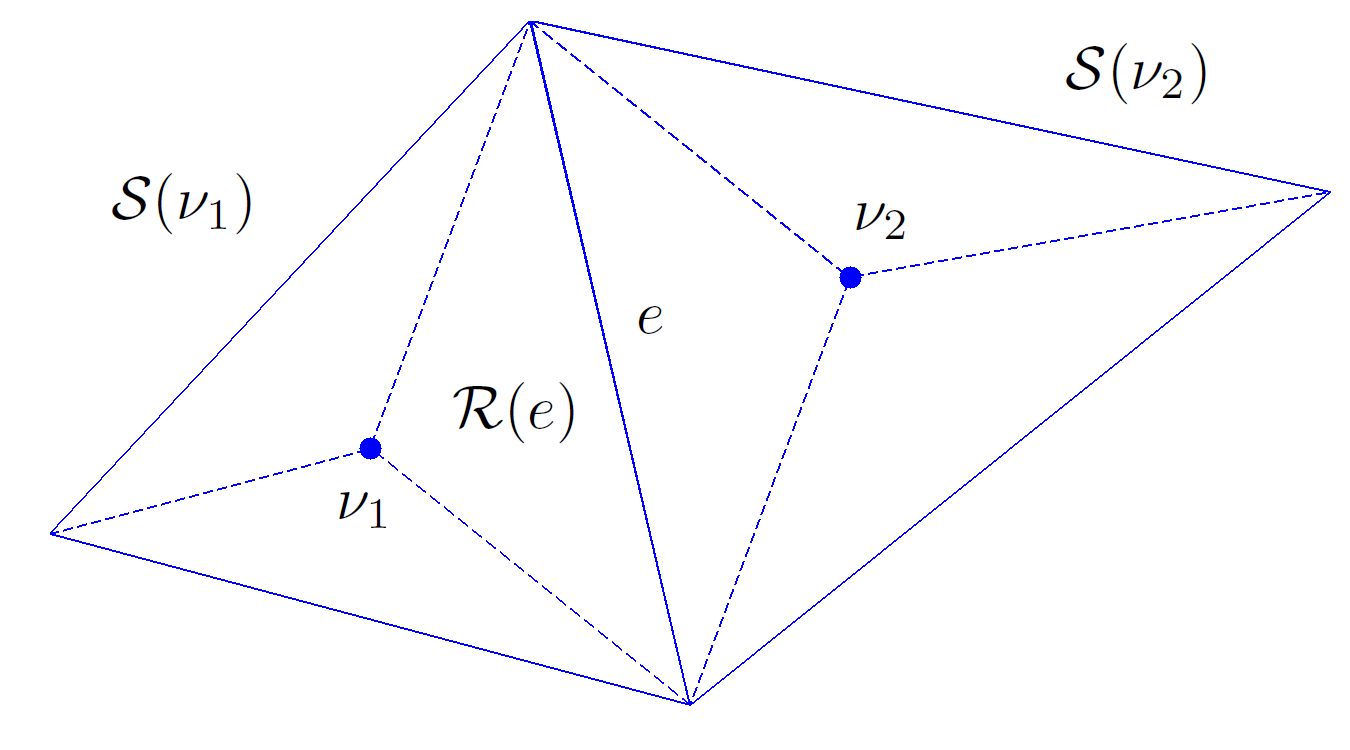
Figure 1: An illustration of the triangulation $\mathcal{T}$.

For a boundary edge $e$, we define $\vec{n}_{e}$ to be the unit normal vector pointing outside $\Omega$. Otherwise, $\vec{n}_{e}$ is one of the two possible unit normal vectors of $e$. When it is clear which edge is being considered, we will simply use $\vec{n}$ instead of $\vec{n}_{e}$.

Next, we describe the finite element spaces we use in our formulation. Let $k\geq 0$ be a non-negative integer. For each triangle $\tau\in\mathcal{T}$, we denote the space of polynomials on $\tau$ with degree at most $k$ by $P^{k}(\tau)$. Then we define the locally $H^{1}(\Omega)$-conforming finite element as

$$\mathcal{U}^{h}:=\{v:v|_{\tau}\in P^{k}(\tau),\forall\tau\in\mathcal{T};v\text{ is continuous across}\;e\in\mathcal{F}^{0}_{u}\;;\;v|_{\partial\Omega}=0\},$$

and the locally $H(\mathrm{div};\Omega)$-conforming finite element space as

$$\begin{gathered}\mathcal{W}^{h}:=\{\mathbf{{V}}:\mathbf{{V}}|_{\tau}\in P^{k}(\tau)^{2},\forall\tau\in\mathcal{T};\text{the normal component }\mathbf{{V}}\cdot\vec{n}_{e}\\ \text{ across}\;e\in\mathcal{F}_{p}\text{ is continuous}\}.\end{gathered}$$

Following chung2009optimal ; chung2006optimal , we consider the following formulation: Find $(\vec{U}_{h},\vec{G}_{h},u_{h})\in\mathcal{W}^{h}\times\mathcal{W}^{h}\times\mathcal{U}^{h}$ such that for any first-type element $\mathcal{S}(\nu)$ and second-type element $\mathcal{R}(e)$, any $(\mathbf{{V}}_{h},\mathbf{{W}}_{h},v_{h})\in\mathcal{W}^{h}\times\mathcal{W}^{h}\times\mathcal{U}^{h}$,

$$\begin{gathered}\int_{\mathcal{S}(\nu)}\vec{G}_{h}\cdot\mathbf{{V}}_{h}\,dx+\int_{\mathcal{S}(\nu)}u_{h}\,\mathrm{div}_{h}\mathbf{{V}}_{h}\,dx-\int_{\partial\mathcal{S}(\nu)}\vec{G}_{h}\left(\mathbf{{V}}_{h}\cdot\vec{n}\right)\,ds=0,\\ \int_{\mathcal{S}(\nu)}\vec{U}_{h}\cdot\mathbf{{W}}_{h}\,dx-\int_{\mathcal{S}(\nu)}\rho(\vec{G}_{h})\vec{G}_{h}\cdot\mathbf{{W}}_{h}\,dx=0,\\ \int_{\mathcal{R}(e)}\vec{U}_{h}\cdot\nabla_{h}v_{h}\,dx-\int_{\partial\mathcal{R}(e)}(\vec{U}_{h}\cdot\vec{n})v_{h}\,ds=\int_{\mathcal{R}(e)}f\cdot v_{h}\,dx,\end{gathered}$$ (3)

where $\nabla_{h}$ and $\mathrm{div}_{h}$ are the elementwise gradient and divergence operators, respectively. Besides, $\vec{n}$ denotes outward normals on $\mathcal{S}(\nu)$ or $\mathcal{R}(e)$ depending on the context.

We define the jump operator $[\cdot]$ as follows. For $e\in\mathcal{F}_{p}$, if $\tau_{1},\tau_{2}\in\mathcal{T}$ such that $e=\tau_{1}\cap\tau_{2}$ and $\vec{n}_{e}$ is pointing from $\tau_{1}$ to $\tau_{2}$, then

$$[v]:=v|_{\tau_{1}}-v|_{\tau_{2}}.$$

For $e\in\mathcal{F}^{0}_{u}$, if $\tau_{1},\tau_{2}\in\mathcal{T}$ such that $e=\tau_{1}\cap\tau_{2}$ and $\vec{n}_{e}$ is pointing from $\tau_{1}$ to $\tau_{2}$, then

$$[\mathbf{{V}}\cdot\vec{n}_{e}]:=\mathbf{{V}}|_{\tau_{1}}\cdot\vec{n}_{e}-\mathbf{{V}}|_{\tau_{2}}\cdot\vec{n}_{e}.$$

We also introduce two bilinear forms,

$$b_{h}(\mathbf{{V}},v):=\int_{\Omega}\textbf{\emph{V}}\cdot\nabla_{\tau}v\;dx-\sum_{e\in\mathcal{F}_{p}}\int_{e}\textbf{\emph{V}}\cdot\textbf{\emph{n}}[v]\;d\sigma,$$

$$b_{h}^{\ast}(v,\mathbf{{V}}):=-\int_{\Omega}v\nabla_{\tau}\cdot\textbf{\emph{V}}\;dx+\sum_{e\in\mathcal{F}_{u}^{0}}\int_{e}v[\textbf{\emph{V}}\cdot\textbf{\emph{n}}]\;d\sigma,$$

for $v\in\mathcal{U}^{h},\textbf{\emph{V}}\in\mathcal{W}^{h}.$ Summing the equations in (3) on $\mathcal{S}(\nu)$ and $\mathcal{R}(e)$, respectively, we can recast (3) into: find $(\vec{U}_{h},\vec{G}_{h},u_{h})\in\mathcal{W}^{h}\times\mathcal{W}^{h}\times\mathcal{U}^{h}$ such that,

$$\int_{\Omega}\vec{G}_{h}\cdot\mathbf{{V}}_{h}\,dx-b^{\ast}_{h}(u_{h},\mathbf{{V}}_{h})=0,\quad\text{ for any }\mathbf{{V}}_{h}\in\mathcal{W}^{h};$$ (4)

$$\int_{\Omega}\vec{U}_{h}\cdot\mathbf{{W}}_{h}\,dx-\int_{\Omega}\rho(\vec{G}_{h})\vec{G}_{h}\cdot\mathbf{{W}}_{h}\,dx=0,\quad\text{ for any }\mathbf{{W}}_{h}\in\mathcal{W}^{h};$$ (5)

$$b_{h}(\vec{U}_{h},v_{h})=\int_{\Omega}fv_{h}\,dx,\quad\text{ for any }v_{h}\in\mathcal{U}^{h}.$$ (6)

This completes the definition of our SDG method.

3 Implementation

In this section we will discuss the implementation detail of our SDG method. First of all we fix a basis $\{\phi_{i}\}_{i=1}^{N_{u}}$ for $\mathcal{U}^{h}$ and $\{\psi_{i}\}_{i=1}^{N_{w}}$ for $\mathcal{W}^{h}$, and write $u_{h}=\sum_{i}(\widehat{u}_{h})_{i}\phi_{i}$, $\vec{G}_{h}=\sum_{i}(\widehat{\vec{G}}_{h})_{i}\psi_{i}$ and $\vec{U}_{h}=\sum_{i}(\widehat{\vec{U}}_{h})_{i}\psi_{i}$, where $\widehat{{u}}_{h}$, $\widehat{\vec{G}}_{h}$ and $\widehat{\vec{U}}_{h}$ are $N_{u}\times 1$, $N_{w}\times 1$ and $N_{w}\times 1$ vectors respectively. Next, we define the mass matrix $M_{h}$ and the matrix $B_{h}$ by $(M_{h})_{ij}:=\int_{\Omega}\psi_{j}\cdot\psi_{i}\,dx,(B_{h})_{ij}:=b_{h}(\psi_{j},\phi_{i}),\mbox{ and}(f_{h})_{i}:=\int fv_{i}\,dx,$ respectively. Then we rewrite (4)–(6) as the following system:

$$M_{h}\widehat{\vec{G}}_{h}-B^{T}_{h}\widehat{u}_{h}=0,$$ (7)

$$M_{h}\widehat{\vec{U}}_{h}=F(\widehat{\vec{G}}_{h}),$$ (8)

$$B_{h}\widehat{\vec{U}}_{h}=\widehat{f}_{h},$$ (9)

where $F(\widehat{\vec{G}}_{h})$ is a $N_{w}\times 1$ vector given by $F(\widehat{\vec{G}}_{h})_{i}:=\left(\rho({\vec{G}}_{h}){\vec{G}}_{h},\psi_{i}\right)_{L^{2}(\Omega)}$. Eliminating $\widehat{\textbf{\emph{U}}}_{h}$ from (7)-(9), we obtain

$$M_{h}\widehat{\vec{G}}_{h}-B^{T}_{h}\widehat{u}_{h} = 0,$$ (10)

$$B_{h}M_{h}^{-1}F(\widehat{\vec{G}}_{h}) = \widehat{f}_{h}.$$ (11)

Here $F$ is not a linear function in general. Hence we use Newton’s method to solve this system. Write $\widehat{\mathbf{x}}_{h}:=(\widehat{\vec{G}}_{h},\widehat{u}_{h})^{T}$ and $H(\widehat{\mathbf{x}}_{h}):=\left(M_{h}\widehat{\vec{G}}_{h}-B_{h}^{T}\widehat{u}_{h},B_{h}M_{h}^{-1}F(\widehat{\vec{G}}_{h})-\widehat{f}_{h}\right)^{T}$. The Jacobian matrix of $H$ is given by

$$\begin{split}J(\widehat{\bf x}_{h}):=\left(\begin{matrix}M_{h}&-B_{h}^{T}\\ B_{h}M_{h}^{-1}F^{\prime}(\widehat{\vec{G}}_{h})&0\end{matrix}\right)\end{split},$$

where $F^{\prime}(\widehat{\vec{G}}_{h})$ is the derivative with respect to $\widehat{\vec{G}}_{h}$, which is given by

$$F^{\prime}(\widehat{\vec{G}}_{h})_{ij}=\left(\rho(\vec{G}_{h})\psi_{j},\psi_{i}\right)+\left((\nabla\rho(\vec{G}_{h})\cdot\psi_{j})\vec{G}_{h},\psi_{i}\right).$$

Given an initial guess $\widehat{\mathbf{x}}_{h}^{0}$, we repeatedly update $\widehat{\mathbf{x}}_{h}^{n}$ by

$$\widehat{{\bf x}}_{h}^{n+1}=\widehat{{\bf x}}_{h}^{n}-[J(\widehat{{\bf x}}_{h}^{n})]^{-1}H({\widehat{\bf x}}_{h}^{n}),$$ (12)

until the successive error $\left\|u_{h}^{n+1}-u_{h}^{n}\right\|$ is less than a given tolerance $\delta$.

4 Stability and convergence of the SDG method

We begin with some results from the SDG method for other problems. We define the discrete $L^{2}$-norm $\|\cdot\|_{X}$ and the discrete $H^{1}$-norm $\|\cdot\|_{Z}$ for any $v\in\mathcal{U}^{h}$ by

$$\|v\|^{2}_{X}:=\int_{\Omega}v^{2}\;dx+\sum_{e\in\mathcal{F}^{0}_{u}}h_{e}\int_{e}v^{2}\;d\sigma\quad\mbox{ and }$$ (13)

$$\|v\|^{2}_{Z}:=\int_{\Omega}|\nabla_{h}v|^{2}\;dx+\sum_{e\in\mathcal{F}_{p}}h^{-1}_{e}\int_{e}[v]^{2}\;d\sigma,$$ (14)

respectively. We also define the discrete discrete $L^{2}$-norm $\|\cdot\|_{X^{\prime}}$ and the discrete $H^{1}$-norm $\|\cdot\|_{Z^{\prime}}$ for any $\mathbf{{V}}\in\mathcal{W}^{h}$ by

$$\|\mathbf{{V}}\|^{2}_{X^{\prime}}=\int_{\Omega}|\mathbf{{V}}|^{2}\;dx+\sum_{e\in\mathcal{F}_{p}}h_{e}\int_{e}(\mathbf{{V}}\cdot\textbf{\emph{n}})^{2}\;d\sigma,$$ (15)

$$\|\mathbf{{V}}\|^{2}_{Z^{\prime}}=\int_{\Omega}(\nabla\cdot\mathbf{{V}})^{2}\;dx+\sum_{e\in\mathcal{F}^{0}_{u}}h^{-1}_{e}\int_{e}[\mathbf{{V}}\cdot\textbf{\emph{n}}]^{2}\;d\sigma.$$ (16)

Then we recall some nice properties of the bilinear forms $b_{h}$ and $b_{h}^{*}$ introduced in previous section. According to Lemma 2.4 of chung2009optimal ,

$$b_{h}(\mathbf{{V}},v)=b_{h}^{\ast}(v,\mathbf{{V}}),\quad\forall(v,\mathbf{{V}})\in\mathcal{U}^{h}\times\mathcal{W}^{h}.$$ (17)

and the following inequality holds:

$$b_{h}(\mathbf{{V}},v)\leq\|v\|_{Z}\|\mathbf{{V}}\|_{X^{\prime}},\quad\forall(v,\mathbf{{V}})\in\mathcal{U}^{h}\times\mathcal{W}^{h}.$$ (18)

From the definition of $\left\|\cdot\right\|_{X}$ and $\left\|\cdot\right\|_{X^{\prime}}$ it is clear that for any $v\in\mathcal{U}^{h}$ and $\mathbf{{V}}\in\mathcal{W}^{h}$,

$$\left\|v\right\|_{L^{2}(\Omega)}\leq\left\|v\right\|_{X},$$ (19)

$$\left\|\mathbf{{V}}\right\|_{L^{2}(\Omega)^{2}}\leq\left\|\mathbf{{V}}\right\|_{X^{\prime}}.$$ (20)

Using the argument in the proof of Lemma 2.1 in Arnold arnold1982interior , we have the following discrete Poincaré inequality.

Lemma 1

For any $v\in\mathcal{U}^{h}$, there is a positive constant $C$ independent of the mesh size $h$ such that

$$\|v\|_{L^{2}(\Omega)}\leq C\|v\|_{Z}.$$ (21)

Moreover, the following inf-sup conditions holds for the bilinear forms $b_{h}$ and $b_{h}^{*}$.

Lemma 2

There is a constant $C$ independent of meshsize $h$ such that

$$\inf_{\mathbf{{V}}\in\mathcal{W}^{h}}\sup_{v\in\mathcal{U}^{h}}\frac{b_{h}^{\ast}(v,\mathbf{{V}})}{\|v\|_{X}\|\mathbf{{V}}\|_{Z^{\prime}}}\geq C,$$

$$\inf_{v\in\mathcal{U}^{h}}\sup_{\mathbf{{V}}\in\mathcal{W}^{h}}\frac{b_{h}(\mathbf{{V}},v)}{\|v\|_{Z}\|\mathbf{{V}}\|_{X^{\prime}}}\geq C.$$

Next, we impose some restrictions on the coefficient $\rho$. We assume $\rho$ is bounded below by a positive number $\rho_{0}$. Moreover, we follow Bustinza and Gatica bustinza2004local to require $\rho(\mathbf{{W}})\mathbf{{W}}$ to be strongly monotone. In order words, there is a positive constant $C$ independent of $\mathbf{{V}},\mathbf{{W}}\in\textbf{\emph{L}}^{2}(\Omega)^{2}$ such that

$$\int_{\Omega}[\rho(\mathbf{{W}})\mathbf{{W}}-\rho(\mathbf{{V}})\mathbf{{V}}]\cdot(\mathbf{{W}}-\mathbf{{V}})\geq C\left\|\mathbf{{W}}-\mathbf{{V}}\right\|_{L^{2}(\Omega)^{2}}^{2};$$ (22)

We also require $\rho(\mathbf{{W}})\mathbf{{W}}$ to be Lipschitz continuous. In order words, there is a positive constant $C$ independent of $\mathbf{{V}},\mathbf{{W}}\in\textbf{\emph{L}}^{2}(\Omega)^{2}$ such that

$$\left\|\rho(\mathbf{{W}})\mathbf{{W}}-\rho(\mathbf{{V}})\mathbf{{V}}\right\|_{L^{2}(\Omega)^{2}}^{2}\leq C\left\|\mathbf{{W}}-\mathbf{{V}}\right\|_{L^{2}(\Omega)^{2}}^{2}.$$ (23)

We will also consider the interpolants $\mathcal{I}:H^{1}(\Omega)\rightarrow\mathcal{U}^{h}$ and $\mathcal{J}:H(\text{div};\Omega)\rightarrow\mathcal{W}^{h}$ discussed in chung2009optimal , which is characterized by

$$b^{\ast}_{h}(\mathcal{I}u-u,\mathbf{{V}}) = 0,\quad\quad\forall u\in H^{1}(\Omega),\mathbf{{V}}\in\mathcal{W}^{h},$$ (24)

$$b_{h}(\mathcal{J}\vec{U}-\vec{U},v) = 0,\quad\quad\forall\vec{U}\in H(\text{div};\Omega),v\in\mathcal{U}^{h}.$$ (25)

It is shown that for any $v\in H^{k+1}(\Omega)$ and $\mathbf{{V}}\in H^{k+1}(\Omega)^{2}$, we have

$$\|v-\mathcal{I}v\|_{L^{2}(\Omega)}\leq Ch^{k+1}\|v\|_{H^{k+1}(\Omega)},$$ (26)

$$\|\mathbf{{V}}-\mathcal{J}\mathbf{{V}}\|_{\textbf{\emph{L}}^{2}(\Omega)}\leq Ch^{k+1}\|\mathbf{{V}}\|_{H^{k+1}(\Omega)^{2}}.$$ (27)

Theorem 4.1

Let $(u,\vec{G},\vec{U})\in H^{k+1}(\Omega)\times H^{k+1}(\Omega)^{2}\times H^{k+1}(\Omega)^{2}$ be the solution of the original problem and $(u_{h},\vec{G}_{h},\vec{U}_{h})$ be the solution of the SDG scheme (4)–(6). Then we have the stability estimate

$$\|u_{h}\|_{L^{2}(\Omega)}+\left\|\vec{U}_{h}\right\|_{L^{2}(\Omega)^{2}}+\left\|\vec{G}_{h}\right\|_{L^{2}(\Omega)^{2}}\leq C\|f\|_{L^{2}(\Omega)},$$ (28)

and the convergence estimates

$$\begin{split}\left\|u-u_{h}\right\|_{L^{2}(\Omega)}+\left\|\vec{U}-\vec{U}_{h}\right\|_{L^{2}(\Omega)^{2}}+\left\|\vec{G}-\vec{G}_{h}\right\|_{L^{2}(\Omega)^{2}}\\ \leq Ch^{k+1}\left(\left\|u\right\|_{H^{k+1}(\Omega)}+\left\|\vec{G}\right\|_{H^{k+1}(\Omega)^{2}}\right).\end{split}$$ (29)

Proof

We start by showing the stability estimate. Taking $\mathbf{{W}}_{h}=\vec{G}_{h}$, $\mathbf{{V}}_{h}=\textbf{\emph{U}}_{h}$, $v_{h}=u_{h}$ in (4)–(6), summing and applying (17), we have

$$\int_{\Omega}\rho(\vec{G}_{h})\vec{G}_{h}\cdot\vec{G}_{h}dx=\int_{\Omega}fu_{h}\,dx.$$ (30)

Applying the Cauchy Schwarz inequality,

$$\|\vec{G}_{h}\|_{L^{2}(\Omega)^{2}}^{2}\leq\rho_{0}^{-1}\|f\|_{L^{2}(\Omega)}\|u_{h}\|_{L^{2}(\Omega)}.$$ (31)

Besides, using Lemma 1 and Lemma 2,

$$\|u_{h}\|_{L^{2}(\Omega)}\leq C\sup_{\mathbf{{V}}\in\mathcal{W}^{h}}\frac{b_{h}(\mathbf{{V}},u_{h})}{\|\mathbf{{V}}\|_{X^{\prime}}}.$$ (32)

Besides, using equations (17) and (4), we have for any $\mathbf{{V}}\in\mathcal{W}^{h}$

$$b_{h}(\mathbf{{V}},u_{h})=\int_{\Omega}\vec{G}_{h}\cdot\mathbf{{V}}\,dx\leq\left\|\vec{G}_{h}\right\|_{L^{2}(\Omega)^{2}}\left\|\mathbf{{V}}\right\|_{L^{2}(\Omega)^{2}}.$$ (33)

Combining (32) and (33) and applying (20),

$$\|u_{h}\|_{L^{2}(\Omega)} \leq C\|\vec{G}_{h}\|_{L^{2}(\Omega)}.$$ (34)

Combining this with (31),

$$\|\vec{G}_{h}\|_{L^{2}(\Omega)^{2}} \leq C\|f\|_{L^{2}(\Omega)},$$ (35)

and the stability estimate (28) follows from the Lipschitz continuity (23).

Next, we show the convergence of $\vec{G}$. Note that (4) and (6) still holds if we replace $\vec{G}_{h}$ by $\vec{G}$, $\vec{U}_{h}$ by $\vec{U}$ and $u_{h}$ by $u$. Therefore,

$$\int_{\Omega}(\vec{G}-\vec{G}_{h})\cdot\mathbf{{V}}\,dx-b^{\ast}_{h}(u-u_{h},\mathbf{{V}}) =0\quad\forall\mathbf{{V}}\in\mathcal{W}^{h},$$ (36)

$$b_{h}(\vec{U}-\vec{U}_{h},v) =0\quad\forall v\in\mathcal{U}^{h}.$$ (37)

Using the properties of $\mathcal{I}$ and $\mathcal{J}$,

$$\int_{\Omega}(\vec{G}-\vec{G}_{h})\cdot\mathbf{{V}}\,dx-b^{\ast}_{h}(\mathcal{I}u-u_{h},\mathbf{{V}}) = 0\quad\forall\mathbf{{V}}\in\mathcal{W}^{h},$$ (38)

$$b_{h}(\mathcal{J}\vec{U}-\vec{U}_{h},v) = 0\quad\forall v\in\mathcal{U}^{h}.$$ (39)

In particular for $v=\mathcal{I}u-u_{h}$ and $\mathbf{{V}}=\mathcal{J}\vec{U}-\vec{U}_{h},$ adding these two equations gives

$$\int_{\Omega}(\vec{G}-\vec{G}_{h})\cdot(\mathcal{J}\vec{U}-\vec{U}_{h})\,dx=0.$$ (40)

On the other hand, from the strong monotonicity (22),

$$\left\|\mathcal{J}\vec{G}-\vec{G}_{h}\right\|^{2}_{L^{2}(\Omega)^{2}}\leq\int_{\Omega}(\mathcal{J}\vec{G}-\vec{G}_{h})\cdot(\mathcal{J}\vec{U}-\vec{U}_{h})\,dx.$$ (41)

Applying equation (40),

$$\begin{split}\left\|\mathcal{J}\vec{G}-\vec{G}_{h}\right\|^{2}_{L^{2}(\Omega)^{2}}&\leq\int_{\Omega}(\mathcal{J}\vec{G}-G)\cdot(\mathcal{J}\vec{U}-\vec{U}_{h})\,dx\\ &\leq C\left\|\mathcal{J}\vec{G}-\vec{G}\right\|_{L^{2}(\Omega)^{2}}\left\|\mathcal{J}\vec{U}-\vec{U}_{h}\right\|_{L^{2}(\Omega)^{2}}.\end{split}$$ (42)

Applying the Lipschitz continuity (23),

$$\left\|\mathcal{J}\vec{G}-\vec{G}_{h}\right\|_{L^{2}(\Omega)^{2}} \leq C\left\|\mathcal{J}\vec{G}-\vec{G}\right\|_{L^{2}(\Omega)^{2}}.$$ (43)

Hence applying (27),

$$\begin{split}\left\|\vec{G}-\vec{G}_{h}\right\|_{L^{2}(\Omega)^{2}}&\leq\left\|\vec{G}-\mathcal{J}\vec{G}\right\|_{L^{2}(\Omega)^{2}}+\left\|\mathcal{J}\vec{G}-\vec{G}_{h}\right\|_{L^{2}(\Omega)^{2}}\\ &\leq Ch^{k+1}\left\|\vec{G}\right\|_{H^{k+1}(\Omega)^{2}}.\end{split}$$ (44)

Then we show the convergence of $u$. Using equation (26),

$$\begin{split}\|u-u_{h}\|_{L^{2}(\Omega)}&\leq\|u-\mathcal{I}u\|_{L^{2}(\Omega)}+\|\mathcal{I}u-u_{h}\|_{L^{2}(\Omega)}\\ &\leq Ch^{k+1}\|u\|_{H^{k+1}(\Omega)}+\|\mathcal{I}u-u_{h}\|_{L^{2}(\Omega)}.\end{split}$$ (45)

Using the inf-sup condition in Lemma 2, equation (17), (24), (36) and (20),

$$\begin{split}\|\mathcal{I}u-u_{h}\|_{L^{2}(\Omega)}&\leq C\sup_{\mathbf{{V}}\in\mathcal{W}^{h}}\frac{b_{h}(\mathbf{{V}},\mathcal{I}u-u_{h})}{\|\mathbf{{V}}\|_{X^{\prime}}}=C\sup_{\mathbf{{V}}\in\mathcal{W}^{h}}\frac{b_{h}^{\ast}(\mathcal{I}u-u_{h},\mathbf{{V}})}{\|\mathbf{{V}}\|_{X^{\prime}}}\\ &=C\sup_{\mathbf{{V}}\in\mathcal{W}^{h}}\frac{b_{h}^{\ast}(u-u_{h},\mathbf{{V}})}{\|\mathbf{{V}}\|_{X^{\prime}}}=C\sup_{\mathbf{{V}}\in\mathcal{W}^{h}}\frac{\int_{\Omega}(\vec{G}-\vec{G}_{h})\cdot\mathbf{{V}}\,dx}{\|\mathbf{{V}}\|_{X^{\prime}}}\\ &\leq C\left\|\vec{G}-\vec{G}_{h}\right\|_{L^{2}(\Omega)^{2}},\end{split}$$ (46)

which shows the convergence of $u_{h}$. The convergence of $\vec{U}_{h}$ follows from the Lipschitz continuity (23).

5 Numerical examples

In this section, we present some numerical examples and verify the convergence rate of our SDG method. Moreover, we will obtain a postprocessed solution $u_{h}^{*}$ which converges with higher order than $u_{h}$. We define the postprocessed solution $u_{h}^{*}$ as follows. For each $\tau\in\mathcal{T}$, we take $u_{h}^{*}\in P^{k+1}(\tau)$ determined by

$$\int_{\tau}\nabla u^{*}_{h}\cdot\nabla w\,dx=\int_{\tau}\vec{G}_{h}\cdot\nabla w\,dx,\quad\forall w\in P^{k+1}(\tau)^{0}$$ (47)

$$\int_{\tau}u_{h}^{*}\,dx=\int_{\tau}u_{h}\,dx,$$ (48)

where $P^{k+1}(\tau)^{0}:=\left\{w\in P^{k+1}(\tau):\int_{\tau}w\,dx=0\right\}$. See cockburn2009superconvergent .

For all of our numerical examples, We consider square domain $\Omega=[0,1]^{2}$. We divide this domain into $N\times N$ squares and divide each square into two triangles. We use this as our initial triangulation $\mathcal{T}_{u}$ and further subdivide each triangle taking the interior points as the centroids of the triangles following the discussion in Section 2. We take the mesh size $h:=1/N$. We illustrate the mesh with $h=1/4$ in Fig. 2.

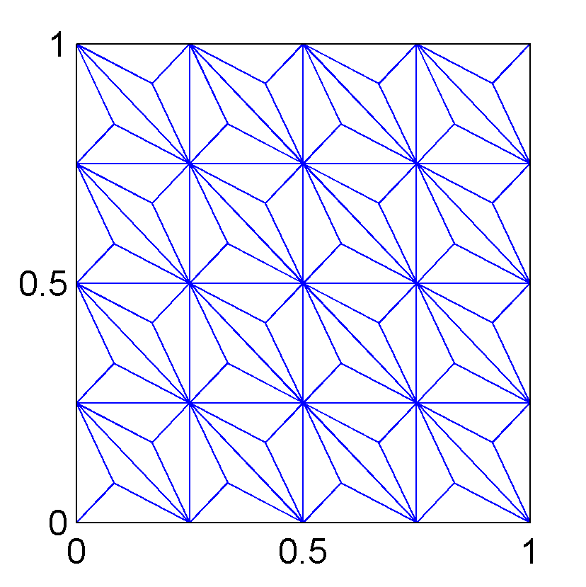
Figure 2: Triangulation on $\Omega=[0,1]^{2}$ with mesh size 1/4.

We consider the following solutions of equation (1).

$$\begin{split}u_{1}(x,y)&=\sin(\pi x)\sin(\pi y),\\ u_{2}(x,y)&=10xy^{2}(1-x)(1-y)-\frac{\mathrm{e}^{x-1}\sin(\pi x)\sin(\pi y)}{2}.\\ \end{split}$$

All these solutions have zero value on the boundary of $\Omega$. We also consider the following six nonlinear coefficients to test the order of convergence.

$$\rho_{1}(\nabla u) :=2+\dfrac{1}{1+|\nabla u|} \rho_{2}(\nabla u) :=1+\exp(-|\nabla u|)$$

$$\rho_{3}(\nabla u) :=1+\exp(-|\nabla u|^{2}) \rho_{4}(\nabla u) :=\dfrac{1}{\sqrt{1+|\nabla u|}}$$

$$\rho_{5}(\nabla u) :=|\nabla u| \rho_{6}(\nabla u) :=|\nabla u|^{2}$$

For each $u_{j}$ and $\rho_{\ell}$, we choose $f$ in (1) and solve for the approximate solution in the spaces of piecewise linear polynomial (i.e. $k=1$), using Newton’s iteration. We terminate the Newton’s iteration when the successive error is less than $\delta=10^{-10}$. Let $u_{j,h}$ be the approximate solution obtained from this Newton’s iteration, and $u_{j,h}^{*}$ be the solution obtained from applying the above postprocessing procedure to $u_{j,h}$. Under different choice of nonlinear coefficients $\rho_{\ell}$, we compute the $L^{2}$ error for $u_{j,h}$ and $u_{j,h}^{*}$, given by $\|u_{j}-u_{j,h}\|_{L^{2}(\Omega)}$ and $\|u_{j}-u^{*}_{j,h}\|_{L^{2}(\Omega)}$, respectively. The results are listed in Table 1 and Table 2. From these results, we see clearly that the scheme gives optimal rate of convergence for the numerical solution and superconvergence for the postprocessed solution.

Coefficient	Mesh size	$||u_{1}-u_{1,h}||_{L^{2}(\Omega)}$	order	$||u_{1}-u_{1,h}^{\ast}||_{L^{2}(\Omega)}$	order	Number of iterations
$\rho_{1}$	$1/4$	3.54e-2	-	2.86e-3	-	4
	$1/8$	9.24e-3	1.94	3.71e-4	2.95	4
	$1/16$	2.34e-3	1.98	4.70e-5	2.98	4
	$1/32$	5.86e-4	2.00	5.91e-6	2.99	4
	$1/64$	1.46e-4	2.00	7.40e-7	3.00	4
$\rho_{2}$	$1/4$	3.50e-2	-	3.00e-3	-	4
	$1/8$	9.23e-3	1.92	3.95e-4	2.82	4
	$1/16$	2.34e-3	1.98	5.07e-5	2.96	4
	$1/32$	5.86e-4	2.00	6.45e-6	2.98	4
	$1/64$	1.46e-4	2.00	8.13e-7	2.99	4
$\rho_{3}$	$1/4$	3.78e-2	-	4.31e-3	-	5
	$1/8$	9.41e-3	2.01	5.46e-4	2.98	5
	$1/16$	2.34e-3	2.01	5.81e-5	3.23	5
	$1/32$	5.86e-4	2.00	7.67e-6	2.92	5
	$1/64$	1.46e-4	2.00	9.84e-7	2.96	5
$\rho_{4}$	$1/4$	3.50e-2	-	3.13e-3	-	4
	$1/8$	9.21e-3	1.93	4.12e-4	2.93	5
	$1/16$	2.34e-3	1.98	5.30e-5	2.96	5
	$1/32$	5.86e-4	2.00	6.74e-6	2.98	5
	$1/64$	1.46e-4	2.00	8.49e-7	2.99	5
$\rho_{5}$	$1/4$	3.60e-2	-	3.32e-3	-	6
	$1/8$	9.29e-3	1.95	5.42e-4	2.62	6
	$1/16$	2.34e-3	1.99	8.34e-5	2.70	7
	$1/32$	5.86e-4	2.00	1.20e-6	2.79	8
	$1/64$	1.47e-4	2.00	1.67e-7	2.85	8
$\rho_{6}$	$1/4$	3.56e-2	-	5.98e-3	-	10
	$1/8$	9.29e-3	1.94	1.50e-3	2.00	10
	$1/16$	2.34e-3	1.99	2.28e-4	2.72	14
	$1/32$	5.86e-4	2.00	3.18e-5	2.84	20
	$1/64$	1.47e-4	2.00	4.29e-6	2.89	27

Table 1: The $L^{2}$ error for $u_{1,h}$ and $u_{1,h}^{*}$ under difference choices of coefficients.

Coefficient	Mesh size	$||u_{2}-u_{2,h}||_{L^{2}(\Omega)}$	order	$||u_{2}-u_{2,h}^{\ast}||_{L^{2}(\Omega)}$	order	Number of iterations
$\rho_{1}$	$1/4$	1.46e-2	-	1.78e-3	-	5
	$1/8$	3.91e-3	1.90	2.40e-4	2.88	5
	$1/16$	9.92e-4	1.98	3.11e-5	2.95	5
	$1/32$	2.49e-4	1.99	3.94e-6	2.98	5
	$1/64$	6.24e-5	2.00	5.00e-7	2.98	5
$\rho_{2}$	$1/4$	1.45e-2	-	1.72e-3	-	5
	$1/8$	3.90e-3	1.90	2.32e-4	2.89	5
	$1/16$	9.91e-4	1.98	3.04e-5	2.93	5
	$1/32$	2.45e-4	1.99	3.82e-6	2.99	5
	$1/64$	6.24e-5	2.00	4.94e-7	2.95	5
$\rho_{3}$	$1/4$	1.40e-2	-	1.90e-3	-	6
	$1/8$	3.94e-3	1.83	2.58e-4	2.88	6
	$1/16$	9.94e-4	1.99	3.22e-5	3.00	6
	$1/32$	2.49e-4	1.99	4.19e-6	2.94	6
	$1/64$	6.24e-5	2.00	5.33e-7	2.97	6
$\rho_{4}$	$1/4$	1.45e-2	-	1.71e-3	-	4
	$1/8$	3.90e-3	1.89	2.31e-4	2.89	4
	$1/16$	9.91e-4	1.98	3.03e-5	2.93	4
	$1/32$	2.49e-4	1.99	3.79e-6	3.00	4
	$1/64$	6.24e-5	2.00	4.89e-7	2.95	4
$\rho_{5}$	$1/4$	1.49e-2	-	3.97e-3	-	7
	$1/8$	3.94e-3	1.92	6.05e-4	2.71	8
	$1/16$	9.99e-4	1.98	9.24e-5	2.71	8
	$1/32$	2.50e-4	2.00	1.32e-5	2.81	10
	$1/64$	6.25e-5	2.00	1.79e-6	2.88	10
$\rho_{6}$	$1/4$	1.54e-2	-	6.54e-3	-	13
	$1/8$	3.91e-3	1.98	1.17e-3	2.49	15
	$1/16$	9.94e-4	1.98	1.96e-4	2.58	18
	$1/32$	2.50e-4	1.99	2.92e-5	2.74	21
	$1/64$	6.24e-5	2.00	3.91e-6	2.90	23

Table 2: The $L^{2}$ error for $u_{2,h}$ and $u_{2,h}^{*}$ under difference choices of coefficients.

References

• (1) D. N. Arnold. An interior penalty finite element method with discontinuous elements. SIAM journal on numerical analysis, 19(4):742–760, 1982.
• (2) R. Bustinza and G. N. Gatica. A local discontinuous Galerkin method for nonlinear diffusion problems with mixed boundary conditions. SIAM Journal on Scientific Computing, 26(1):152–177, 2004.
• (3) S. W. Cheung, E. Chung, H. H. Kim, and Y. Qian. Staggered discontinuous Galerkin methods for the incompressible Navier–Stokes equations. Journal of Computational Physics, 302:251–266, 2015.
• (4) E. Chung, B. Cockburn, and G. Fu. The staggered DG method is the limit of a hybridizable DG method. SIAM Journal on Numerical Analysis, 52(2):915–932, 2014.
• (5) E. Chung, B. Cockburn, and G. Fu. The staggered DG method is the limit of a hybridizable DG method. Part II: the Stokes flow. Journal of Scientific Computing, 66(2):870–887, 2016.
• (6) E. T. Chung, P. Ciarlet, and T. F. Yu. Convergence and superconvergence of staggered discontinuous Galerkin methods for the three-dimensional Maxwell?s equations on Cartesian grids. Journal of Computational Physics, 235:14–31, 2013.
• (7) E. T. Chung and B. Engquist. Optimal discontinuous Galerkin methods for wave propagation. SIAM Journal on Numerical Analysis, 44(5):2131–2158, 2006.
• (8) E. T. Chung and B. Engquist. Optimal discontinuous Galerkin methods for the acoustic wave equation in higher dimensions. SIAM Journal on Numerical Analysis, 47(5):3820–3848, 2009.
• (9) E. T. Chung, C. Y. Lam, and J. Qian. A staggered discontinuous Galerkin method for the simulation of seismic waves with surface topography. Geophysics, 80(4):T119–T135, 2015.
• (10) E. T. Chung and C. S. Lee. A staggered discontinuous Galerkin method for the curl–curl operator. IMA Journal of Numerical Analysis, page drr039, 2011.
• (11) B. Cockburn, J. Guzmán, and H. Wang. Superconvergent discontinuous Galerkin methods for second-order elliptic problems. Mathematics of Computation, 78(265):1–24, 2009.
• (12) M. Feistauer. On the finite element approximation of a cascade flow problem. Numerische Mathematik, 50(6):655–684, 1986.
• (13) B. Heise. Analysis of a fully discrete finite element method for a nonlinear magnetic field problem. SIAM Journal on Numerical Analysis, 31(3):745–759, 1994.
• (14) L. Hu and G.-W. Wei. Nonlinear poisson equation for heterogeneous media. Biophysical journal, 103(4):758–766, 2012.
• (15) J. J. Lee and H. H. Kim. Analysis of a staggered discontinuous Galerkin method for linear elasticity. Journal of Scientific Computing, 66(2):625–649, 2016.
• (16) M. Tavelli and M. Dumbser. A staggered semi-implicit discontinuous Galerkin method for the two dimensional incompressible Navier-Stokes equations. Applied Mathematics and Computation, 248:70–92, 2014.
• (17) J. Virieux. P-SV wave propagation in heterogeneous media: Velocity-stress finite-difference method. Geophysics, 51(4):889–901, 1986.