Gibbsian On-Line Distributed Content Caching Strategy for Cellular Networks

Abstract

In this paper, we develop Gibbs sampling based techniques for learning the optimal placement of contents in a cellular network. We consider the situation where a finite collection of base stations are scattered on the plane, each covering a cell (possibly overlapping with other cells). Mobile users request for downloads from a finite set of contents according to some popularity distribution which may be known or unknown to the base stations. Each base station has a fixed memory space that can store only a strict subset of the contents at a time; hence, if a user requests for a content that is not stored at any of its serving base stations, the content has to be downloaded from the backhaul. Hence, we consider the problem of optimal content placement which minimizes the rate of download from the backhaul, or equivalently maximize the cache hit rate. It is known that, when multiple cells can overlap with one another (e.g., under dense deployment of base stations in small cell networks), it is not optimal to place the most popular contents in each base station. However, the optimal content placement problem is NP-complete. Using ideas of Gibbs sampling, we propose simple sequential content update rules that decide whether to store a content at a base station (if required from the base station) and which content has to be removed from the corresponding cache, based on the knowledge of contents stored in its neighbouring base stations. The update rule is shown to be asymptotically converging to the optimal content placement for all nodes under the knowledge of content popularity. Next, we extend the algorithm to address the situation where content popularities and cell topology are initially unknown, but are estimated as new requests arrive to the base stations; we show that our algorithm working with the running estimates of content popularities and cell topology also converges asymptotically to the optimal content placement. Finally, we demonstrate the improvement in cache hit rate compared to most popular content placement and independent content placement strategies via numerical exploration.

I Introduction

The proliferation of smartphones and tablets equipped with 3G and 4G connectivity and the fast growing demand for downloading multimedia files have resulted in severe overload in the internet backhaul, and it is expected to be worse with the advent of 5G in near future. Recent idea of densifying cellular networks will improve wireless throughput, but this will eventually push the backhaul bandwidth to its limit. In order to alleviate this problem, the idea of caching popular multimedia contents has recently been proposed. Given the fact that the popular contents are requested many times which results in network congestion, one way to reduce the congestion is to cache the popular contents at various intermediate nodes in the network. In case of cellular network, this requires adding physical memory to base stations (BSs): macro, micro, nano and pico. This has several advantages: (i) Caching contents at base stations reduce backhaul load. (ii) Caching reduces delay in fetching the content, thereby reducing the multimedia playback time. (iii) Caching will allow the end user to download a lower quality content in case his channel quality or bad or in case he wants to control his total amount of download.

Under dense placement of base stations, it is often the case that the cells (a cell is defined to be a region around a BS where the user is able to get sufficient downlink data rate from the BS) of different BSs might overlap with each other in an arbitrary manner (see [1]). Hence, if a user is covered by multiple BSs, she has the option to download a content from any one of the serving BSs. This gives rise to the problem of optimal content placement in the caches of cellular BSs (see [2], [3]); the trade-off is that ideally the caching strategy should avoid placing the same content in two BSs whose cells have a significant overlap, while it is not desirable for the non-overlapped region. Optimal content placement under such situation requires global knowledge of base station locations and cell topologies, and solving the optimization problem requires intensive computation. In order to tackle these problems, we develop sequential cache update algorithms motivated by Gibbs sampling, that asymptotically lead to optimal content placement, where each base station updates its contents only when a new content is downloaded from the backhaul to meet a user request, and this update is made solely based on the knowledge of the neighbouring BSs whose cells have nonzero intersection with the cell of the BS under consideration. The results are also extended to the case where the content popularities and cell topology are unknown initially and are learnt over time as new content requests arrive to the base stations. Numerical results demonstrate the improvement in cache hit rate using Gibbs sampling technique for cache update, compared to most popular content placement and independent content placement strategies in the caches.

I-A Related Work

There have been considerable amount of work in the literature dedicated to cellular caching. Benefits and challenges for caching in 5G networks have been described in [6]. The authors of [7] have developed a method to analyze the performance of caches (isolated or networked), and shown that placing the most popular subset of contents in each cache is not optimal in case of interconnected caches. The paper [3] deals with optimal content placement in wireless caches given BS-user association. The authors of [8] have addressed the problem of optimal content placement under user mobility. The authors of [2] have proposed a randomized content placement scheme in cellular BS caches in order to maximize cache hit rate, but their scheme assumes that the contents are placed independently across the caches, which is obviously suboptimal. This work was later extended to the case of heterogeneous networks in [9]. The authors of [10] have again considered independent probabilistic caching in a random heterogeneous network. The paper [11] has addressed the problem of cache miss minimization in a random network setting. The authors of [12] have studied the problem of distributed caching in ultra-dense wireless small cell networks using mean field games; however, this formulation requires us to take base station density to infinity (which may not be true in practice), and it does not provide any guarantee on the optimality of this caching strategy. The paper [13] proposes a pricing based scheme for jointly assigning content requests to cellular BSs and updating the cellular caches; but this paper focuses on certain cost minimization instead of hit rate maximization, and it is optimal only when we can represent the data by very large number of chunks which can be used in employing rateless code. The problem of collaborative but decentralized caching among small base stations for a certain cost minimization has been analyzed in [14], under the assumption that the caches have access to the contents of other caches connected to the same gateway; their formulation involves a certain cost for retrieval of a content from another cache. The authors of [15] address the problem of minimizing energy consumption under multi-cell transmission cooperation for interference reduction and content caching in heterogeneous networks. Since content providers might have to pay cellular network operators for caching their contents, an important question is how to cache contents among multiple base stations to that the content placement charge is minimized; this problem has been addressed by the work reported in [16]. The authors of [17] have considered the problem of collaborative content placement at caches of multiple base stations, but under the assumption that cache sizes at base stations are unlimited. The paper [18] discusses cooperative content caching and delivery policy among multiple base stations. The paper [19] provides a fast but suboptimal solution based on potential game formulation, to the problem of minimizing cache miss rate when multiple base stations have overlapping cells. [19] also provided one simulated annealing-based algorithm (different from our Gibbs sampling approach) that minimizes the cache miss rate.

The paper [20] analyzes a stochastic geometry framework where cache-enabled small base stations are randomly placed on infinite two dimensional plane, and calculated the expressions for the outage probability of a typical user (jointly in terms of SINR and content availability at the cache), as well as the delivery rate. The authors of [21], for a randomly deployed heterogeneous network, derive approximate expressions for the average delivery rate considering inter-tier and intra-tier dependence. The authors of [22] analyze the average delay of users for a random two-tier network under perfect knowledge of content popularity distribution and randomized caching policies. All of these papers consider a stochastic geometry framework for base station locations, and assume limited backhaul. However, in our current paper, we consider known placement of a finite number of base stations, and seek to maximize the cache hit rate over the entire network; thus, our work seeks to reduce the load in the backhaul without imposing a hard constraint on the backhaul capacity. It is worth mentioning that, under this setting, we provide decentralized cache update schemes which are hit-rate optimal for a finite network in a time-average sense.

The authors of [23] and [24] propose learning schemes for unknown time-varying popularity of contents, but their scheme does not have theoretical guarantee of convergence to the optimal content placement across the network when cells of different BSs overlap with each other. The paper [25] establishes that, when popularity is dynamic, any scheme that separates content popularity estimation and cache update (i.e., control) phases is strictly order-wise suboptimal in terms of hit rate. A big data approach has been taken in [26] for estimating content popularities empirically from mobile traffic data collected from a telecom operator. The authors of [27] proposed simulated annealing based caching for a single cache, and also addressed the issue of unknown content popularities by proposing an algorithm that avoids direct popularity estimation.

Contrary to the prior literature, our current paper provides theoretical guarantee of convergence for an optimal distributed cellular cache update scheme that maximizes the time-average cache hit rate over the network involving caches in multiple base stations with overlapping cells; this minimizes the amount of data downloaded from the backhaul. The results also hold when popularities and cell topology are unknown initially and are learnt over time using the information of request arrivals in the base stations.

I-B Organization and Our Contribution

The rest of the paper is organized as follows.

• The system model has been defined in Section II.

• In Section III, we propose an update scheme for the caches based on the knowledge of the contents cached in neighbouring BSs. The update scheme is based on Gibbs sampling techniques, and cache updates are made only when new content requests arrive. The scheme asymptotically converges to a near-optimal content placement in the network, since the scheme is proposed for a finite “inverse temperature” to be defined later. We prove convergence of the proposed scheme. To the best of our knowledge, such a scheme has never been used in the context of caching in cellular network.

• In Section IV, we discuss how to slowly increase the inverse temperature to $\infty$ so that the near-optimal limiting solution in Section III actually converges to the globally optimal solution. We provide rigorous proof for the convergence of this scheme.

• In Section V, we discuss how to adapt the update schemes to the situation when unknown content popularities and cell topology are learnt over time as new content requests arrive to the BSs over time.

• In Section VI, we numerically demonstrate that the proposed Gibbs sampling approach has the potential to significantly improve the cache hit rate in cellular networks.

• Finally, we conclude in Section VII.

II System Model and Notation

II-A Network Model

We consider a finite set $\mathcal{N}:=\{1,2,\cdots,N\}$ of base stations (BSs) on the two-dimensional Euclidean space. The location of the base stations are deterministic and arbitrary; for example, the locations could come from a given realization of a point process over a finite geographical region. The set of points covered by a BS constitute the cell of the corresponding BS. This coverage could be signal to noise ratio (SNR) based coverage where a point is covered by a BS if and only if the SNR at that point from the BS exceeds some threshold. We denote the cell of BS $i$ ($1\leq i\leq N$) by $\mathcal{C}_{i}$. Let us define $\mathcal{C}:=\cup_{i=1}^{N}\mathcal{C}_{i}$. The area of any subset $\mathcal{A}$ of $\mathbb{R}^{2}$ is denoted by $|\mathcal{A}|$. We allow the cells of various BSs to have arbitrary and different finite areas. The cells of two BSs might have a nonzero intersection; any downlink mobile user located at such an intersection is covered by more than one BS. Let us denote by $2^{\mathcal{N}}$ the collection of all subsets of $\mathcal{N}$, and let $s$ denote one such generic subset. Let us denote by $\mathcal{C}(s):=(\cap_{i\in s}\mathcal{C}_{i})\cap(\cup_{i\notin s}\mathcal{C}_{i})^{c}$ the region in $\mathcal{C}$ which is covered only by the BSs from the subset $s$. See Figure 1 for a better understanding of the cell model.

Figure 1: A pictorial description of the base station coverage model. In the diagram, four BSs are shown with numbers $1,2,3,4$. The circles correspond to the cells of the BSs. The region marked as $\{1,2,3\}$ has $s=\{1,2,3\}$; i.e., this region is called $\mathcal{C}(\{1,2,3\})$ and it is covered only by BSs $\{1,2,3\}$ and no other BS. Similar meaning applies to other regions.

II-B Content Request Process

Contents from a set $\mathcal{M}:=\{1,2,\cdots,M\}$ are requested by users located inside $\mathcal{C}$. We assume that each of these contents have the same size, though we will explain at the end of Section III how to easily take care of unequal content sizes in our analysis. Content $i$ ($1\leq i\leq M$) is requested by users according to a homogeneous Poisson point process in space (inside $\mathcal{C}$) and time with intensity $\lambda_{i}$; this is the expected number of requests for content $i$ per second per square meter inside $\mathcal{C}$. Let $\lambda:=\sum_{i=1}^{M}\lambda_{i}$. Note that, $\frac{\lambda_{i}}{\lambda}$ denotes the probability that a content request is for content $i$; in other words, $\frac{\lambda_{i}}{\lambda}$ is the popularity of content $i$. We also assume that $\lambda_{1}\geq\lambda_{2}\geq\cdots\geq\lambda_{M}$.

It is worth mentioning that the cache request process essentially follows the popularly known independent request model (IRM) as described in [28]. In our model, the total request arrival process to the system is a time-homogeneous Poisson process with intensity $\lambda|\mathcal{C}|$. The only difference with IRM is that unlike IRM, the popularity of content $i$ in our model, $\frac{\lambda_{i}}{\lambda}$, can be arbitrary and do not necessarily follow a power law; this makes our request arrival model more general. As an example, this model is valid when users are scattered on the two-dimensional plane according to a homogeneous Poisson point process, and each user is generating content requests according to a time-homogeneous Poisson process, and any new request is for content $i$ with probability $\frac{\lambda_{i}}{\lambda}$.

II-C Content Caching at BSs

We assume that each BS can store $K$ number of contents, where $K<M$. Let $B$ denote a generic configuration of content placement in caches of the network. $B$ is defined as a $M\times N$ matrix with $B_{i,j}=1$ if content $i$ is stored at the cache of BS $j$, and $B_{i,j}=0$ otherwise. Note that, any feasible $B$ must satisfy $\sum_{i=1}^{M}B_{i,j}=K$ for all $j\in\{1,2,\cdots,N\}$; we rule out the possibility of $\sum_{i=1}^{M}B_{i,j}<K$ since that will be a waste of cache memory resources in BSs. Let us denote the set of all feasible configurations by $\mathcal{B}$. Clearly, the cardinality of $\mathcal{B}$ is ${{M}\choose{K}}^{N}$. Apart from $B$, we will also use the symbol $A$ for a generic configuration belonging to set $\mathcal{B}$.

II-D Cache Hit Rate Maximization Problem

We assume that, whenever a new request for a content arrives, it is served by one BS covering that point and having the content in its cache; if a content request is served from the cache, we call the event as a cache hit. In case no covering BS has the content (i.e., no cache hit, or cache miss), the content needs to be downloaded by one of the covering BSs and served to the user (this will be explained later). The requests do not tolerate any delay; i.e., we do not consider the possibility of holding the requests in a queue and serving the content to users in batch once the content becomes available in a BS. Also, we assume infinite bandwidth available for all downlink transmissions; i.e., each content is assumed to be served instantaneously.

Let the random variable $H_{B}$ denote the number of cache hits in the entire network in unit time, under configuration $B$. We define the cache hit rate $h(B)=\mathbf{E}(H_{B})$ where the expectation is over the randomness in the content request arrival process. Clearly,

$$h(B)=\sum_{s\in 2^{\mathcal{N}}}|\mathcal{C}(s)|\sum_{i=1}^{M}\lambda_{i}\mathbf{1}\{\sum_{j\in s}B_{i,j}\geq 1\}.$$ (1)

In this paper, we are interested in finding an optimal configuration which achieves:

$$\sup_{B\in\mathcal{B}}h(B).$$ (2)

Cache hit rate has been considered as the objective function in prior literature; see [11], [2], [7] and [29] for reference. The authors of [29] considered hit rate maximization under coded caching. However, one can consider other objective functions such as latency in content delivery as in [30]; we choose cache hit rate since it is a commonly used objective function. Cache hit rate is a suitable objective function when the requested content needs to be served instantaneously; if the requests are delay-tolerant, then queueing of the requests and contents are allowed and there latency in content delivery would be a more suitable objective function. It is worth mentioning that, in case requests and contents are allowed to be queued at the base station, there is no formal proof that maximizing hit rate will minimize the latency in content delivery, though intuitively one can expect so.

(2) is an optimization problem with $0-1$ integer variables, nonlinear objective function and linear constraints. This class of problems has been shown to be NP-complete (see [31]), and hence, we cannot expect any polynomial time algorithm to solve (2). Hence, in this section, we provide iterative, distributed cache update scheme that asymptotically solves the problem. However, since the algorithm is iterative, we cannot use the optimal configuration over infinite time horizon. Hence, we seek to design a randomized iterative cache update scheme which yields

$$\liminf_{T\rightarrow\infty}\frac{\int_{0}^{T}\mathbf{E}(h(R(\tau)))d\tau}{T}=\sup_{B\in\mathcal{B}}h(B).$$ (3)

where $R(\tau)\in\mathcal{B}$ is the configuration of all caches in the network at time $\tau$. Our iterative scheme is randomized, which renders $R(\tau)$ a random variable; hence, we work with the expectation $\mathbf{E}$.

It is important to note that, by maximizing the cache hit rate, we seek to minimize the download rate from the backhaul; this is necessary because backhaul capacity is limited in practice, and, also, downloading a content from a server via the backhaul link might involve certain cost. However, we do not consider any specific upper limit on the backhaul link capacity. If the backhaul link is blocked due to heavy load or due to finite backhaul capacity, a content request which is not able to find a match in the caches of its covering base stations can either be dropped or kept waiting for service hoping that the backhaul load will be reduced later. If the content request arrival statistics is approximately known to the network operator prior to cache installation at the base stations, the operator can simulate the cache update scheme and estimate the average download rate required for the backhaul under the scheme; this estimate can be used as a design guideline for choosing the backhaul capacity. Hence, for the rest of the paper, we assume sufficient backhaul capacity to deal with cache miss.

III Cache Update via Basic Gibbs Sampling

In this section, we propose an iterative, randomized cache update scheme so that the time-average occupancy of each $B\in\mathcal{B}$ under the scheme follows certain distribution called Gibbs distribution. In Section IV, we explain how tuning a certain parameter of the Gibbs distribution helps us in solving problem (3).

Let us rewrite (1) as $h(B)=\sum_{j=1}^{N}h_{j}(B)$ where

$$h_{j}(B)=\sum_{i=1}^{M}\lambda_{i}\sum_{s\in 2^{\mathcal{N}}}\frac{|\mathcal{C}(s)|B_{i,j}\mathbf{1}\{j\in s\}}{\max\{1,\sum_{k\in s}B_{i,k}\}}.$$ (4)

We call $h_{j}(B)$ to be the cache hit rate seen by BS $j$ under configuration $B$. This will be the true cache hit rate seen by BS $j$ under configuration $B$ if a new content request is served by one covering BS chosen uniformly from the set of covering BSs having that content. Note that, if more than one covering BSs have that content, choice of the serving BS will not affect the hit rate; hence, we can safely assume uniform choosing of the serving BS.

In order to solve $\sup_{B\in\mathcal{B}}\sum_{j=1}^{N}h_{j}(B)$, we propose to employ Gibbs sampling techniques (see [32, Chapter $7$]). Let us assume that each BS maintains a virtual cache capable of storing $K$ contents. The broad idea is that one can update the virtual cache contents in an iterative fashion using Gibbs sampling. Whenever a content is requested from a BS not having the content in its physical (real) cache, the BS will download it from the backhaul and, at the same time, will decide to store it in the real cache depending on whether it is stored in its virtual cache or not.

We will update the virtual caches according to a stochastic iterative algorithm so that the steady state probability of configuration $B$ becomes:

$$\pi_{\beta}(B):=\frac{e^{\beta h(B)}}{\sum_{B^{{}^{\prime}}\in\mathcal{B}}e^{\beta h(B^{{}^{\prime}})}}:=\frac{e^{\beta h(B)}}{Z_{\beta}},$$ (5)

where $\beta$ is called the “inverse temperature” (motivated by literature from statistical Physics), and $Z_{\beta}$ is called the partition function.

Note that, $\lim_{\beta\rightarrow\infty}\sum_{B\in\arg\max_{B^{{}^{\prime}}\in\mathcal{B}}h(B^{{}^{\prime}})}\frac{e^{\beta h(B)}}{\sum_{B^{{}^{\prime}}\in\mathcal{B}}e^{\beta h(B^{{}^{\prime}})}}=1$. Hence, if we choose configuration $B$ for all virtual caches with probability $\pi_{\beta}(B)$, then, for sufficiently large $\beta$, the chosen configuration will belong to $\arg\max_{B\in\mathcal{B}}h(B)$ with probability close to $1$. If real cache configuration closely follows virtual cache configuration, we can achieve near-optimal cache hit rate for real caching system.

III-A Gibbs sampling approach for “virtual” cache update

Let us consider discrete time instants $t=0,1,2,\cdots$ when virtual cache contents are updated; this is different from the continuous time $\tau$ used before. Let us denote the configuration in all virtual caches in the network after the $t$-th decision instant by $V(t)$, where $V(t)\in\mathcal{B}$. The Gibbs sampling algorithm simulates a discrete-time Markov chain $V(t)$ on state space $\mathcal{B}$, whose stationary probability distribution is given by $\pi_{\beta}(B)=\frac{e^{\beta h(B)}}{Z_{\beta}}$.

Let us define the set of neighbours of BS $j$ (including BS $j$) as $\Psi(j):=\{n:n\in\mathcal{N},\mathcal{C}_{j}\cap\mathcal{C}_{n}\neq\emptyset\}$. Let us denote by $B_{\cdot,-j}$ the restriction of configuration $B$ to all BSs except BS $j$, i.e., $B_{\cdot,-j}$ is obtained by deleting the $j$-th column of $B$. Let $\pi_{\beta}(\cdot|B_{\cdot,-j})$ denote the conditional distribution of the network-wide configuration conditioned on $B_{\cdot,-j}$, under the joint distribution $\pi_{\beta}(\cdot)$. Clearly, $\pi_{\beta}(A|B_{\cdot,-j})=0$ if $A_{\cdot,-j}\neq B_{\cdot,-j}$.

If $A_{\cdot,-j}=B_{\cdot,-j}$, then

$$\pi_{\beta}(A|B_{\cdot,-j})=\frac{e^{\beta h(A)}}{\sum_{v_{j}\in\{0,1\}^{M},||v_{j}||_{1}=K}e^{\beta h(v_{j},B_{\cdot,-j})}},$$ (6)

where $||v_{j}||_{1}$ is the sum of all components of the vector $v_{j}$.

Note that, there is common factor $e^{\beta\sum_{n\notin\Psi(j)}h_{n}(B)}$ in both numerator and denominator of the expression in (6), since this term does not depend on the contents in the virtual cache in BS $j$. Hence, (6) can be further simplified as:

$$\pi_{\beta}(A|B_{\cdot,-j})=\frac{e^{\beta\sum_{n\in\Psi(j)}h_{n}(A)}}{\sum_{v_{j}\in\{0,1\}^{M},||v_{j}||_{1}=K}e^{\beta\sum_{n\in\Psi(j)}h_{n}(v_{j},B_{\cdot,-j})}}.$$ (7)

Now, let us define $h_{n}(A,s)$ to be the hit rate seen by BS $n$ under configuration $A$ due to the content requests generated from the region $\mathcal{C}(s)$. Clearly, $h_{n}(A)=\sum_{s\in 2^{\mathcal{N}}}h_{n}(A,s)$, since the hit rate at BS $n$ under configuration $A$ is equal to the sum of hit rates by requests generated from all possible segments $\{\mathcal{C}(s)\}_{s\in 2^{\mathcal{N}}}$. Now, note that, the term $e^{\beta\sum_{n\in\Psi(j)}\sum_{s:j\notin s}h_{n}(A,s)}$ is a common factor in the numerator and denominator of the expression in (7), since this factor does not depend on the contents in the virtual cache of BS $j$. Hence, when $A_{\cdot,-j}=B_{\cdot,-j}$, we can simplify (7) further as follows:

$$\pi_{\beta}(A|B_{\cdot,-j})=\frac{e^{\beta\sum_{n\in\Psi(j),s\ni j}h_{n}(A,s)}}{\sum_{v_{j}\in\{0,1\}^{M},||v_{j}||_{1}=K}e^{\beta\sum_{n\in\Psi(j),s\ni j}h_{n}(v_{j},B_{\cdot,-j},s)}},$$ (8)

where

$$h_{n}(A,s)=\sum_{i=1}^{M}\lambda_{i}\frac{|\mathcal{C}(s)|A_{i,n}\mathbf{1}\{n\in s\}}{\max\{1,\sum_{k\in s}A_{i,k}\}}.$$ (9)

We now describe an algorithm for sequentially updating the network-wide virtual cache configuration $V(t)$.

Algorithm 1

Start with an arbitrary $V(0)\in\mathcal{B}$. At discrete time $t$, pick a node $j_{t}\in\mathcal{N}$ randomly having uniform distribution from $\mathcal{N}$. Then, update the contents in the virtual cache of BS $j_{t}$ by picking up a network-wide virtual cache configuration $A\in\mathcal{B}$ with probability $\pi_{\beta}(A|V_{\cdot,-j_{t}}(t-1))$. Only contents in the virtual cache of BS $j_{t}$ are modified by this operation.

Proposition 1

Under Algorithm 1, $\{V(t)\}_{t\geq 0}$ is a reversible Markov chain, and it achieves the steady-state probability distribution $\pi_{\beta}(B)=\frac{e^{\beta h(B)}}{Z_{\beta}}$.

Proof:

The proof is standard, and it follows from the theory in [32, Chapter $7$]). ∎

Remark 1

In Algorithm 1, in order to make an update at time $t$, BS $j_{t}$ needs to know the contents of the virtual caches only from $\Psi(j_{t})$. This requires information exchange between BS $j_{t}$ and its neighbours in each slot. Such information exchange may happen through the backhaul network, but this does not exert much load on the backhaul since the actual contents are not exchanged via the backhaul in this process.

Remark 2

The denominator in the simplified sampling probability expression in (8) requires a summation over all possible virtual cache configurations in $\Psi(j_{t})$. This allows the system to avoid the huge combinatorial problem of calculating $Z_{\beta}$ which requires ${{M}\choose{K}}^{N}$ addition operations. The advantage will be even more visible if we consider the possibility of varying $\beta$ with time or learning $\{\lambda_{i}\}_{1\leq i\leq M}$ over time if they are not known; the optimization problem $\sup_{B\in\mathcal{B}}h(B)$ will change over time in this case, and it will require calculation of the partition function in each slot. However, for large $M$ and $K$, the $O({{M}\choose{K}})$ computations per iteration in (8) can still be large; in this case, at each $t$, one can randomly remove one content from the virtual cache of $j_{t}$ and then replace it by one content (from $(M-K+1)$ contents not present in the virtual cache of $j_{t}$) using Gibbs sampling; this will involve a summation in the denominator of (8) over all $(M-K+1)$ possible configurations that can possibly result from this replacement, and it will require only $O(M-K+1)$ computations. One can easily show that $V(t)$ will be a reversible Markov chain with stationary distribution $\pi_{\beta}(\cdot)$ under this variant. However, for the sake of notational simplicity, we do not consider this variant in the theory part of the paper.

III-B The real cache update scheme for fixed $\beta$

Now we propose a cache update scheme for the real caches present in the BSs. Our scheme decides to store a content in the cache of a BS only when the content is requested from that BS. This eliminates the necessity of any unnecessary download from the backhaul.

Let us consider content request arrivals at continuous time (denoted by $\tau$ again) to the BS. Let us recall that the virtual caches are updated only at discrete times $t=0,1,2,\cdots$. We assume that these discrete time instants $t=0,1,2,\cdots$ units are superimposed on the continuous time axis $\tau\geq 0$. Hence, $V(\tau)$ is defined to be equal to $V(t)$ for $\tau\in[t,t+1)$, where $t\in\mathbb{Z}_{+}$.

Let us consider an increasing sequence of positive real numbers (viewed as time durations) $T_{1},T_{2},T_{3},\cdots$ such as $T_{k}\uparrow\infty$ as $k\rightarrow\infty$. Let $S_{l}:=T_{1}+T_{2}+\cdots+T_{l}$. Let $\kappa(\tau):=\sup\{l\in\mathbb{Z}_{+}:S_{l}\leq\tau\}$ and $\zeta(\tau):=S_{\kappa(\tau)}$.

The real cache update scheme is given as follows:

Algorithm 2

Start with some arbitrary $R(0)\in\mathcal{B}$. At time $\tau$, if the request for content $i$ arrives at BS $j$ (either because no other covering BS has this content or because BS $j$ has been chosen from among the covering BSs having content $i$), then BS $j$ does the following: • If BS $j$ has content $i$, it will serve that. • If BS $j$ does not have content $i$, it serves the content by downloading from the backhaul. Then content $i$ is stored in the real cache of BS $j$ if and only if $V_{i,j}(\zeta(\tau)-)=1$ (i.e., if content $i$ was stored in the virtual cache of BS $j$ at time $\zeta(\tau)-$). If the BS $j$ decides to store content $i$ then, in order to make room for the newly stored content $i$, any content $k\neq i$ such that $V_{k,j}(\zeta(\tau)-)=0$ and $R_{k,j}(\tau)=1$, is removed from the real cache of BS $j$.

Remark 3

The idea behind taking $T_{k}\rightarrow\infty$ as $k\rightarrow\infty$ in Algorithm 2 is as follows. We know that $V(t)$ reaches the distribution $\pi_{\beta}(\cdot)$ as $t\rightarrow\infty$. As $k\rightarrow\infty$, the fraction of time spent during $\tau\in[S_{k},S_{k+1})$ in copying the contents present in $V(S_{k}-)$ to real caches becomes negligible, and the real caches are allowed to operate larger and larger fraction of time under content distribution close to $\pi_{\beta}(\cdot)$.

Now we make the following assumption:

Assumption 1

$|\mathcal{C}_{i}\cap(\cup_{j\neq i}\mathcal{C}_{j})^{c}|>0$ for all $i\in\{1,2,\cdots,N\}$.

Theorem 1

Under Assumption 1, Algorithm 1 and Algorithm 2, we have (for the real caches in all BSs):

$$\lim_{T\rightarrow\infty}\frac{\int_{0}^{T}\mathbf{P}(R(\tau)=B)d\tau}{T}=\frac{e^{\beta h(B)}}{\sum_{B^{{}^{\prime}}\in\mathcal{B}}e^{\beta h(B^{{}^{\prime}})}}.$$

Proof:

See Appendix B. ∎

Remark 4

Note that, Assumption 1 is very crucial in the proof of Theorem 1, because this assumption ensures that every BS gets content requests at some nonzero arrival rate, and hence can update its real cache at strictly positive rate. If Assumption 1 is not satisfied, then one can still achieve near optimal hit rate in real caches. It is achieved under a scheme where a new content request is sent to any of its covering BSs with very small probability $\eta>0$, and otherwise the request is sent to a covering BS having that content. Similar analysis as in this paper can show that the time-average expected hit rate under this scheme differs from the optimal hit rate $\max_{B\in\mathcal{B}}h(B)$ only by a small margin which goes to $0$ as $\eta\downarrow 0$.

Remark 5

Note that, Algorithm 2 will work for any sequence $\{T_{k}\}_{k\geq 1}$ so long as the sequence increases to infinity. However, the speed of convergence will depend on the specific choice of the sequence, and also on system parameters such as content popularities, arrival rates and cellular network topology. An analytical characterization of the speed of convergence as a function of $\{T_{k}\}_{k\geq 1}$ is hard, so we leave it for future research endeavours on this topic.

Incorporating unequal content sizes in our model: If $c_{i}$ is the size of content $i$ in bytes and $K$ is the memory of a cache in bytes, then any feasible configuration $B$ for unequal content sizes must satisfy the condition $\sum_{i=1}^{M}B_{i,j}c_{i}\leq K$ for all $j\in\{1,2,\cdots,N\}$ (instead of $\sum_{i=1}^{M}B_{i,j}\leq K$ for all $j\in\{1,2,\cdots,N\}$ as required for equal content sizes with $K$ being the maximum possible number of contents per cache); the collection of such feasible $B$ matrices is called $\mathcal{B}$. Clearly, the set of feasible configurations $\mathcal{B}$ is redefined for unequal content sizes. However, given this new $\mathcal{B}$, Algorithm 2 will still work since the virtual and real cache update schemes depend on the set $\mathcal{B}$ (which is a collection of $0-1$ matrices) and not on the actual content sizes. Convergence of all algorithms proposed later will also hold in case content sizes are unequal, though the convergence rates will vary depending on the exact $\mathcal{B}$. Note that, for unequal content sizes, the best choice of $h(B)$ is the mean cache hit rate in bytes per second, i.e., $h(B):=\sum_{s\in 2^{\mathcal{N}}}|\mathcal{C}(s)|\sum_{i=1}^{M}\lambda_{i}c_{i}\mathbf{1}\{\sum_{j\in s}B_{i,j}\geq 1\}$. This new objective function is separable across base stations and hence the virtual cache update rules for fixed $\beta$ will have similar form as (7) and (8); as a result, this modified $h(B)$ will not alter the structures of the algorithms at all. For the rest of the paper, we will use (1) as a definition of $h(B)$ for the sake of simplicity.

IV Varying $\beta$ to Reach Optimality

In this section, we discuss how to vary the inverse temperature $\beta$ to infinity with time so that the Gibbs sampling algorithm (used to update virtual caches) converges to the optimizer of (2). Here the intuition is that, Gibbs sampling with increasing $\beta$, combined with Algorithm 2 for real cache update, will achieve optimal time-average expected cache hit rate for problem (3).

Let us define

$$\Delta:=\max_{B\in\mathcal{B}}h(B)-\min_{B^{{}^{\prime}}\in\mathcal{B}}h(B^{{}^{\prime}})>0.$$

Algorithm 3

This algorithm is analogous to Algorithm 1 except that, at discrete time instant $t\geq 0$, we use $\beta_{t}:=\beta_{0}\log(1+t)$ instead of fixed $\beta$, where $0<\beta_{0}<\infty$ is the initial inverse temperature satisfying $\beta_{0}N\Delta<1$ and $\beta_{0}\max_{B\in\mathcal{B}}h(B)<1$.

Theorem 2

Under Algorithm 3 for virtual cache update, the discrete time non-homogeneous Markov chain $\{V(t)\}_{t\geq 0}$ is strongly ergodic, and the limiting distribution $\pi_{v,\infty}$ satisfies:

$$\pi_{v,\infty}(\arg\max_{B\in\mathcal{B}}h(B))=1.$$

Proof:

See Appendix C for the proof. The definition of strong ergodicity can be found in Appendix A. We have used some results from [32, Chapter $6$] in the proof. . ∎

Theorem 3

Under Assumption 1, Algorithm 3 for virtual cache update and Algorithm 2 for real cache update, we have:

$$\lim_{T\rightarrow\infty}\frac{\int_{0}^{T}\mathbf{P}(R(\tau)=\arg\max_{B\in\mathcal{B}}h(B))d\tau}{T}=1,$$

and hence,

$$\lim_{T\rightarrow\infty}\frac{\int_{0}^{T}\mathbf{E}(h(R(\tau)))d\tau}{T}=\max_{B\in\mathcal{B}}h(B).$$

Proof:

The first part of the proof follows using similar arguments as in the proof of Theorem 1. The second part follows from the first part using the fact that $\mathbf{E}(h(R(\tau)))=\sum_{B\in\mathcal{B}}\mathbf{P}(R(\tau)=B)h(B)$. ∎

Remark 6

From [2, Figure $3$], we notice that independent placement of contents across BSs can significantly outperform the placement of $K$ most popular contents in each BS cache (for a Poisson distributed network). However, our proposed scheme yields the optimal hit rate for every realization of the location of BSs, so long as the number of BSs is finite. Hence, we can safely claim that our proposed scheme significantly outperforms the placement of $K$ most popular contents in each BS cache.

IV-A Convergence rate of the virtual cache update scheme

While we are not aware of any closed-form bound on the convergence rate for Algorithm 3, by using [32, Chapter $6$, Theorem $7.2$], we can provide convergence rate guarantee for Algorithm 1. Let us consider the Markov chain $\{Y(l)\}_{l\geq 0}$, where $Y(l):=V(lN)$, evolving under Algorithm 1, and let us denote the corresponding transition probability matrix (t.p.m.) by $Q$. Let us denote the Dobrushin ergodic coefficient of $Q$ by $\delta(Q)$ (see the proof of Theorem 2 in Appendix C).

Let us define

$$\Delta_{1}:=\max_{j\in\mathcal{N},B\in\mathcal{B}}\max_{v_{j},w_{j}\in\{0,1\}^{M},|v_{j}|_{1}=|w_{j}|_{1}=K}|\sum_{n\in\Psi(j),s\ni j}h_{n}(v_{j},B_{.,-j},s)-\sum_{n\in\Psi(j),s\ni j}h_{n}(w_{j},B_{.,-j},s)|.$$

Note that, for any $j\in\mathcal{N}$, the quantity $h_{n}(v_{j},B_{.,-j},s)$ for $n\in\Psi(j),s\ni j$ does not depend on the contents in the caches of base stations outside $\Psi(j)$.

Now, let us recall Equation (8). In a way similar to the proof of Theorem 2 in Appendix C, we can show $\delta(Q)\leq 1-\bigg{(}\frac{e^{-\beta\Delta_{1}}}{N}\bigg{)}^{N}$. Then, by [32, Chapter $6$, Theorem $7.2$], the total variation distance between $\mu_{l}$ (i.e., the probability distribution of $Y(l)$) and the steady state distribution $\pi_{\beta}(\cdot)$ is upper bounded as:

$$d_{V}(\mu_{l},\pi_{\beta})\leq d_{V}(\mu_{0},\pi_{\beta})(\delta(Q))^{l}\leq d_{V}(\mu_{0},\pi_{\beta})\bigg{(}1-\bigg{(}\frac{e^{-\beta\Delta_{1}}}{N}\bigg{)}^{N}\bigg{)}^{l}.$$

We can prove similar results for the Markov chain $\{V(lN+k)\}_{l\geq 0}$ for any $k\in\{0,1,\cdots,N-1\}$. Clearly, the R.H.S. of the above equation increases with $\beta$. Hence, under Algorithm 3, we can expect slower convergence rate as time increases. It has to be noted that there is a trade-off between convergence rate and the accuracy of the virtual cache update scheme using Gibbs sampling; higher accuracy (by taking very large $\beta$) obviously requires longer time because of slow convergence rate. It also suggests that the rate of convergence decreases with $N$ (provided that other parameters such as $\beta_{0}$ and $\Delta_{1}$ are fixed). Note that, $\Delta_{1}<\Delta$ and the difference between these two terms is large for large $N$. Hence, this provides a reasonably tight bound on the convergence rate for large $N$.

V Learning Content Popularities and Cell Topology

In previous sections, we assumed that the content request arrival rates per unit area, $\lambda_{1},\lambda_{2},\cdots,\lambda_{M}$, and the areas $|\mathcal{C}(s)|,s\in 2^{\mathcal{N}}$ are known to all BSs. But, in practice, these quantities may not be known apriori, and one has to estimate these quantities over time as new content requests arrive to the system. In this section, we will extend Algorithm 3 to adapt to learning of these quantities.

At time slot $t$, the BS $j_{t}$ (uniformly chosen from the set of BSs) chooses its virtual contents in such a way that the probability of choosing network-wide configuration $A$ at time $t,lN\leq t\leq lN+N-1$ is $\pi_{\beta}(A|V_{\cdot,-j_{t}}(t-1))$.

Let us recall the expression for $h_{n}(A,s)$ from (9). Clearly, if one can estimate $\lambda_{i}|\mathcal{C}(s)|$ for all possible $(i,s)\in\mathcal{M}\times 2^{\mathcal{N}}$, then one can have an estimate of $h_{n}(A,s)$. This can be done by estimating the request arrival rate for content $i$ from the region $\mathcal{C}(s)$; this is easy to do because this is a time-homogeneous Poisson process with rate $\lambda_{i}|\mathcal{C}(s)|$ request per unit time.

Let us assume that each BS $k$ has an estimate $\hat{\theta}(k,i,s,t)$ for $\lambda_{i}|\mathcal{C}(s)|$ in slot $t$. This can be done through continuous message exchange among the BSs which observe the content request arrival process over time.

Now we present the virtual cache update algorithm.

Algorithm 4

This algorithm is same as Algorithm 3 except that the estimate $\hat{\theta}(k,i,s,t)$ is used at slot $t$ by BS $k$, instead of the actual value of $\lambda_{i}|\mathcal{C}(s)|$.

Assumption 2

$\lim_{t\rightarrow\infty}\hat{\theta}(k,i,s,t)=\lambda_{i}|\mathcal{C}(s)|$ almost surely for all $k\in\mathcal{N},i\in\mathcal{M},s\in 2^{\mathcal{N}}$.

Assumption 2 ensures that each BS $k$ has an estimate of the total request arrival rate for content $i$ in the segment $\mathcal{C}(s)$ of the plane, and this estimate converges to the true value $\lambda_{i}|\mathcal{C}(s)|$ as time progresses. This can simply be achieved if the number of arrivals for various contents at each $\mathcal{C}(s)$ are recorded in the system, and are communicated periodically to all base stations in the network. As time progresses, more requests come to each segment $\mathcal{C}(s)$ and the estimates become better and closer to their respective mean values.

Assumption 3

$\arg\max_{B\in\mathcal{B}}h(B)$ is unique.

Theorem 4

Under Assumption 2, Assumption 3 and Algorithm 4 for virtual cache update, the discrete time non-homogeneous Markov chain $\{V(t)\}_{t\geq 0}$ is strongly ergodic, and the limiting distribution $\pi_{v,\infty}(\cdot)$ satisfies $\pi_{v,\infty}(\arg\max_{B\in\mathcal{B}}h(B))=1$.

Proof:

See Appendix D. ∎

Remark 7

Assumption 3 is a technical requirement for Theorem 4. The reason is that, when $\lim_{t\rightarrow\infty}\beta_{t}=\infty$, the limiting transition probability matrix $Q^{*}$ of the non-homogeneous Markov chain $V(t)$ is ergodic if there is a single maximizer in $\arg\max_{B\in\mathcal{B}}h(B)$, otherwise the ergodicity cannot be guaranteed; ergodicity of $Q^{*}$ is a technical requirement in the proof of Theorem 4. However, we considered Algorithm 3 for virtual cache update in the statement of Theorem 4, since it uses increasing $\beta_{t}$. In practical applications, $\beta$ will be kept constant at a large but finite value, and $Q^{*}$ will be irreducible, ergodic in that case even when there are more than one maximizers; hence, Algorithm 1 for virtual cache update along with popularity and topology learning, will return an optimal configuration with the same high probability even when there are more than one maximizer configurations. Also, uniqueness of the maximizer is a practical assumption since, due to the non-uniform cell structure over a large region, it is highly unlikely that two different configurations will have the same hit rate.

Theorem 5

Under Assumption 1, Assumption 2, Assumption 3, Algorithm 4 for virtual cache update and Algorithm 2 for real cache update, the conclusions of Theorem 3 hold.

Proof:

The proof is similar to that of Theorem 3. ∎

VI Performance Improvement Using Gibbs Sampling

In this section we discuss the performance of the proposed Gibbs sampling content placement (GSCP), which is based on Algorithm 1. We compare it with two popular reference solutions: (i) most popular content placement (MPCP) in each BS, and (ii) independent content placement (ICP) as in [2]. Let us recall that, this latter method involves supplying all BSs a common distribution with which each of them has to randomly choose its cache contents; this distribution is calculated as a function of the content popularities and BS coverage probabilities, so as to maximize the average cache hit probability of a typical request.

VI-A Optimality

The MPCP is hit rate optimal when there is no cell overlapping.

The ICP maximizes the conditional cache hit probability (given coverage) averaged over all possible locations of BS in the (infinite, stationary) model, assuming some given coverage probabilities (which is the distribution of the number of BSs covering a typical point) and independent selection of cache contents at each base station. It outperforms (on average) the MPCP (which can be seen as independent content placement with some particular, non-optimized, deterministic content distribution); see [2] for details. The gain with respect to the MPCP is bigger when there is more cell overlapping in the model. Our GSCP maximizes the hit rate (for a finite network deployment region) for any given placement of BSs.

VI-B Asymptotic performance

It might be interesting to compare first the asymptotic performance of the three solutions under two extremal situations:

Little overlapping cells

By this we mean a network where the overlapping of cells is negligible. A specific example would be a Poisson Boolean model for which the product of the intensity of BSs and the mean area of a cell is small. An extremal non-overlapping model is the Voronoi or, more generally, any tessellation.

It is easy to see that in this regime all three solutions MPCP, ICP and GSCP are equivalent; all will tend to store the most popular content in all BS. Hence, the conditional hit probability of a typical request, given coverage, is equal to $\frac{\sum_{i=1}^{K}\lambda_{i}}{\lambda}$, and the cache hit rate per unit covered area becomes $\sum_{i=1}^{K}\lambda_{i}$.

Highly overlapping cells

By this we mean a network where the number of stations covering the typical location increases in some sense to infinity as it is the case, e.g., for the Poisson Boolean model with the product of the intensity of BSs and the mean area of a cell going large.

While MPCP always offers the same conditional hit probability given coverage (equal to $\frac{\sum_{i=1}^{K}\lambda_{i}}{\lambda}$), it can be shown under mild conditions that ICP and GSCP are again equivalent with this conditional hit probability tending to $1$, thus significantly outperforming the MPCP.

Sparse network and very dense network scenarios are not of practical interest. Hence, we provide some numerical examples to show potential performance improvement of GSCP with respect to ICP and MPCP. It is to be noted that these numerical examples are provided only to demonstrate the potential for performance improvement via Gibbs sampling approach. Providing guarantees for the actual margin of performance improvement for a more realistic network topology (such as Poisson Boolean model for cells) is left for future research endeavours.

VI-C Distributed nature

The MPCP is completely distributed, i.e., all BSs fill in their caches independently, provided that they know the content popularity distribution. This popularity can be locally estimated, as it is suggested in Section V.

The ICP is also distributed, provided that the specific model-optimal distribution of the contents is fed to the BSs. This distribution depends on the coverage probabilities, which can be estimated only over the entire network; they cannot be calculated locally. Hence the ICP requires a central authority for the calculation of the optimal content distribution.

Our GSCP is distributed in the sense that each BS updates its cache using only local estimation and local information exchange.

VI-D Numerical example of performance improvement via Gibbs sampling for various values of $\beta$

We consider six BSs placed inside the unit square bounded by the lines $x=0,x=1,y=0,y=1$ on the $xy$ plane. There are four contents $\mathcal{M}=\{1,2,3,4\}$ with popularity vector $(0.3,0.25,0.24,0.21)$. Each BS can store at most two contents (i.e., $K=2$). Content requests are being generated over the unit square according to a time and space homogeneous Poisson point process with intensity $1$ requests per unit time per unit area.

We consider two possible scenarios for the cells of base stations:

• Scenario $1$: We assume that the six cells are either square or rectangular in size, and together cover the entire unit square. The corners of the cells are given by $\{(0,0),(0,0.5),(0.5,0),(0.5,0.5)\}$,
  $\{(0.5,0),(1,0),(0.5,0.5),(1,0.5)\}$, $\{(0.5,0.5),(1,0.5),(0.5,1),(1,1)\}$,
  $\{(0.25,0.25),(0.75,0.25),(0.25,0.75),(0.75,0.75)\}$, $\{(0,0.5),(0.25,0.5),(0,1),(0.25,1)\}$
  and $\{(0,0.75),(0,1),(0.5,0.75),(0.5,1)\}$.

• Scenario $2$: The six base stations are placed uniformly and independently inside the unit square (random placement). The cell of a base station is a circular region centered at it and with radius $0.35$ units. The placement realization in this numerical example left $8.45\%$ area of the unit square uncovered by base stations; this area does not contribute to the cache hit rate. The location of the six base stations for this particular realization are $(0.7215,0.8286)$, $(0.3155,0.8455)$, $(0.7401,0.0172)$, $(0.0821,0.1970)$, $(0.4580,0.7946)$ and $(0.5078,0.0669)$.

For both scenarios, under most popular content placement, the cache hit rate is $(0.3+0.25)=0.55$ multiplied by the fraction of area covered by the base stations (this fraction is $1$ for scenario $1$ but less than $1$ for scenario $2$).

For scenario $1$, we have also considered the case where all BSs choose the contents independently with the same probability distribution tuned to maximize the expected hit rate; the expected hit rate turned out to be $0.6081$ in this case.

If the contents in all caches are chosen probabilistically according to the steady state Gibbs distribution $\pi_{\beta}(\cdot)$, one can expect that the expected cache hit rate improves as $\beta$ increases, and converges to the maximum possible cache hit rate as $\beta\uparrow\infty$.

The above phenomena for scenario $1$ and scenario $2$ have been captured in Figure 2. This figure also shows that even with finite but large $\beta$, significantly higher cache hit rate can be achieved asymptotically compared to the most popular content placement strategy for all BSs, and even w.r.t. independent placement of contents in the BSs.

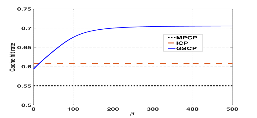
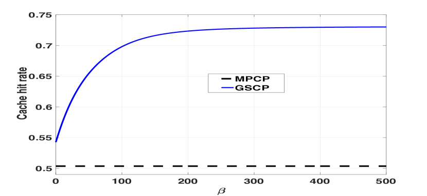
Figure 2: Comparison of Gibbs sampling based caching strategy, independent content placement strategy, and most popular content placement strategy, for a network with six BSs, four possible contents, and storage capacity for two contents in each BS cache. Detailed system parameters can be found in Section VI-D. The figure on the left is for scenario $1$ and the figure on the right are for scenario $2$ as described in Section VI-D

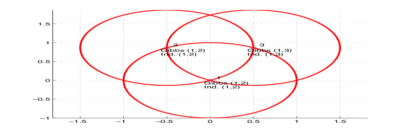
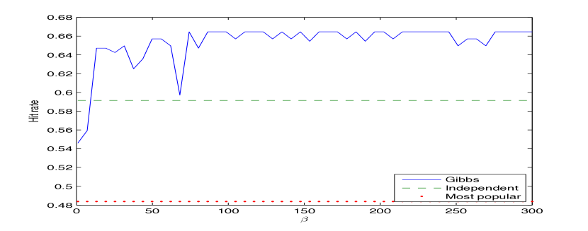
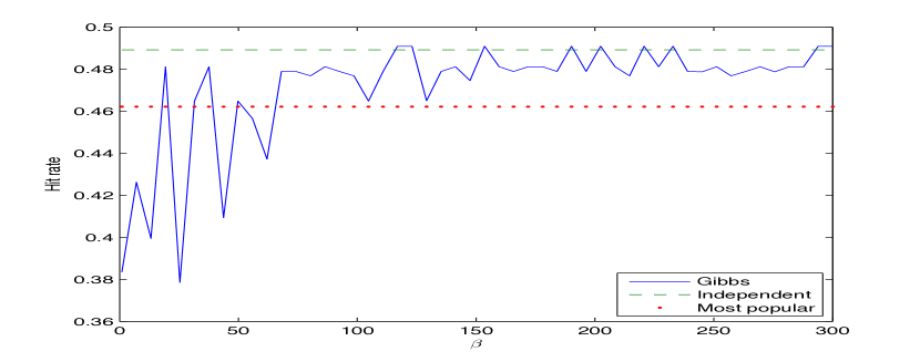
Figure 3: Comparison of Gibbs sampling based caching with only $100$ iterations, against independent content placement strategy, and most popular content placement strategy, for three BSs, five possible contents, and storage capacity of two contents per cache. Content popularities come from from Zipf distribution with parameter $\gamma=1.1$. Details can be found in Section VI-E. The top-left diagram shows more overlap among cells, whereas the top-right diagram shows less overlap. The diagrams at the bottom row correspond to the performance comparison among algorithms for these two cases.

VI-E Effect of finite number of iterations, $\beta$, and cell overlap

In this subsection, we demonstrate the caching performance of Gibbs sampling with only a finite number of iterations. We consider two different cases: (i) three base stations on the plane, each with unit radius, more overlap among cells, and (ii) three base stations on the plane, each with unit radius, less overlap among cells. The set of contents are $\mathcal{M}=\{1,2,3,4,5\}$ with their popularities coming from a Zipf distribution with parameter $\gamma=1.1$. Each cache can store at most two contents (i.e., $K=2$).

For these two cases, for various values of $\beta$, we simulated the Gibbs sampling algorithm (Algorithm 1) for $100$ iterations, noted the configuration obtained after the $100$-th iteration, and computed the cache hit rates for these configurations via simulation. Next, we compared them against cache hit rates for most popular content placement and independent content placement schemes. The results are summarized in Figure 3, where hit rates are computed per unit area of the entire window and not over the region covered by base stations alone. By the discussion provided in Section VI-B, we can expect that Gibbs sampling and independent content placement algorithms are both optimal if the cells become more overlapping. It is indeed seen in Figure 3 that the performances of Gibbs sampling and independent content placement algorithms are much better than most popular content placement, in case there is more overlapping among cells. It is also seen that the performance of Gibbs sampling tends to be better than independent content placement algorithm for large $\beta$. However, it is important to remember that we have only provided result for one sample path for each $\beta$; since we have taken only $100$ iterations for Gibbs sampling, the results will vary if another independent sample path is chosen for the Gibbs sampling algorithm. Hence, Figure 3 only demonstrates the potential performance improvement by Gibbs sampling over finite time; on the other hand, Section VI-D demonstrates that Gibbs sampling asymptotically achieves higher hit rate than independent content placement strategy and most popular content placement strategy.

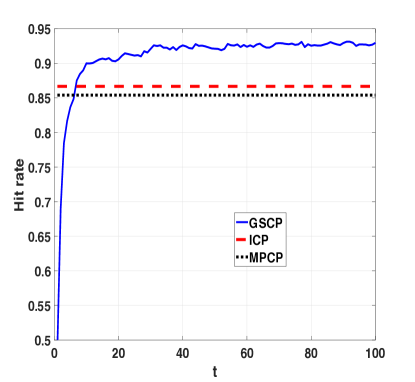
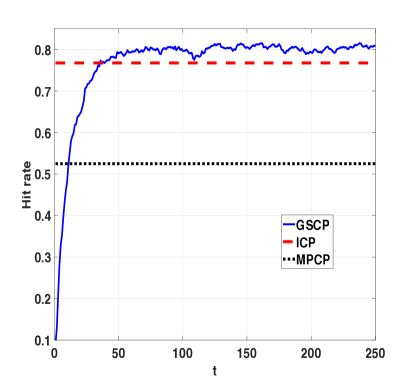
Figure 4: Demonstration of convergence speed of GSCP under $\beta=150$, and performance improvement over ICP and MPCP. Left: $N=5$, $M=5$, $K=2$, Zipf popularity distribution with parameter $\gamma=2$, averaged over $10$ sample paths. Right: $N=20$, $M=14$, $K=5$, Zipf popularity distribution with parameter $\gamma=0.5$, averaged over $4$ sample paths. Details are provided in Section VI-F.

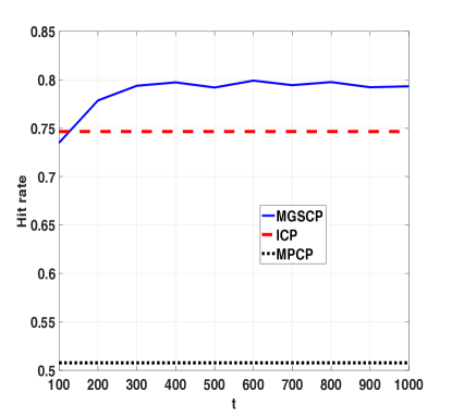
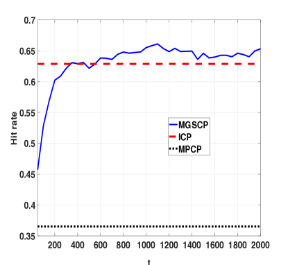
Figure 5: Demonstration of convergence speed of modified GSCP (MGSCP), and performance improvement over ICP and MPCP. Left: $N=20$, $M=50$, $K=15$, random popularity distribution, $\beta=1000$, averaged over $4$ sample paths. Right: $N=20$, $M=100$, $K=20$, random popularity distribution, $\beta=2000$, single sample path. For MGSCP, all caches initially start with $K$ most popular contents. Details are provided in Section VI-F.

VI-F Numerical example for mixing time and performance improvement of Gibbs sampling

Now we demonstrate the speed of convergence of Gibbs sampling for fixed $\beta$. Location of $N$ base stations are generated independently with uniform distribution over the unit square, and the cell radius is assumed to be $\sqrt{\frac{5}{\textbullet\pi N}}$. Popularities of $M$ contents are generated either independently with uniform distribution, or they are assumed to follow Zipf distribution with parameter $\gamma$.

Results for small system size: For GSCP, each cache is assumed to be empty at $t=0$. The performance of GSCP for $\beta=150$, averaged over multiple independent sample paths, is compared against MPCP and ICP for various values of $N$, $M$ and the cache size $K$; for GSCP, at each $t$, hit rate for the current cache configuration is considered. Cache hit rate under GSCP is plotted against $t$ in Figure 4. The results show that, GSCP outperforms MPCP and ICP significantly and reaches stationary distribution for even $t\leq 50$ if $N=5$; for $N=20$, the stationary distribution is nearly achieved starting from $t=100$. Of course, the convergence will be slower if $N$, $M$ and $K$ are increased further; for large values of $N$, $M$ and $K$, one can simply use GSCP with only highly popular contents (for example, most popular contents whose collective popularity is $0.95$ or above).

Results for large system size: As discussed in Remark 2, the $O({{M}\choose{K}})$ computations per iteration in Gibbs sampling (using (8)) can be prohibitive for GSCP to be applied to a large scale system. We alleviate this problem by proposing a simple modified GSCP algorithm (which we call MGSCP) where, at each iteration, only one randomly selected content is removed from a randomly selected BS, and then it is replaced by one content (absent in the cache after the removal) randomly via Gibbs sampling; thus, the denominator in (8) is replaced by a summation over all $(M-K+1)$ configurations that can possibly result via this replacement operation. Clearly this requires only $O(M-K+1)$ computations per iteration of Gibbs sampling and hence is easily implementable. This might reduce the convergence speed, but that can be compensated if one runs this iteration multiple times between two successive discrete time instants. However, here we assume that this update is done only once at each $t$. To reduce computation, we compute the hit rate only when $t$ is an integer multiple of either $50$ or $100$. Figure 5 demonstrates that the MGSCP algorithm may take at most a few hundred iterations before it starts outperforming ICP, and the convergence to steady state distribution is also clear from the plots; a few hundred iterations is not big for this large scale system (with $N=20$ and $M=50$ or $100$), especially keeping in mind that multiple iterations can be performed in practice between two successive decision instants. Thus, MGSCP provides a fast, distributed, optimal algorithm for content placement in a large system.

VII Conclusion

In this paper, we have provided algorithms for cache content update in a cellular network, motivated by Gibbs sampling techniques. The algorithms were shown to converge asymptotically to the optimal content placement in the caches. It turns out that the computation and communication cost is affordable for practical cellular network base stations.

While the current paper solves an important problem, there are still possibilities for numerous interesting extensions: (i) We assumed uniform download cost from the backhaul network for all base stations. However, this is not in general true. Depending on the backhaul architecture, backhaul link capacities and congestion scenario, it might be more desirable to avoid download from some specific base stations. Even different base stations might have different link capacities, and in practice, this will result in queueing delay for the download process. Contents might be of various classes, and hence may not have fixed size. Hence, a combined formulation of cache update and backhaul network state evolution will be necessary. (ii) Different cells might witness different content popularities, but this has not been addressed in the current paper. (iii) Once a content becomes irrelevant (e.g., a news video), it has to be removed completely from all caches; one needs to develop techniques to detect when to remove a content from all caches. (iv) Providing convergence rate guarantees when the inverse temperature is increasing and when arrival rates and cell topology are learnt over time, is a very challenging problem. We leave these issues for future research endeavours on this topic.

Arpan Chattopadhyay obtained his B.E. in Electronics and Telecommunication Engineering from Jadavpur University, Kolkata, India in the year 2008, and M.E. and Ph.D in Telecommunication Engineering from Indian Institute of Science, Bangalore, India in the year 2010 and 2015, respectively. He is currently working in the Ming Hsieh Department of Electrical Engineering, University of Southern California, Los Angeles as a postdoctoral researcher. Previously he worked as a postdoc in INRIA/ENS Paris. His research interests include wireless networks, cyber-physical systems, machine learning and control.

Bartlomiej Blaszczyszyn received his PhD degree and Habilitation qualification in applied mathematics from University of Wroclaw (Poland) in 1995 and 2008, respectively. He is now a Senior Researcher at Inria (France), and a member of the Computer Science Department of Ecole Normale Superieure in Paris. His professional interests are in applied probability, in particular in stochastic modeling and performance evaluation of communication networks. He coauthored several publications on this subject in major international journals and conferences, as well as a two-volume book on Stochastic Geometry and Wireless Networks NoW Publishers, jointly with F. Baccelli.

H. Paul Keeler graduated in physics and applied mathematics in 2006 from Griffith University. He received a Ph.D. in applied mathematics in 2010 from the University of Melbourne. After stints as a consultant in market research and banking and a guest researcher at the University of Zaragoza, Spain, he worked for two years as a researcher at Inria and École Normale Supérieure, Paris, where he was partly funded by Orange Labs. Currently he is a researcher at Weierstrass Institute (or WIAS), Berlin. His research interests lie in applied probability, numerical and asymptotic methods, communication networks.

Appendix A Definition of weak and strong ergodicity

Let us consider a discrete-time inhomogeneous Markov chain $\{X(t)\}_{t\geq 0}$ whose transition probability matrix (t.p.m.) between $t=m$ and $t=m+n$ is given by $P(m;n)$. Let $\mathcal{D}$ be the collection of all possible distributions (each element in $\mathcal{D}$ is assumed to be a row vector) on the state space. Then $\{X(t)\}_{t\geq 0}$ is called weakly ergodic if, for all $m\geq 0$,

$$\lim_{n\uparrow\infty}\sup_{\mu,\nu\in\mathcal{D}}d_{V}(\mu P(m;n),\nu P(m;n))=0,$$

where $d_{V}(\cdot,\cdot)$ is the total variation distance between two distributions.

$\{X(t)\}_{t\geq 0}$ is called strongly ergodic if there exists $\pi\in\mathcal{D}$ such that, for all $m\geq 0$,

$$\lim_{n\uparrow\infty}\sup_{\mu\in\mathcal{D}}d_{V}(\mu^{T}P(m;n),\pi)=0.$$

Appendix B Proof of Theorem 1

Fix a small $\epsilon>0$. Under configuration $B$ of the virtual caches, let us denote the total time $T_{B}$ (a generic random variable) taken by the arrival process so that, for all possible pairs $(i,j)\in\{1,2,\cdots,M\}\times\{1,2,\cdots,N\}$ there is at least one request for content $i$ to BS $j$ if virtual configuration $B$ suggests placing content $i$ at BS $j$; clearly $\mathbf{E}(T_{B})<\infty$, since we have made Assumption 1. Let us consider $l\in\mathbb{Z}_{+}$ large enough such that: (i) $\sum_{B\in\mathcal{B}}|\mathbf{P}(V(t)=B)-\pi_{\beta}(B)|<\epsilon$ for all integer $t\geq S_{l-1}$, (ii) $\mathbf{P}(T_{B}>\epsilon T_{l+1})<\epsilon$.

Now,

$$\frac{\int_{S_{l}}^{S_{l+1}}\mathbf{P}(R(\tau)=B)d\tau}{T_{l+1}}$$

$$\geq \frac{\mathbf{E}\int_{\min\{S_{l}+T_{B}^{{}^{\prime}},S_{l+1}\}}^{S_{l+1}}\mathbf{P}(R(\tau)=B)d\tau}{T_{l+1}}$$

$$\geq \frac{\mathbf{P}(T_{B}^{{}^{\prime}}\leq\epsilon T_{l+1})\mathbf{E}\bigg{(}\int_{\min\{S_{l}+T_{B}^{{}^{\prime}},S_{l+1}\}}^{S_{l+1}}\mathbf{P}(R(\tau)=B)d\tau\bigg{|}T_{B}^{{}^{\prime}}\leq\epsilon T_{l+1}\bigg{)}}{T_{l+1}}$$

$$\geq \frac{(1-\epsilon)\int_{S_{l}+\epsilon T_{l+1}}^{S_{l+1}}\mathbf{P}(R(\tau)=B|T_{B}^{{}^{\prime}}\leq\epsilon T_{l+1})d\tau}{T_{l+1}}$$

$$= \frac{(1-\epsilon)(T_{l+1}-\epsilon T_{l+1})\mathbf{P}(V(S_{l}-)=B)}{T_{l+1}}$$

$$\geq (1-\epsilon)^{2}(\pi_{\beta}(B)-\epsilon),$$

where $T_{B}^{{}^{\prime}}$ has the same distribution as $T_{B}$. The equality step follows from the fact that for $\tau>S_{l}+\epsilon T_{l+1}$, we have $\mathbf{P}(R(\tau)=B|T_{B}^{{}^{\prime}}\leq\epsilon T_{l+1})=V(S_{l}-)$, since all real caches are updated to $V(S_{l}-)$ within $\tau\leq S_{l}+T_{B}^{{}^{\prime}}$.

Hence,

$$\liminf_{T\rightarrow\infty}\frac{\int_{0}^{T}\mathbf{P}(R(\tau)=B)d\tau}{T}$$

$$= \liminf_{T\rightarrow\infty}\frac{\int_{S_{l}}^{T}\mathbf{P}(R(\tau)=B)d\tau}{T-S_{l}}$$

$$\geq (1-\epsilon)^{2}(\pi_{\beta}(B)-\epsilon).$$

Since $\epsilon>0$ is arbitrarily small, we have:

$$\liminf_{T\rightarrow\infty}\frac{\int_{0}^{T}\mathbf{P}(R(\tau)=B)d\tau}{T}\geq\pi_{\beta}(B).$$

But, by Fatou’s lemma (see [34, Chapter $4$]),

$$\sum_{B\in\mathcal{B}}\liminf_{T\rightarrow\infty}\frac{\int_{0}^{T}\mathbf{P}(R(\tau)=B)d\tau}{T}$$

$$\leq \liminf_{T\rightarrow\infty}\sum_{B\in\mathcal{B}}\frac{\int_{0}^{T}\mathbf{P}(R(\tau)=B)d\tau}{T}=1$$

and $\sum_{B\in\mathcal{B}}\pi_{\beta}(B)=1$. Hence, we must have $\liminf_{T\rightarrow\infty}\frac{\int_{0}^{T}\mathbf{P}(R(\tau)=B)d\tau}{T}=\pi_{\beta}(B)$ for all $B\in\mathcal{B}$.

On the other hand,

$$\limsup_{T\rightarrow\infty}\frac{\int_{0}^{T}\mathbf{P}(R(\tau)=B)d\tau}{T}=\limsup_{l\rightarrow\infty}\frac{\int_{S_{l}}^{S_{l+1}}\mathbf{P}(R(\tau)=B)d\tau}{T_{l+1}}.$$

Now,

$$\frac{\int_{S_{l}}^{S_{l+1}}\mathbf{P}(R(\tau)=B)d\tau}{T_{l+1}}$$

$$\leq \frac{\int_{S_{l}+\epsilon T_{l+1}}^{S_{l+1}}\mathbf{P}(R(\tau)=B)d\tau+\epsilon T_{l+1}}{T_{l+1}}$$

$$\leq \frac{\int_{S_{l}+\epsilon T_{l+1}}^{S_{l+1}}\mathbf{P}(R(\tau)=B|T_{B}^{{}^{\prime}}\leq\epsilon T_{l+1})d\tau+2\epsilon T_{l+1}}{T_{l+1}}$$

$$\leq \frac{\int_{S_{l}+\epsilon T_{l+1}}^{S_{l+1}}\mathbf{P}(V(S_{l}-)=B)d\tau+2\epsilon T_{l+1}}{T_{l+1}}$$

$$\leq \pi_{\beta}(B)+3\epsilon,$$

where the second inequality follows from the fact that for $\tau\in[S_{l}+\epsilon T_{l+1},S_{l+1})$:

$$\mathbf{P}(R(\tau)=B)$$

$$\leq \mathbf{P}(R(\tau)=B|T_{B}^{{}^{\prime}}\leq\epsilon T_{l+1})$$

$$+\mathbf{P}(T_{B}^{{}^{\prime}}>\epsilon T_{l+1})\mathbf{P}(R(\tau)=B|T_{B}^{{}^{\prime}}>\epsilon T_{l+1})$$

$$\leq \mathbf{P}(R(\tau)=B|T_{B}^{{}^{\prime}}\leq\epsilon T_{l+1})+\epsilon.$$

Since $\epsilon>0$ is arbitrarily small, we can say that: $\limsup_{T\rightarrow\infty}\frac{\int_{0}^{T}\mathbf{P}(R(\tau)=B)d\tau}{T}\leq\pi_{\beta}(B).$

Hence, $\lim_{T\rightarrow\infty}\frac{\int_{0}^{T}\mathbf{P}(R(\tau)=B)d\tau}{T}=\pi_{\beta}(B)$.

Appendix C Proof of Theorem 2

In this proof, we will use the notion of weak and strong ergodicity of time-inhomogeneous Markov chains from [32, Chapter $6$, Section $8$]), which is provided in Appendix A.

Fix $k=0$. We will first show that the Markov chain $\{V(t)\}_{t\geq 0}$ in weakly ergodic.

Let us consider the transition probability matrix (t.p.m.) $Q_{l}$ for the inhomogeneous Markov chain $\{Y(l)\}_{l\geq 0}$, where $Y(l):=V(lN)$. Then, the Dobrushin’s ergodic coefficient $\delta(Q_{l})$ is given by (see [32, Chapter $6$, Section $7$] for definition) $\delta(Q_{l})=1-\inf_{B^{{}^{\prime}},B^{{}^{\prime\prime}}\in\mathcal{B}}\sum_{B\in\mathcal{B}}\min\{Q_{l}(B^{{}^{\prime}},B),Q_{l}(B^{{}^{\prime\prime}},B)\}$. The Markov chain $\{V(t)\}_{t\geq 0}$ is weakly ergodic if $\sum_{l=1}^{\infty}(1-\delta(Q_{l}))=\infty$ (by [32, Chapter $6$, Theorem $8.2$]).

Now, with positive probability, virtual caches in all nodes are updated over a period of $N$ slots. Hence, any $B\in\mathcal{B}$ can be reached over a period of $N$ slots, starting from any other $B^{{}^{\prime}}\in\mathcal{B}$. Note that, once a base station $j_{t}$ is chosen in Algorithm 1 at discrete time $t\in\{lN,lN+1,\cdots,lN+N-1\}$, the sampling probability for any set of contents in its virtual cache in a slot is lower bounded by $\frac{e^{-\beta_{t}\Delta}}{{{M}\choose{K}}}\geq\frac{e^{-\beta_{lN+N}\Delta}}{{{M}\choose{K}}}$, since $t<lN+N$. Hence, for independent sampling over $N$ slots, we will always have $Q_{l}(B^{{}^{\prime}},B)\geq\bigg{(}\frac{e^{-\beta_{lN+N}\Delta}}{N{{M}\choose{K}}}\bigg{)}^{N}>0$ for all pairs $B^{{}^{\prime}},B$. Hence,

$$\sum_{l=0}^{\infty}(1-\delta(Q_{l}))$$ (11)

$$= \sum_{l=0}^{\infty}\inf_{B^{{}^{\prime}},B^{{}^{\prime\prime}}\in\mathcal{B}}\sum_{B\in\mathcal{B}}\min\{Q_{l}(B^{{}^{\prime}},B),Q_{l}(B^{{}^{\prime\prime}},B)\}$$

$$\geq \sum_{l=0}^{\infty}\sum_{B\in\mathcal{B}}\bigg{(}\frac{e^{-\beta_{0}\log(1+lN+N)\times\Delta}}{N{{M}\choose{K}}}\bigg{)}^{N}$$

$$= {{M}\choose{K}}^{N}\times\frac{1}{(N{{M}\choose{K}})^{N}}\sum_{l=0}^{\infty}e^{-N\Delta\beta_{0}\log(1+lN+N)}$$

$$= \frac{1}{N^{N}}\sum_{l=0}^{\infty}\frac{1}{(1+lN+N)^{\beta_{0}N\Delta}}$$

$$\geq \frac{1}{N^{N}}\frac{1}{N}\sum_{t=N+1}^{\infty}\frac{1}{(1+t)^{\beta_{0}N\Delta}}$$

$$= \infty.$$

Here the last step follows from the fact that $\sum_{t=1}^{\infty}\frac{1}{t^{a}}$ diverges for $0<a<1$. The second equality follows from the fact that there are ${{M}\choose{K}}^{N}$ possible configurations.

Hence, the Markov chain $\{V(t)\}_{t\geq 0}$ is weakly ergodic.

Now we will use [32, Chapter $6$, Theorem $8.3$] to prove strong ergodicity of $\{V(t)\}_{t\geq 0}$.

Let us denote the t.p.m. of $\{V(t)\}_{t\geq 0}$ at a specific time $t=T$ by $Q^{(T)}$ (a specific matrix). If the Markov chain $\{V(t)\}_{t\geq 0}$ is allowed to evolve up to infinite time with fixed t.p.m. $Q^{(T)}$, then we will get stationary distribution $\pi_{\beta_{T}}(B)=\frac{e^{\beta_{T}h(B)}}{Z_{\beta_{T}}}$. This satisfies Condition $8.9$ of [32, Chapter $6$, Theorem $8.3$].

Now we will check Condition $8.10$ of [32, Chapter $6$, Theorem $8.3$]. For any $B\in\arg\max_{B^{{}^{\prime}}\in\mathcal{B}}h(B^{{}^{\prime}})$, it is easy to see that $\pi_{\beta_{T}}(B)$ increases with $T$ for large $T$ (can be seen by considering derivative of $\pi_{\beta}(B)$ w.r.t. $\beta$). For all other configurations $B$, $\pi_{\beta_{T}}(B)$ decreases with $T$ for large $T$. Hence, $\sum_{T=0}^{\infty}\sum_{B\in\mathcal{B}}|\pi_{\beta_{T+1}}(B)-\pi_{\beta_{T}}(B)|<\infty$. In order to see this, let us assume without loss of generality that, $B\in\arg\max_{B^{{}^{\prime}}\in\mathcal{B}}h(B^{{}^{\prime}})$ so that $\pi_{\beta_{T}}(B)$ monotonically increases with $T$ for all $T\geq T^{{}^{\prime}}$. But $0\leq\pi_{\beta_{T}}(B)\leq 1$ for all $T$. Hence, $\{\pi_{\beta_{T}}(B)\}_{T\geq 1}$ converges and $\sum_{T=T^{{}^{\prime}}}^{\infty}|\pi_{\beta_{T+1}}(B)-\pi_{\beta_{T}}(B)|=\sum_{T=T^{{}^{\prime}}}^{\infty}(\pi_{\beta_{T+1}}(B)-\pi_{\beta_{T}}(B))=\lim_{T\rightarrow\infty}\pi_{\beta_{T}}(B)-\pi_{\beta_{T^{{}^{\prime}}}}(B)<\infty$. Similar claims can be made for all $B\in\mathcal{B}$. Hence, we can claim that $\sum_{T=0}^{\infty}\sum_{B\in\mathcal{B}}|\pi_{\beta_{T+1}}(B)-\pi_{\beta_{T}}(B)|<\infty$.

Hence, by [32, Chapter $6$, Theorem $8.3$], $\{V(t)\}_{t\geq 0}$ is strongly ergodic. The expression for the limiting distribution is straightforward to derive.

Appendix D Proof of Theorem 4

Note that, at a given fixed time $t=T$, given the instantaneous value of estimates, the instantaneous transition probability matrix for $\{V(t)\}_{t\geq 0}$ Markov chain, $Q^{(T)}$, will have a stationary probability distribution. Also, if we assume that there exists exactly one configuration in the set $\arg\max_{B\in\mathcal{B}}h(B)$, then we can say that $\lim_{T\rightarrow\infty}|Q^{(T)}-Q^{*}|=0$, where $Q^{*}$ has a stationary distribution which assigns probability $1$ on $\arg\max_{B\in\mathcal{B}}h(B)$, and $Q^{*}$ is ergodic. Hence, by [32, Chapter $6$, Theorem $8.5$], the Markov chain $\{V(t)\}_{t\geq 0}$ is strongly ergodic.

References

- [1] B. Blaszczyszyn and H.P. Keeler. Studying the sinr process of the typical user in poisson networks using its factorial moment measures. IEEE Transactions on Information Theory, 61(12):6774–6794, 2015.
- [2] B. Blaszczyszyn and A. Giovanidis. Optimal geographic caching in cellular networks. In IEEE International Conference on Communications (ICC), pages 3358–3363, 2015.
- [3] K. Shanmugam, N. Golrezaei, A. G. Dimakis, A. F. Molisch, and G. Caire. Femtocaching: Wireless content delivery through distributed caching helpers. IEEE Transactions on Information Theory, 59(12):8402–8413, 2013.
- [4] Fan Xu, Kangqi Liu, and Meixia Tao. Cooperative tx/rx caching in interference channels: A storage-latency tradeoff study. In Information Theory (ISIT), 2016 IEEE International Symposium on, pages 2034–2038. IEEE, 2016.
- [5] Zheng Chen, Jemin Lee, Tony QS Quek, and Marios Kountouris. Cooperative caching and transmission design in cluster-centric small cell networks. IEEE Transactions on Wireless Communications, 16(5):3401–3415, 2017.
- [6] X. Wang, M. Chen, T. Taleb, A. Ksentini, and V. Leung. Cache in the air: Exploiting content caching and delivery techniques for 5g systems. IEEE Communications Magazine, 52(2):131–139, 2014.
- [7] V. Martina, M. Garetto, and E. Leonardi. A unified approach to the performance analysis of caching systems. In IEEE Conference on Computer Communications (INFOCOM), pages 2040–2048, 2014.
- [8] K. Poularakis and L. Tassiulas. Exploiting user mobility for wireless content delivery. In International Symposium on Information Theory (ISIT), pages 1017–1021, 2013.
- [9] Berksan Serbetci and Jasper Goseling. On optimal geographical caching in heterogeneous cellular networks. In Wireless Communications and Networking Conference (WCNC), 2017 IEEE, pages 1–6. IEEE, 2017.
- [10] Dong Liu and Chenyang Yang. Caching policy toward maximal success probability and area spectral efficiency of cache-enabled hetnets. IEEE Transactions on Communications, 2017.
- [11] Konstantin Avrachenkov, Xinwei Bai, and Jasper Goseling. Optimization of caching devices with geometric constraints. arXiv preprint arXiv:1602.03635, 2016.
- [12] K. Hamidouche, W. Saad, M. Debbah, and H.V. Poor. Mean-field games for distributed caching in ultra-dense small cell networks. In American Control Conference (ACC), pages 4699–4704, 2016.
- [13] KP Naveen, Laurent Massoulie, Emmanuel Baccelli, Aline Carneiro Viana, and Don Towsley. On the interaction between content caching and request assignment in cellular cache networks. In Proceedings of the 5th Workshop on All Things Cellular: Operations, Applications and Challenges, pages 37–42. ACM, 2015.
- [14] F. Pantisano, Mehdi Bennis, Walid Saad, and Merouane Debbah. In-network caching and content placement in cooperative small cell networks. In International Conference on 5G for Ubiquitous Connectivity, pages 128–133. IEEE, 2014.
- [15] Y.H. Chiang and W. Liao. Encore: An energy-aware multicell cooperation in heterogeneous networks with content caching. In IEEE International Conference on Computer Communications (INFOCOM), pages 1–9. IEEE, 2016.
- [16] Ammar Gharaibeh, Abdallah Khreishah, Bo Ji, and Moussa Ayyash. A provably efficient online collaborative caching algorithm for multicell-coordinated systems. IEEE Transactions on Mobile Computing, 15(8):1863–1876, 2016.
- [17] P. Ostovari, J. Wu, and A. Khreishah. Efficient online collaborative caching in cellular networks with multiple base stations. In IEEE 13th International Conference on Mobile Ad Hoc and Sensor Systems (MASS). IEEE, 2016.
- [18] W. Jiang, G. Feng, and S. Qin. Optimal cooperative content caching and delivery policy for heterogeneous cellular networks. IEEE Transactions on Mobile Computing, IEEE Early Access Articles, PP(99):1–1.
- [19] Konstantin Avrachenkov, Jasper Goseling, and Berksan Serbetci. A low-complexity approach to distributed cooperative caching with geographic constraints. Proceedings of the ACM on Measurement and Analysis of Computing Systems, 1(1):27, 2017.
- [20] E. Bastug, M. Bennis, and M. Debbah. Cache-enabled small cell networks: Modeling and tradeoffs. In International Symposium on Wireless Communications Systems (ISWCS), pages 649–653. IEEE, 2014.
- [21] E. Bastug, M. Kountouris M. Bennis, and M. Debbah. Edge caching for coverage and capacity-aided heterogeneous networks. In International Symposium on Information Theory (ISIT), pages 285–289. IEEE, 2016.
- [22] M. Kountouris E. Bastug, M. Bennis, and M. Debbah. On the delay of geographical caching methods in two-tiered heterogeneous networks. In International Workshop on Signal Processing Advances in Wireless Communications (SPAWC), pages 1–5. IEEE, 2016.
- [23] B.N. Bharath, K.G. Nagananda, and H. V. Poor. A learning-based approach to caching in heterogenous small cell networks. IEEE Transactions on Communications, 64(4):1674–1686, 2016.
- [24] M. Leconte, G. Paschos, L. Gkatzikis, M. Draief, S. Vassilaras, and S. Chouvardas. Placing dynamic content in caches with small population. In IEEE International Conference on Computer Communications (INFOCOM), pages 1–9, 2016.
- [25] S. Moharir, J. Ghaderi, S. Sanghavi, and S. Shakkottai. Serving content with unknown demand: the high-dimensional regime. In ACM international conference on Measurement and modeling of computer systems (SIGMETRICS), pages 435–447, 2014.
- [26] E. Bastug, M. Bennis, E. Zeydan, M. Abdel Kader, A. Karatepe, A. Salih Er, and M. Debbah. Big data meets telcos: A proactive caching perspective. Journal of Communications and Networks, 17(6):549–557, 2015.
- [27] Giovanni Neglia, Damiano Carra, and Pietro Michiardi. Cache policies for linear utility maximization. PhD thesis, Inria Sophia Antipolis, 2017.
- [28] G. Paschos, E. Bastug, I. Land, G. Caire, and M. Debbah. Wireless caching: technical misconceptions and business barriers. IEEE Communications Magazine, 4(8):16–22, 2016.
- [29] A. Sengupta, S.D. Amuru, R. Tandon, R.M. Buehrer, and T.C. Clancy. Learning distributed caching strategies in small cell networks. In International Symposium on Wireless Communications Systems (ISWCS), pages 917–921. IEEE, 2014.
- [30] R. Tandon and O. Simeone. Cloud-aided wireless networks with edge caching: Fundamental latency trade-offs in fog radio access networks. In International Symposium on Information Theory (ISIT), pages 2029–2033. IEEE, 2016.
- [31] R.M. Karp. Reducibility among combinatorial problems. Complexity of computer computations, pages 85–103, 1972.
- [32] P. Bremaud. Markov Chains, Gibbs Fields, Monte Carlo Simulation, and Queues. Springer, 1999.
- [33] Bruce Hajek. Cooling schedules for optimal annealing. Mathematics of operations research, 13(2):311–329, 1988.
- [34] H.L. Royden and P.M. Fitzpatrick. Real Analysis (Fourth Edition). Pearson Education Asia Limited and China Machine Press, 2010.