Scalar field self-force effects on a particle orbiting a Reissner-Nordström black hole

Abstract

Scalar field self-force effects on a scalar charge orbiting a Reissner-Nordström black hole are investigated. The scalar wave equation is solved analytically in a post-Newtonian framework, and the solution is used to compute the self-field as well as the components of the self-force at the particle’s location up to 7.5 post-Newtonian order. The energy fluxes radiated to infinity and down the hole are also evaluated. Comparison with previous numerical results in the Schwarzschild case shows a good agreement in both strong-field and weak-field regimes.

I Introduction

Scalar self-force (SSF) effects arise when a scalar charge, moving along a given orbit in a curved spacetime, interacts with its own gravitational field, i.e., its self-field. The associated scalar field satisfies a d’Alembert-like equation with source term singular at the particle’s position, mimicking the more interesting situation of gravitational perturbations induced by a small mass moving in a gravitational background modified by its own presence. The interaction of the particle with its own gravitational field in this case gives rise to a gravitational self-force (GSF) (see, e.g., Ref. Barack:2009ux and references therein). It is a matter of fact that the latter problem is physically more interesting than the first one. However, the study of the first problem is easier than the second, even if the approaches as well as the computational techniques used in both cases are similar. This explains why in the literature the SSF problem has been considered as a preliminary study to the GSF one, scouting/solving all technical difficulties also affecting the more general gravitational perturbation problem. The existing literature on this topic is very rich. Indeed, besides the various pioneering works developing the fundamental formalism for self-force calculations in a curved spacetime Mino:1996nk ; Quinn:1996am ; Quinn:2000wa ; Barack:2001gx ; Barack:2001ph ; Detweiler:2002mi ; Poisson:2003nc , a number of interesting papers has been produced over the years, aiming at understanding self-force effects in black hole spacetimes, mostly Schwarzschild and Kerr Burko:1999zy ; Barack:2000eh ; Burko:2000xx ; Wiseman:2000rm ; Nakano:2001kw ; Burko:2001kr ; Barack:2002mha ; Detweiler:2002gi ; Nakano:2003he ; Hikida:2003pi ; DiazRivera:2004ik ; Hikida:2004hs ; Ottewill:2007mz ; Haas:2007kz ; Damour:2009sm ; Barack:2010tm ; Warburton:2010eq ; Warburton:2011hp ; Wardell:2011gb ; Ottewill:2012aj ; Vega:2013wxa ; Isoyama:2014mja ; Warburton:2014bya ; vandeMeent:2016pee .

The present paper concerns scalar field self-force effects in a Reissner-Nordström (RN) spacetime on a scalar charge moving along a spatially circular equatorial orbit around a spherically symmetric charged black hole. The interaction between the particle and the background field is thus of the gravitational type only, the particle carrying no electromagnetic charge. We are interested in studying the coupling between the scalar charge of the associated field with the mass and the electromagnetic charge of the non-vacuum background, which was never explored before. Switching off the black hole charge one ends up with the corresponding SSF problem in the vacuum Schwarzschild spacetime Nakano:2001kw ; Detweiler:2002gi ; DiazRivera:2004ik ; Hikida:2004hs .

The main technical difficulties associated with self-force calculations are related to the regularization procedure of the scalar field and its derivatives, allowing to extract the correct, physically meaningful self force components. We use the standard post-Newtonian (PN) expansion method to compute the self-field decomposed into spherical harmonics and frequency modes, and regularize it at the particle’s position mode by mode by subtracting the diverging large-$l$ limit. We analytically compute the regularized self-field as well as the components of the self-force up to 7.5PN order and compare our results with previous numerical studies in the Schwarzschild case DiazRivera:2004ik ; Warburton:2010eq , obtaining a good agreement also in the strong-field regime. Finally, we complete our analysis by providing explicit expressions for the scalar radiation both at infinity and on the outer horizon. Again, the comparison with previous numerical results in the Schwarzschild case Warburton:2010eq shows a good agreement.

II Scalar charge in a Reissner-Nordström background

Let us consider a Reissner-Nordström spacetime with line element written in standard Schwarzschild-like coordinates $(t,r,\theta,\phi)$ as

$$ds^{2}=-\frac{\Delta}{r^{2}}dt^{2}+\frac{r^{2}}{\Delta}dr^{2}+r^{2}(d\theta^{2}+\sin^{2}\theta d\phi^{2})\,,$$ (1)

where $\Delta=r^{2}-2Mr+Q^{2}$. The condition $\Delta=0$ defines the two horizons at radii $r_{\pm}=M\pm\sqrt{M^{2}-Q^{2}}\equiv M(1\pm\kappa)$, with $\kappa=\sqrt{1-Q^{2}/M^{2}}$. The “extreme” case corresponds to $|Q|=M$ (or $\kappa=0$), the two horizons coalescing into one. We find it convenient to introduce also the notation $w=1-\kappa^{2}=(Q/M)^{2}$, such that $w=0$ corresponds to the Schwarzschild limit, while $w=1$ to the extreme RN case.

Let $\psi$ be a (real, minimally coupled) scalar field associated with a scalar charge $q$ moving along a circular equatorial timelike geodesic with 4-velocity $U=\Gamma(\partial_{t}+\Omega\partial_{\phi})$ and parametric equations $x^{\mu}=z^{\mu}(\tau)$

$$t=\Gamma\tau\,,\qquad r=r_{0}\,,\qquad\theta=\frac{\pi}{2}\,,\quad\phi=\Gamma\Omega\tau=\Omega t\,,$$ (2)

where $\tau$ denotes the proper time, and the normalization factor $\Gamma$ and the angular velocity $\Omega$ are conveniently written in terms of the inverse dimensionless radial distance $u=M/r$ as

$$\Gamma = \frac{1}{\sqrt{1-3u+(1-\kappa^{2})u^{2}}}\,,$$

$$M\Omega = u^{3/2}\,\sqrt{1-(1-\kappa^{2})u}\,,$$ (3)

respectively.

Assuming that the particle’s field can be treated as a small perturbation on the fixed RN background implies that it obeys the massless Klein-Gordon equation

$$\square\psi=-4\pi\varrho\,,$$ (4)

where

$$\square\psi=\frac{1}{\sqrt{-g}}\partial_{\mu}(\sqrt{-g}g^{\mu\nu}\partial_{\nu}\psi)$$ (5)

is the D’Alembertian (with $g$ denoting the determinant of the metric) and

$$\varrho(x^{\mu}) = q\int{(-g)^{-1/2}\delta^{4}(x^{\mu}-z^{\mu}(\tau))}d\tau$$ (6)

$$= \frac{q}{r_{0}^{2}\Gamma}\delta(r-r_{0})\delta\left(\theta-\frac{\pi}{2}\right)\delta(\phi-\Omega t)\,,$$

the charge density of the scalar particle with support only along the particle’s world line (2). Decomposing into spherical harmonics then gives

$$\varrho=\frac{1}{4\pi r_{0}}\delta(r-r_{0})\sum_{lm}q_{lm}e^{-im\Omega t}Y_{lm}(\theta,\phi)\,,$$ (7)

where

$$q_{lm}=\frac{4\pi q}{r_{0}\Gamma}Y_{lm}^{*}(\pi/2,0)\,,$$ (8)

and similarly for the scalar field $\psi$, whose dependence on temporal, radial and angular variables can be separated as

$$\psi(t,r,\theta,\phi)=\frac{1}{2\pi}\int\sum_{lm}\psi_{lm\omega}(r)e^{-i\omega t}Y_{lm}(\theta,\phi)\,d\omega\,.$$ (9)

The wave equation (4) thus reduces to the following equation for the radial part

$${\mathcal{L}}_{(r)}(\psi_{lm\omega}(r))=S_{lm\omega}\delta(r-r_{0})\,,$$ (10)

with

$${\mathcal{L}}_{(r)}(\psi_{lm\omega}(r)) \equiv \frac{d^{2}}{dr^{2}}\psi_{lm\omega}(r)+\frac{2(r-M)}{\Delta}\frac{d}{dr}\psi_{lm\omega}(r)$$ (11)

$$+ \left[\frac{\omega^{2}r^{4}}{\Delta^{2}}-\frac{l(l+1)}{\Delta}\right]\psi_{lm\omega}(r)\,,$$

whereas

$$S_{lm\omega}=-2\pi\frac{r_{0}}{\Delta_{0}}q_{lm}\delta(\omega-m\Omega)\,,$$ (12)

with $\Delta_{0}=\Delta(r_{0})$, comes from taking the Fourier-transform of the charge density (7).

III Computation of the scalar field along the world line

The radial part of the scalar field is computed by using the Green function method as

$$\psi_{lm\omega}(r) = \int G_{lm\omega}(r,r^{\prime})\Delta(r^{\prime})S_{lm\omega}\delta(r^{\prime}-r_{0})dr^{\prime}$$ (13)

$$= G_{lm\omega}(r,r_{0})\Delta_{0}S_{lm\omega}\,,$$

where the Green function $G_{lm\omega}(r,r^{\prime})$ satisfies the equation ${\mathcal{L}}_{(r)}(G_{lm\omega}(r,r^{\prime}))=\Delta^{-1}(r^{\prime})\delta(r-r^{\prime})$. It reads as

$$G_{lm\omega}(r,r^{\prime}) = \frac{1}{W_{lm\omega}}\left[R_{\rm in}^{lm\omega}(r)R_{\rm up}^{lm\omega}(r^{\prime})H(r^{\prime}-r)\right.$$ (14)

$$\left.+R_{\rm in}^{lm\omega}(r^{\prime})R_{\rm up}^{lm\omega}(r)H(r-r^{\prime})\right]\,,$$

where $H(x)$ denotes the Heaviside step function, $R_{\rm in}^{lm\omega}(r)$ and $R_{\rm up}^{lm\omega}(r)$ are two independent homogeneous solutions of the radial wave equation having the correct behavior at the outer horizon and at infinity, respectively, and

$$W_{lm\omega}=\Delta(r)\left[R_{\rm in}^{lm\omega}(r)R^{\prime}{}_{\rm up}^{lm\omega}(r)-R^{\prime}{}_{\rm in}^{lm\omega}(r)R_{\rm up}^{lm\omega}(r)\right]$$ (15)

is the associated (constant) Wronskian. Substituting then into Eq. (9) gives

$$\psi(x^{\mu})=-\sum_{lm}G_{lm\omega}(r,r_{0})\Big{|}_{\omega=m\Omega}r_{0}q_{lm}e^{-im\Omega t}Y_{lm}(\theta,\phi)\,,$$ (16)

which, once evaluated along the particle world line (2), becomes

$$\psi_{0}=-\frac{4\pi q}{\Gamma}\sum_{lm}G_{lm\omega}(r_{0},r_{0})\Big{|}_{\omega=m\Omega}|Y_{lm}(\pi/2,0)|^{2}\,,$$ (17)

only depending on $r_{0}$. The above expression for $\psi_{0}$ actually requires taking the limit $r\to r_{0}^{\pm}$ properly, and must be suitably regularized in order to remove its singular part, because the field has a divergent behavior there.

In order to compute the Green function we have first to solve the homogeneous radial wave equation (10) up to a certain PN order to obtain the in and up solutions, which are of the form

$$R_{\rm in(PN)}^{lm\omega}(r) = r^{l}[1+A_{2}^{lm\omega}(r)\eta^{2}+A_{4}^{lm\omega}(r)\eta^{4}$$

$$+A_{6}^{lm\omega}(r)\eta^{6}+A_{8}^{lm\omega}(r)\eta^{8}+\ldots]\,,$$

$$R_{\rm up(PN)}^{lm\omega}(r) = R_{\rm in(PN)}^{-l-1m\omega}(r)\,.$$ (18)

However, these solutions do not automatically fulfill the correct boundary conditions. A consequence of this fact is the presence of diverging terms in the coefficients $A_{i}$ for certain values of $l$. Therefore, high-order PN solutions usually require using a technique first introduced by Mano, Suzuki and Takasugi (MST) Mano:1996mf ; Mano:1996vt . We will show some detail in Appendix A.

Turning then to Eq. (17), the sum over $m$ is straightforwardly computed by using standard formulas. Before summing over $l$, instead, one has to remove the divergent term for large $l$, i.e.,

$$\psi_{0}^{\rm reg}=\sum_{l}(\psi_{0}^{l}-B)\,.$$ (19)

The subtraction term turns out to be (in units of $q$)

$$B = u-\frac{1}{4}u^{2}+\left(\frac{9}{64}-\frac{3}{4}\kappa^{2}\right)u^{3}$$ (20)

$$+\left(-\frac{73}{32}\kappa^{2}+\frac{199}{256}\right)u^{4}$$

$$+\left(\frac{39625}{16384}-\frac{39}{64}\kappa^{4}-\frac{1425}{256}\kappa^{2}\right)u^{5}$$

$$+\left(-\frac{907}{256}\kappa^{4}-\frac{52585}{4096}\kappa^{2}+\frac{451007}{65536}\right)u^{6}$$

$$+\left(-\frac{1926415}{65536}\kappa^{2}-\frac{109317}{8192}\kappa^{4}\right.$$

$$\left.+\frac{20043121}{1048576}-\frac{171}{256}\kappa^{6}\right)u^{7}+O(u^{8})\,.$$

This can be shown to be the Taylor expansion of

$$B_{\rm analytic}=\frac{u}{\sqrt{1-3u}}\frac{\sqrt{1-\sigma}}{\Gamma}\frac{2}{\pi}{\rm EllipticK}(\sigma)\,,$$ (21)

where

$$\sigma=\frac{u[1+u(1-\kappa^{2})]}{1-2u+u^{2}(1-\kappa^{2})}\,.$$ (22)

It is useful to introduce the dimensionless angular velocity variable

$$y=(M\Omega)^{2/3}=u(1+wu)^{1/3}\,,$$ (23)

as from Eq. (II), with inverse relation

$$u = y-\frac{1}{3}wy^{2}+\frac{1}{3}w^{2}y^{3}-\frac{35}{81}w^{3}y^{4}+\frac{154}{243}w^{4}y^{5}$$ (24)

$$-w^{5}y^{6}+\frac{10868}{6561}w^{6}y^{7}+O(y^{8})\,,$$

where we recall $w=1-\kappa^{2}$.

By applying the MST technique Mano:1996mf ; Mano:1996vt to the multipoles up to $l=4$ (included), we get the following final result for the regularized field valid up to the 7.5 PN order

$$\psi_{0}^{\rm reg} = -y^{3}+\left[\frac{35}{18}+\left(-\frac{7}{32}+\frac{w}{32}\right)\pi^{2}-\frac{4}{3}\gamma-\frac{4}{3}\ln(2)-\frac{2}{3}\ln(y)\right]y^{4}$$ (25)

$$+\left[\frac{1141}{360}-\frac{35}{54}w+\left(\frac{29}{512}+\frac{97}{1536}w-\frac{w^{2}}{96}\right)\pi^{2}+\left(\frac{2}{3}-\frac{8}{9}w\right)\gamma+\left(-\frac{18}{5}-\frac{8}{9}w\right)\ln(2)+\left(\frac{1}{3}-\frac{4}{9}w\right)\ln(y)\right]y^{5}$$

$$+\left(-\frac{38}{45}+\frac{8}{45}w\right)\pi y^{11/2}$$

$$+\left[-\frac{23741}{1680}+\frac{4607}{540}w+\frac{23}{54}w^{2}+\left(-\frac{279}{1024}-\frac{397}{1536}w-\frac{11}{512}w^{2}+\frac{1}{96}w^{3}\right)\pi^{2}+\left(\frac{77}{6}-\frac{46}{9}w+\frac{4}{9}w^{2}\right)\gamma\right.$$

$$\left.+\left(\frac{1627}{42}-\frac{54}{5}w+\frac{4}{9}w^{2}\right)\ln(2)-\frac{729}{70}\ln(3)+\left(\frac{77}{12}-\frac{23}{9}w+\frac{2}{9}w^{2}\right)\ln(y)\right]y^{6}$$

$$+\left(-\frac{3}{35}-\frac{2696}{4725}w+\frac{16}{135}w^{2}\right)\pi y^{13/2}$$

$$+\left\{-\frac{1515589307}{27216000}+\frac{3098381}{378000}w-\frac{3497}{3240}w^{2}-\frac{793}{1458}w^{3}\right.$$

$$\left.+\left(-\frac{58}{45}+\frac{8}{45}w\right)(1-w)^{3/2}-\frac{2}{3}(2-w)(1-w)\ln(1-w)\right.$$

$$+\left(-\frac{6059603}{983040}+\frac{1892003}{983040}w+\frac{2287}{9216}w^{2}+\frac{871}{20736}w^{3}-\frac{35}{2592}w^{4}\right)\pi^{2}+\left(\frac{76585}{262144}-\frac{14281}{131072}w+\frac{2665}{262144}w^{2}\right)\pi^{4}$$

$$+\left[-\frac{5321}{900}+\frac{4312}{675}w-\frac{4}{27}w^{2}-\frac{112}{243}w^{3}+\left(\frac{152}{45}-\frac{32}{45}w\right)\gamma+\left(\frac{304}{45}-\frac{64}{45}w\right)\ln(2)+\left(\frac{152}{45}-\frac{32}{45}w\right)\ln(y)\right]\gamma$$

$$+\left[-\frac{1786621}{18900}+\frac{149404}{4725}w-\frac{8}{15}w^{2}-\frac{112}{243}w^{3}+\left(\frac{152}{45}-\frac{32}{45}w\right)\ln(2)+\left(\frac{152}{45}-\frac{32}{45}w\right)\ln(y)\right]\ln(2)$$

$$\left.+\left(\frac{12393}{140}-\frac{729}{35}w\right)\ln(3)-\frac{16}{3}\zeta(3)+\left[-\frac{10121}{1800}+\frac{4856}{675}w-\frac{38}{27}w^{2}-\frac{56}{243}w^{3}+\left(\frac{38}{45}-\frac{8}{45}w\right)\ln(y)\right]\ln(y)\right\}y^{7}$$

$$+\left(\frac{35633}{3780}-\frac{192541}{33075}w+\frac{5062}{4725}w^{2}-\frac{8}{135}w^{3}\right)\pi y^{15/2}+O(y^{8})\,.$$

In the Schwarzschild case (i.e., in the limit $w\to 0$) it reduces to

$$\psi_{0}^{\rm reg,\,schw} = -y^{3}+\left(\frac{35}{18}-\frac{7}{32}\pi^{2}-\frac{4}{3}\gamma-\frac{4}{3}\ln(2)-\frac{2}{3}\ln(y)\right)y^{4}+\left(\frac{1141}{360}+\frac{29}{512}\pi^{2}+\frac{2}{3}\gamma-\frac{18}{5}\ln(2)+\frac{1}{3}\ln(y)\right)y^{5}$$ (26)

$$-\frac{38}{45}\pi y^{11/2}$$

$$+\left(-\frac{23741}{1680}-\frac{279}{1024}\pi^{2}+\frac{77}{6}\gamma+\frac{1627}{42}\ln(2)-\frac{729}{70}\ln(3)+\frac{77}{12}\ln(y)\right)y^{6}$$

$$-\frac{3}{35}\pi y^{13/2}$$

$$+\left[-\frac{1515589307}{27216000}-\frac{6059603}{983040}\pi^{2}+\frac{76585}{262144}\pi^{4}+\left(-\frac{5321}{900}+\frac{152}{45}\gamma+\frac{304}{45}\ln(2)+\frac{152}{45}\ln(y)\right)\gamma\right.$$

$$\left.+\left(-\frac{1786621}{18900}+\frac{152}{45}\ln(2)+\frac{152}{45}\ln(y)\right)\ln(2)+\frac{12393}{140}\ln(3)-\frac{16}{3}\zeta(3)+\left(-\frac{10121}{1800}+\frac{38}{45}\ln(y)\right)\ln(y)\right]y^{7}$$

$$+\frac{35633}{3780}\pi y^{15/2}+O(y^{8})\,,$$

which was never shown before in the literature . Scalar self force effects on a Schwarzschild background was numerically studied in Ref. DiazRivera:2004ik . We show in Table 1 and in Fig. 1 the comparison between our analytical results and the numerical values mentioned above. The agreement is excellent (i.e., of the order $\sim 10^{-14}$) in the weak-field region, as expected, and also good enough (i.e., of the order $\sim 10^{-4}$) in the strong-field region.

In order to study the transcendental structure of the various PN orders, it is useful to replace ordinary logarithms by “eulerlogs,” i.e.,

$${\rm eulerlog}_{m}(x)=\gamma+\ln(2)+\frac{1}{2}\ln(y)+\ln(m)\,,\qquad m=1,2,3,\ldots\,,$$ (27)

first introduced in Ref. Damour:2008gu , so to absorb also the Euler $\gamma$ constant. We obtain

$$\psi_{0}^{\rm reg,\,schw} = -y^{3}+\left(\frac{35}{18}-\frac{7}{32}\pi^{2}-\frac{4}{3}{\rm eulerlog}_{1}(y)\right)y^{4}+\left(\frac{1141}{360}+\frac{29}{512}\pi^{2}+\frac{74}{15}{\rm eulerlog}_{1}(y)-\frac{64}{15}{\rm eulerlog}_{2}(y)\right)y^{5}$$ (28)

$$-\frac{38}{45}\pi y^{11/2}$$

$$+\left(-\frac{23741}{1680}-\frac{279}{1024}\pi^{2}-\frac{93}{35}{\rm eulerlog}_{1}(y)+\frac{544}{21}{\rm eulerlog}_{2}(y)-\frac{729}{70}{\rm eulerlog}_{3}(y)\right)y^{6}$$

$$-\frac{3}{35}\pi y^{13/2}$$

$$+\left[-\frac{1515589307}{27216000}-\frac{6059603}{983040}\pi^{2}+\frac{76585}{262144}\pi^{4}+\frac{16}{3}\gamma-\frac{16}{3}\zeta(3)-\frac{77879}{4725}{\rm eulerlog}_{1}(y)-\frac{78704}{945}{\rm eulerlog}_{2}(y)\right.$$

$$\left.+\frac{12393}{140}{\rm eulerlog}_{3}(y)+\frac{152}{45}{\rm eulerlog}_{1}^{2}(y)\right]y^{7}$$

$$+\frac{35633}{3780}\pi y^{15/2}+O(y^{8})\,.$$

Unfortunately, this replacement is not enough to completely remove the Euler $\gamma$ term at the order $O(y^{7})$, meaning that the transcendental structure is more involved than simple eulerlogs.

It is also interesting to study the behavior of this scalar field at the light-ring $y=1/3$. A simple numerical fit

$$\psi_{0}^{\rm reg,\,schw\,fit}=-\frac{y^{3}}{(1-3y)^{2}}(1-7.84y+47.36y^{2}-8.65y^{3}+81.77y^{3}\ln(y))$$ (29)

(with a maximal residual of about $2.4\times 10^{-4}$) suggests a blow up of the form $(1-3y)^{-2}$. However, this is an indication only, and a more conclusive statement requires strong field numerical data still currently unavailable.

Finally, in the extreme RN case (i.e., in the limit $w\to 1$) we have

$$\psi_{0}^{\rm reg,\,extr} = -y^{3}+\left(\frac{35}{18}-\frac{3}{16}\pi^{2}-\frac{4}{3}\gamma-\frac{4}{3}\ln(2)-\frac{2}{3}\ln(y)\right)y^{4}+\left(\frac{2723}{1080}+\frac{7}{64}\pi^{2}-\frac{2}{9}\gamma-\frac{202}{45}\ln(2)-\frac{1}{9}\ln(y)\right)y^{5}$$ (30)

$$-\frac{2}{3}\pi y^{11/2}$$

$$+\left(-\frac{78233}{15120}-\frac{555}{1024}\pi^{2}+\frac{49}{6}\gamma+\frac{17881}{630}\ln(2)-\frac{729}{70}\ln(3)+\frac{49}{12}\ln(y)\right)y^{6}$$

$$-\frac{121}{225}\pi y^{13/2}$$

$$+\left[-\frac{160402001}{3265920}-\frac{438259}{110592}\pi^{2}+\frac{99}{512}\pi^{4}+\left(-\frac{647}{4860}+\frac{8}{3}\gamma+\frac{16}{3}\ln(2)+\frac{8}{3}\ln(y)\right)\gamma\right.$$

$$\left.+\left(-\frac{2174033}{34020}+\frac{8}{3}\ln(2)+\frac{8}{3}\ln(y)\right)\ln(2)+\frac{9477}{140}\ln(3)-\frac{16}{3}\zeta(3)+\left(-\frac{647}{9720}+\frac{2}{3}\ln(y)\right)\ln(y)\right]y^{7}$$

$$+\frac{203629}{44100}\pi y^{15/2}+O(y^{8})\,.$$

[Note that the term with $\ln(1-w)$ in Eq. (25) is proportional to $(1-w)\ln(1-w)$, which vanishes in the limit $w\to 1$, so that the final expression is finite.]

Table 1: Comparison between the analytical prediction (26) for the regularized scalar field in the Schwarzschild case ($w=0$) and the numerical values taken from Table I of Ref. DiazRivera:2004ik . The difference $\Delta\psi_{0}^{\rm schw}=\psi_{0}^{\rm schw,\,num}-\psi_{0}^{\rm schw}$ is shown in the 3rd column.

$y$	$\psi_{0}^{\rm schw}$	$\Delta\psi_{0}^{\rm schw}$
1/4	$-0.02304519610$	$-9.43\times 10^{-4}$
1/5	$-0.01022371010$	$-1.05\times 10^{-5}$
1/6	$-0.005468782560$	$1.40\times 10^{-5}$
1/7	$-0.003282635718$	$7.29\times 10^{-6}$
1/8	$-0.002130877461$	$3.37\times 10^{-6}$
1/10	$-0.001050586634$	$7.94\times 10^{-7}$
1/14	$-3.701411742\times 10^{-4}$	$7.66\times 10^{-8}$
1/20	$-1.246786056\times 10^{-4}$	$5.81\times 10^{-9}$
1/30	$-3.661740186\times 10^{-5}$	$3.02\times 10^{-10}$
1/50	$-7.889525256\times 10^{-6}$	$7.26\times 10^{-12}$
1/70	$-2.877222881\times 10^{-6}$	$8.81\times 10^{-13}$
1/100	$-9.884245218\times 10^{-7}$	$2.18\times 10^{-14}$
1/200	$-1.239865750\times 10^{-7}$	$-2.50\times 10^{-14}$

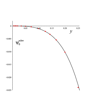
Figure 1: The behavior of the regularized scalar field (26) in the Schwarzschild case ($w=0$) as a function of $y$ is shown in comparison with existing numerical values. The data points are taken from Table I of Ref. DiazRivera:2004ik .

IV Scalar self-force

The scalar self-force is given by

$$F_{\alpha}(x^{\mu}) = q\nabla_{\alpha}\psi(x^{\mu})$$ (31)

$$= -q\nabla_{\alpha}\sum_{lm}G_{lm\omega}(r,r_{0})\Big{|}_{\omega=m\Omega}r_{0}q_{lm}e^{-im\Omega t}Y_{lm}(\theta,\phi)\,,$$

with nonvanishing components

$$F_{t\,(\pm)}^{0} = -\Omega F_{\phi\,(\pm)}^{0}=i\Omega\frac{4\pi q^{2}}{\Gamma}\sum_{lm}m\,G_{lm\omega}(r,r_{0})\Big{|}_{r=r_{0}^{\pm},\,\omega=m\Omega}|Y_{lm}(\pi/2,0)|^{2}\,,$$

$$F_{r\,(\pm)}^{0} = -\frac{4\pi q^{2}}{\Gamma}\sum_{lm}\partial_{r}G_{lm\omega}(r,r_{0})\Big{|}_{r=r_{0}^{\pm},\,\omega=m\Omega}|Y_{lm}(\pi/2,0)|^{2}\,,$$ (32)

once evaluated at the position of the scalar charge, i.e., in the limit $r\to r_{0}^{\pm}$. After summing over $m$, the divergent behavior for large $l$ is removed by

$$F_{\alpha}^{0\,\rm reg}=\sum_{l}\left[\frac{1}{2}\left(F_{\alpha\,(+)}^{0l}+F_{\alpha\,(-)}^{0l}\right)-B_{\alpha}\right]\,,$$ (33)

where $F_{\alpha\,(\pm)}^{0l}$ denote the limits $r\to r_{0}^{\pm}$ of each mode and the $l$-independent quantities $B_{\alpha}$ are suitable regularization parameters. The subtraction term for the radial component turns out to be (in units of $q$)

$$B_{r} = -\frac{1}{2}y^{2}+\left(-\frac{1}{8}+\frac{1}{3}w\right)y^{3}+\left(-\frac{21}{128}+\frac{1}{2}w-\frac{7}{18}w^{2}\right)y^{4}+\left(-\frac{53}{512}+\frac{57}{64}w-\frac{2}{3}w^{2}+\frac{44}{81}w^{3}\right)y^{5}$$ (34)

$$+\left(\frac{12607}{32768}+\frac{97}{96}w-\frac{331}{384}w^{2}+w^{3}-\frac{5}{6}w^{4}\right)y^{6}$$

$$+\left(\frac{306759}{131072}-\frac{18433}{16384}w+\frac{4517}{2304}w^{2}+\frac{1055}{864}w^{3}-\frac{130}{81}w^{4}+\frac{988}{729}w^{5}\right)y^{7}+O(y^{8})\,,$$

whereas $B_{t}=0$.

The final result for the regularized temporal and radial components of the self force valid through 7.5PN order is (in units of $q$)

$$F_{t}^{0\,\rm reg} = \frac{1}{3}y^{4}+\left(-\frac{1}{6}+\frac{2}{9}w\right)y^{5}+\frac{2}{3}\pi y^{11/2}+\left(-\frac{77}{24}+\frac{23}{18}w-\frac{1}{9}w^{2}\right)y^{6}+\left(\frac{9}{5}+\frac{4}{9}w\right)\pi y^{13/2}$$

$$+\left[\frac{7721}{3600}-\frac{1753}{675}w+\frac{10}{27}w^{2}+\frac{28}{243}w^{3}+\frac{2}{3}(1-w)^{3/2}+\frac{4}{9}\pi^{2}+\left(-\frac{76}{45}+\frac{16}{45}w\right)\gamma+\left(-\frac{76}{45}+\frac{16}{45}w\right)\ln(2)\right.$$

$$\left.+\left(-\frac{38}{45}+\frac{8}{45}w\right)\ln(y)\right]y^{7}$$

$$+\left(-\frac{3761}{420}+\frac{27}{5}w-\frac{2}{9}w^{2}\right)\pi y^{15/2}+O(y^{8})\,,$$

$$F_{r}^{0\,\rm reg} = \left[-\frac{2}{9}+\left(\frac{7}{64}-\frac{1}{64}w\right)\pi^{2}-\frac{4}{3}\gamma-\frac{4}{3}\ln(2)-\frac{2}{3}\ln(y)\right]y^{5}$$ (35)

$$+\left[\frac{604}{45}-\frac{41}{27}w+\left(\frac{29}{1024}-\frac{239}{3072}w+\frac{1}{96}w^{2}\right)\pi^{2}-\left(\frac{14}{3}+\frac{4}{9}w\right)\gamma-\left(\frac{66}{5}+\frac{4}{9}w\right)\ln(2)-\left(\frac{7}{3}+\frac{2}{9}w\right)\ln(y)\right]y^{6}$$

$$+\left(-\frac{38}{45}+\frac{8}{45}w\right)\pi y^{13/2}$$

$$+\left[\frac{1511}{140}+\frac{473}{90}w+\frac{103}{81}w^{2}+\left(\frac{1335}{2048}-\frac{1}{16}w+\frac{151}{2304}w^{2}-\frac{7}{576}w^{3}\right)\pi^{2}+\left(\frac{31}{2}-\frac{28}{3}w+\frac{8}{27}w^{2}\right)\gamma\right.$$

$$\left.+\left(\frac{857}{14}-\frac{268}{15}w+\frac{8}{27}w^{2}\right)\ln(2)-\frac{2187}{70}\ln(3)+\left(\frac{31}{4}-\frac{14}{3}w+\frac{4}{27}w^{2}\right)\ln(y)\right]y^{7}$$

$$+\left(-\frac{139}{35}+\frac{2378}{4725}w+\frac{8}{135}w^{2}\right)\pi y^{15/2}+O(y^{8})\,,$$

respectively.

In the Schwarzschild limit ($w\to 0$) we have

$$F_{t}^{0\,\rm reg,\,schw} = \frac{1}{3}y^{4}-\frac{1}{6}y^{5}+\frac{2}{3}\pi y^{11/2}-\frac{77}{24}y^{6}+\frac{9}{5}\pi y^{13/2}$$

$$+\left[\frac{10121}{3600}+\frac{4}{9}\pi^{2}-\frac{76}{45}\gamma-\frac{76}{45}\ln(2)-\frac{38}{45}\ln(y)\right]y^{7}$$

$$-\frac{3761}{420}\pi y^{15/2}+O(y^{8})\,,$$

$$F_{r}^{0\,\rm reg,\,schw} = \left[-\frac{2}{9}+\frac{7}{64}\pi^{2}-\frac{4}{3}\gamma-\frac{4}{3}\ln(2)-\frac{2}{3}\ln(y)\right]y^{5}$$ (36)

$$+\left[\frac{604}{45}+\frac{29}{1024}\pi^{2}-\frac{14}{3}\gamma-\frac{66}{5}\ln(2)-\frac{7}{3}\ln(y)\right]y^{6}$$

$$-\frac{38}{45}\pi y^{13/2}$$

$$+\left[\frac{1511}{140}+\frac{1335}{2048}\pi^{2}+\frac{31}{2}\gamma+\frac{857}{14}\ln(2)-\frac{2187}{70}\ln(3)+\frac{31}{4}\ln(y)\right]y^{7}$$

$$-\frac{139}{35}\pi y^{15/2}+O(y^{8})\,.$$

The leading 3PN and 4PN terms of the previous expressions agree with those of Ref. Hikida:2004hs . Furthermore, the comparison with available numerical results of Ref. DiazRivera:2004ik ; Warburton:2010eq shows again a very good agreement (see Table 2 and Fig. 2, where we refer to the most recent work Warburton:2010eq ).

Table 2: Comparison between the analytical expressions (IV) for the regularized temporal and radial components of the self force (in units of $q$) in the Schwarzschild case ($w=0$) and the numerical values taken from Tables II and III of Ref. Warburton:2010eq . The 2nd and 3rd column display the values obtained by our analytical expressions, whereas the last two columns show the difference with the above mentioned numerical results.

$y$	$F_{t}^{0\,\rm schw}$	$F_{r}^{0\,\rm schw}$	$\Delta F_{t}^{0\,\rm schw}$	$\Delta F_{r}^{0\,\rm schw}$
1/6	$3.088678309\times 10^{-4}$	$2.069192430\times 10^{-4}$	$5.20\times 10^{-5}$	$-3.92\times 10^{-5}$
1/7	$1.621300383\times 10^{-4}$	$9.086682872\times 10^{-5}$	$1.46\times 10^{-5}$	$-1.24\times 10^{-5}$
1/8	$9.278324817\times 10^{-5}$	$4.535558187\times 10^{-5}$	$4.94\times 10^{-6}$	$-4.53\times 10^{-6}$
1/10	$3.667967766\times 10^{-5}$	$1.462629728\times 10^{-5}$	$8.23\times 10^{-7}$	$-8.42\times 10^{-7}$
1/14	$9.180183375\times 10^{-6}$	$2.785864322\times 10^{-6}$	$5.66\times 10^{-8}$	$-6.58\times 10^{-8}$
1/20	$2.148236416\times 10^{-6}$	$4.981418996\times 10^{-7}$	$3.36\times 10^{-9}$	$-4.35\times 10^{-9}$
1/30	$4.175425467\times 10^{-7}$	$7.191466709\times 10^{-8}$	$1.36\times 10^{-10}$	$-1.96\times 10^{-10}$
1/50	$5.359926673\times 10^{-8}$	$6.350626477\times 10^{-9}$	$2.40\times 10^{-12}$	$-3.93\times 10^{-12}$
1/70	$1.391199738\times 10^{-8}$	$1.284814550\times 10^{-9}$	$1.67\times 10^{-13}$	$-3.15\times 10^{-13}$
1/100	$3.335029050\times 10^{-9}$	$2.356682550\times 10^{-10}$	$9.90\times 10^{-15}$	$-6.83\times 10^{-14}$

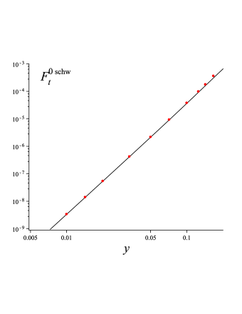
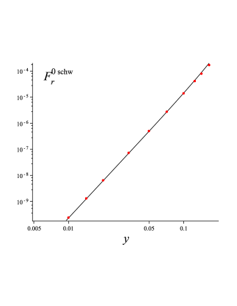
Figure 2: Comparison of numerical data from Ref. Warburton:2010eq for the regularized temporal and radial components of the self force (in units of $q$) in the Schwarzschild case ($w=0$) with the behavior of the corresponding analytical expressions (IV).

V Scalar radiation

Let us compute the amount of scalar radiation either flowing into the hole or transmitted at spatial infinity. We need to construct the solution to the non-homogeneous wave equation (10) which satisfies purely ingoing-wave boundary conditions at the black hole horizon and purely outgoing-wave boundary conditions at infinity. This is accomplished by using the two kinds of solutions $R^{H,\infty}_{lm\omega}$ to the corresponding homogeneous equation with asymptotic behavior Teukolsky:1973ha ; Press:1973zz ; Teukolsky:1974yv

$$R^{H}_{lm\omega} \to \left\{\begin{array}[]{ll}B^{\rm trans}e^{-i\omega r_{*}}\,,&r\to r_{+}\\[12.91663pt] B^{\rm ref}\displaystyle\frac{e^{i\omega r_{*}}}{r}+B^{\rm inc}\displaystyle\frac{e^{-i\omega r_{*}}}{r}\,,&r\to\infty\\ \end{array}\right.\,,$$ (39)

$$R^{\infty}_{lm\omega} \to \left\{\begin{array}[]{ll}C^{\rm up}e^{i\omega r_{*}}+C^{\rm ref}e^{-i\omega r_{*}}\,,&r\to r_{+}\\[12.91663pt] C^{\rm trans}\displaystyle\frac{e^{i\omega r_{*}}}{r}\,,&r\to\infty\\ \end{array}\right.\,,$$ (42)

where $r_{*}$ is the tortoise-like coordinate defined by ${dr_{*}}/{dr}={r^{2}}/{\Delta}$, i.e.,

$$r_{*}=r+\frac{2Mr_{+}}{r_{+}-r_{-}}\ln\frac{r-r_{+}}{2M}-\frac{2Mr_{-}}{r_{+}-r_{-}}\ln\frac{r-r_{-}}{2M}\,.$$ (43)

The final solution is given by Sasaki:2003xr

$$R_{lm\omega}(r)=Z^{H}_{lm\omega}(r)R^{\infty}_{lm\omega}(r)+Z^{\infty}_{lm\omega}(r)R^{H}_{lm\omega}(r)\,,$$ (44)

where

$$Z^{H}_{lm\omega}(r) = \frac{-1}{W_{lm\omega}}\int_{r_{+}}^{r}R^{H}_{lm\omega}(r^{\prime})\Delta(r^{\prime})S_{lm\omega}\delta(r^{\prime}-r_{0})dr^{\prime}\,,$$

$$Z^{\infty}_{lm\omega}(r) = \frac{-1}{W_{lm\omega}}\int_{r}^{\infty}R^{\infty}_{lm\omega}(r^{\prime})\Delta(r^{\prime})S_{lm\omega}\delta(r^{\prime}-r_{0})dr^{\prime}\,,$$

and $W_{lm\omega}=2i\omega C^{\rm trans}B^{\rm inc}$ is the constant Wronskian. The asymptotic behaviors of $R_{lm\omega}$ at the horizon and at infinity are then

$$R_{lm\omega}(r\to r_{+}) \to B^{\rm trans}Z^{\infty}_{lm\omega}(r_{+})e^{-i\omega r_{*}}\,,$$

$$R_{lm\omega}(r\to\infty) \to C^{\rm trans}Z^{H}_{lm\omega}(\infty)\frac{e^{i\omega r_{*}}}{r}\,,$$ (46)

respectively, so that one can define the amplitudes

$${\mathcal{Z}}^{H}_{lm\omega}=B^{\rm trans}Z^{\infty}_{lm\omega}(r_{+})\,,\qquad{\mathcal{Z}}^{\infty}_{lm\omega}=C^{\rm trans}Z^{H}_{lm\omega}(\infty)\,.$$ (47)

Explicitly we find

$${\mathcal{Z}}^{H}_{lm\omega} = 2\pi\frac{B^{\rm trans}}{W_{lm\omega}}\,r_{0}q_{lm\omega}R^{\infty}_{lm\omega}(r_{0})\delta(\omega-m\Omega)$$

$$\equiv 2\pi\tilde{\mathcal{Z}}^{H}_{lm}\delta(\omega-m\Omega)\,,$$

$${\mathcal{Z}}^{\infty}_{lm\omega} = 2\pi\frac{C^{\rm trans}}{W_{lm\omega}}\,r_{0}q_{lm\omega}R^{H}_{lm\omega}(r_{0})\delta(\omega-m\Omega)$$ (48)

$$\equiv 2\pi\tilde{\mathcal{Z}}^{\infty}_{lm}\delta(\omega-m\Omega)\,.$$

The energy flux at infinity is thus given by Teukolsky:1973ha ; Press:1973zz ; Teukolsky:1974yv

$$\frac{dE^{\infty}}{dt}=\sum_{lm}\frac{\omega^{2}}{4\pi}|\tilde{\mathcal{Z}}^{\infty}_{lm}|^{2}\,,$$ (49)

while the energy flux at the event horizon is

$$\frac{dE^{H}}{dt}=\sum_{lm}\frac{M\omega^{2}r_{+}}{2\pi}|\tilde{\mathcal{Z}}^{H}_{lm}|^{2}\,,$$ (50)

with $\tilde{\mathcal{Z}}^{H,\infty}_{lm}$ defined in Eq. (V) and $\omega=m\Omega$.

For the computation of the amplitudes and the transmission coefficients we have used the MST ingoing ad upgoing solutions, which satisfy the proper boundary conditions at the horizon and at infinity for any given value of $l$, i.e., $R^{H}_{lm\omega}(r)=R^{\rm in(MST)}_{lm\omega}(r)$ and $R^{\infty}_{lm\omega}(r)=R^{\rm up(MST)}_{lm\omega}(r)$. The corresponding transmission coefficients are given by Sasaki:2003xr

$$B^{\rm trans} = e^{i\frac{\kappa}{2}(\epsilon+\tau)\left(1+\frac{2\ln\kappa}{1+\kappa}\right)}\sum_{n=-\infty}^{\infty}a_{n}\,,$$

$$C^{\rm trans} = \omega^{-1}e^{i\epsilon\left(\ln\epsilon-\frac{1-\kappa}{2}\right)}A_{-}^{\nu}\,,$$ (51)

where

$$A_{-}^{\nu}=2^{-1+i\epsilon}e^{-\frac{\pi}{2}i(\nu+1)}e^{-\frac{\pi}{2}\epsilon}\sum_{n=-\infty}^{\infty}(-1)^{n}\frac{(\nu+1-i\epsilon)_{n}}{(\nu+1+i\epsilon)_{n}}\,a_{n}\,.$$ (52)

The definitions of the various quantities $\epsilon,\tau,\nu,a_{n}$ are given in Appendix A.2 for convenience.

We find (in units of $q$)

$$\frac{dE^{\infty}}{dt} = \left(\frac{dE^{\infty}}{dt}\right)_{N}\left\{1+\left(-2+\frac{2}{3}w\right)y+2\pi y^{3/2}+\left(-10+\frac{13}{3}w-\frac{1}{3}w^{2}\right)y^{2}+\left(\frac{12}{5}+\frac{4}{3}w\right)\pi y^{5/2}\right.$$

$$+\left[\frac{1331}{75}-\frac{2203}{225}w+\frac{4}{9}w^{2}+\frac{28}{81}w^{3}+\frac{4}{3}\pi^{2}\right.$$

$$\left.+\left(-\frac{76}{15}+\frac{16}{15}w\right)\gamma+\left(-\frac{76}{15}+\frac{16}{15}w\right)\ln(2)+\left(-\frac{38}{15}+\frac{8}{15}w\right)\ln(y)\right]y^{3}$$

$$\left.+\left(-\frac{521}{14}+\frac{86}{5}w-\frac{2}{3}w^{2}\right)\pi y^{7/2}+O(y^{4})\right\}\,,$$

$$\frac{dE^{H}}{dt} = \left(\frac{dE^{\infty}}{dt}\right)_{N}2(1-w)(1+\sqrt{1-w})\left\{y^{3}+\left(2-\frac{4}{3}w\right)y^{4}+\left(3-\frac{7}{3}w+2w^{2}\right)y^{5}\right.$$ (53)

$$+\left[\frac{1231}{75}-\frac{793}{225}w+\frac{32}{9}w^{2}-\frac{260}{81}w^{3}+\frac{1}{1-w}+\left(-\frac{38}{15}+\frac{8}{15}w\right)\ln(1-w)+\frac{1}{(1-w)^{1/2}}\left(\frac{4}{3}-\frac{2}{3}w\right)\pi^{2}\right.$$

$$\left.\left.-\frac{8}{3}\gamma+\left(-\frac{116}{15}+\frac{16}{15}w\right)\ln(2)+\left(-\frac{32}{5}+\frac{16}{15}w\right)\ln(y)\right]y^{6}\right.$$

$$\left.+\left[\frac{1769}{225}-\frac{46}{15}w+\frac{907}{675}w^{2}-\frac{473}{81}w^{3}+\frac{1309}{243}w^{4}+\frac{1}{1-w}\left(4-\frac{10}{3}w\right)+\left(-\frac{76}{15}+\frac{40}{9}w-\frac{32}{45}w^{2}\right)\ln(1-w)\right.\right.$$

$$\left.\left.+\frac{1}{(1-w)^{1/2}}\left(\frac{8}{3}-\frac{28}{9}w+\frac{8}{9}w^{2}\right)\pi^{2}+\left(\frac{64}{15}+\frac{8}{9}w\right)\gamma+\left(-\frac{88}{15}+\frac{88}{9}w-\frac{64}{45}w^{2}\right)\ln(2)\right.\right.$$

$$\left.\left.+\left(-8+\frac{28}{3}w-\frac{64}{45}w^{2}\right)\ln(y)\right]y^{7}\right.$$

$$\left.+\left(-\frac{56}{45}+\frac{16}{45}w\right)\pi y^{15/2}\right.$$

$$\left.+\left[-\frac{208762}{7875}+\frac{10034656}{165375}w-\frac{4518949}{165375}w^{2}+\frac{1162}{675}w^{3}+10w^{4}-\frac{28}{3}w^{5}+\frac{1}{1-w}\left(9-\frac{44}{3}w+\frac{25}{3}w^{2}\right)\right.\right.$$

$$\left.\left.+\left(-\frac{1818}{175}+\frac{17086}{1575}w-\frac{10804}{1575}w^{2}+\frac{16}{15}w^{3}\right)\ln(1-w)+\frac{1}{(1-w)^{1/2}}\left(\frac{36}{5}-\frac{446}{45}w+\frac{262}{45}w^{2}-\frac{4}{3}w^{3}\right)\pi^{2}\right.\right.$$

$$\left.\left.+\left(\frac{608}{105}-\frac{344}{45}w-\frac{8}{9}w^{2}\right)\gamma+\left(-\frac{1124}{75}+\frac{22132}{1575}w-\frac{23008}{1575}w^{2}+\frac{32}{15}w^{3}\right)\ln(2)\right.\right.$$

$$\left.\left.+\left(-\frac{9388}{525}+\frac{3128}{175}w-\frac{7436}{525}w^{2}+\frac{32}{15}w^{3}\right)\ln(y)\right]y^{8}\right.$$

$$\left.+\left(\frac{88}{225}+\frac{196}{675}w-\frac{16}{135}w^{2}\right)\pi y^{17/2}+O(y^{9})\right\}\,,$$

where

$$\left(\frac{dE^{\infty}}{dt}\right)_{N}=\frac{1}{3}y^{4}\,,$$ (54)

in terms of the gauge-invariant variable $y$ (see Eq. (24)). Note that the flux at infinity is computed up to the 3.5PN order, i.e., at $O(y^{7/2})$ included (see Appendix B). The leading contribution to the flux on the horizon, instead, enters at 3PN order beyond the lowest order, and is computed through $O(y^{17/2})$.

In the Schwarzschild case ($w\to 0$) the previous expressions reduce to

$$\frac{dE^{\infty}}{dt} = \left(\frac{dE^{\infty}}{dt}\right)_{N}\left[1-2y+2\pi y^{3/2}-10y^{2}+\frac{12}{5}\pi y^{5/2}+\left(\frac{1331}{75}+\frac{4}{3}\pi^{2}-\frac{76}{15}\gamma-\frac{76}{15}\ln(2)-\frac{38}{15}\ln(y)\right)y^{3}\right.$$

$$\left.-\frac{521}{14}\pi y^{7/2}+O(y^{4})\right]\,,$$

$$\frac{dE^{H}}{dt} = \left(\frac{dE^{\infty}}{dt}\right)_{N}4y^{3}\left[1+2y+3y^{2}+\left(\frac{1306}{75}+\frac{4}{3}\pi^{2}-\frac{8}{3}\gamma-\frac{116}{15}\ln(2)-\frac{32}{5}\ln(y)\right)y^{3}\right.$$ (55)

$$\left.+\left(\frac{2669}{225}+\frac{8}{3}\pi^{2}+\frac{64}{15}\gamma-\frac{88}{15}\ln(2)-8\ln(y)\right)y^{4}-\frac{56}{45}\pi y^{9/2}\right.$$

$$\left.+\left(-\frac{137887}{7875}+\frac{36}{5}\pi^{2}+\frac{608}{105}\gamma-\frac{1124}{75}\ln(2)-\frac{9388}{525}\ln(y)\right)y^{5}+\frac{88}{225}\pi y^{11/2}+O(y^{6})\right]\,,$$

whereas in the extreme RN case ($w\to 1$) we have

$$\frac{dE^{\infty}}{dt} = \left(\frac{dE^{\infty}}{dt}\right)_{N}\left[1-\frac{4}{3}y+2\pi y^{3/2}-6y^{2}+\frac{56}{15}\pi y^{5/2}+\left(\frac{3542}{405}+\frac{4}{3}\pi^{2}-4\gamma-4\ln(2)-2\ln(y)\right)y^{3}\right.$$

$$\left.-\frac{4343}{210}\pi y^{7/2}+O(y^{4})\right]\,,$$

$$\frac{dE^{H}}{dt} = \left(\frac{dE^{\infty}}{dt}\right)_{N}2y^{6}\left[1+\frac{2}{3}y+\frac{8}{3}y^{2}+O(y^{3})\right]\,.$$ (56)

Therefore, when the black hole is extremely charged the horizon-absorbed flux starts 3PN orders more beyond with respect to the non-extreme case.

Finally, we note that the angular momentum fluxes can be easily calculated through

$$\frac{dJ^{H,\infty}}{dt}=y^{-3/2}\frac{dE^{H,\infty}}{dt}\,.$$ (57)

Table 3: Comparison between the analytical expressions (V) for the energy fluxes at infinity and on the horizon (in units of $q$) in the Schwarzschild case ($w=0$) and the numerical values taken from Table I of Ref. Warburton:2010eq . The 2nd and 3rd column display the values of the flux radiated to infinity $\dot{E}^{\infty}$ and down to the horizon $\dot{E}^{H}$ (divided by the total flux $\dot{E}^{\rm tot}=\dot{E}^{\infty}+\dot{E}^{H}$), respectively, obtained by our analytical expressions, whereas the last two columns show the difference with the above mentioned numerical results.

$y$	$\dot{E}^{\infty}$	$\dot{E}^{H}/\dot{E}^{\rm tot}$	$\Delta\dot{E}^{\infty}$	$\Delta(\dot{E}^{H}/\dot{E}^{\rm tot})$
1/6	$2.096811267\times 10^{-4}$	$0.03565284588$	$4.55\times 10^{-5}$	$-4.85\times 10^{-3}$
1/8	$7.246350703\times 10^{-5}$	$0.01200009767$	$4.79\times 10^{-6}$	$-6.00\times 10^{-4}$
1/10	$3.052889221\times 10^{-5}$	$5.536219295\times 10^{-3}$	$8.48\times 10^{-7}$	$-1.36\times 10^{-4}$
1/20	$1.979588741\times 10^{-6}$	$5.854584422\times 10^{-4}$	$4.08\times 10^{-9}$	$1.45\times 10^{-5}$
1/40	$1.262462352\times 10^{-7}$	$6.785017170\times 10^{-5}$	$-1.95\times 10^{-11}$	$3.21\times 10^{-5}$

VI Concluding remarks

We have analyzed scalar self-force effects on a scalar charge moving along a circular orbit around a Reissner-Nordström black hole. The scalar wave equation is separated by using standard spherical harmonics (available here because of the underlying spherical symmetry of the background) and the field is decomposed into frequency modes. The associated radial equation is solved perturbatively in a PN framework by using the Green function method. The scalar field as well as the components of the self-force are then regularized at the particle’s position by subtracting the divergent term mode by mode, summing the infinite series up to a certain PN order. The MST approach has also been adopted for computing a number of radiative multipoles (up to $l=4$), so that our final result is accurate up to the 7.5PN order, i.e., up to the order $O(y^{15/2})$ included in terms of the dimensionless gauge-invariant frequency variable $y=(M\Omega)^{2/3}$. Since the scalar charge interacts only gravitationally with the background field, the coupling with the black hole electromagnetic charge is quadratic. The two limiting cases of a Schwarzschild black hole (which was missing in the literature and represents by itself an interesting byproduct of our work) and of an extreme Reissner-Nordström black hole are discussed explicitly. The comparison of the analytically computed regularized field and self-force components with existing results in the Schwarzschild case Detweiler:2002gi ; Warburton:2010eq has shown a good agreement, the difference between analytically and numerically produced values ranging from $\sim 10^{-14}$ in the weak-field region to $\sim 10^{-4}$ in the strong-field region.

We have also evaluated the radiation fluxes both at infinity and on the outer horizon up to $O(y^{7/2})$ and $O(y^{17/2})$ included, respectively. We have found that, when the black hole is extremely charged, the horizon-absorbed flux starts 3PN orders more beyond than the non-extreme case. The comparison with previous numerical results in the Schwarzschild case Warburton:2010eq has shown again a good agreement in both weak-field and strong-field regimes.

Appendix A Homogeneous solutions to the scalar wave equation

A.1 PN solutions

PN solutions have the form (III), i.e.,

$$R_{\rm in(PN)}^{lm\omega}(r) = r^{l}[1+A_{2}^{lm\omega}(r)\eta^{2}+A_{4}^{lm\omega}(r)\eta^{4}+A_{6}^{lm\omega}(r)\eta^{6}+A_{8}^{lm\omega}(r)\eta^{8}+\ldots]\,,$$

$$R_{\rm up(PN)}^{lm\omega}(r) = R_{\rm in(PN)}^{-l-1m\omega}(r)\,.$$ (58)

The first coefficients are given by

$$A_{2}^{lm\omega}(r) = -\frac{Ml}{r}-\frac{\omega^{2}r^{2}}{2(2l+3)}\,,$$

$$A_{4}^{lm\omega}(r) = \frac{M^{2}}{r^{2}}\frac{l(l-1)(2l-1-\kappa^{2})}{2(2l-1)}+M\omega^{2}r\frac{l^{2}-5l-10}{2(2l+3)(l+1)}+\frac{\omega^{4}r^{4}}{8(2l+3)(2l+5)}\,,$$

$$A_{6}^{lm\omega}(r) = -\frac{M^{3}}{r^{3}}\frac{l(l-1)(l-2)(2l-1-3\kappa^{2})}{6(2l-1)}-2M^{2}\omega^{2}\frac{[3(2l-1)(2l+3)+(3l^{2}+3l-2)\kappa^{2}][(2l+1)\ln(r/R)-1]}{(2l-1)(2l+3)(2l+1)^{2}}$$

$$-M\omega^{4}r^{3}\frac{3l^{3}-27l^{2}-142l-136}{24(l+1)(l+2)(2l+3)(2l+5)}-\frac{\omega^{6}r^{6}}{48(2l+3)(2l+5)(2l+7)}\,,$$

$$A_{8}^{lm\omega}(r) = \frac{M^{4}}{r^{4}}\frac{l(l-1)(l-2)(l-3)}{24(2l-1)(2l-3)}[(2l-1)(2l-3)-3\kappa^{2}(4l-6-\kappa^{2})]$$ (59)

$$+\frac{M^{3}\omega^{2}}{r}\left\{-\frac{4l^{6}-32l^{5}-99l^{4}-241l^{3}-436l^{2}-276l-36}{6l(2l+3)(2l+1)^{2}}+\frac{48l^{5}+348l^{4}+540l^{3}+126l^{2}-120l-36}{6l(2l+3)(2l-1)(2l+1)^{2}}\kappa^{2}\right.$$

$$\left.+\left[\frac{6l}{2l+1}+\frac{2l(3l^{2}+3l-2)}{(2l+3)(2l-1)(2l+1)}\kappa^{2}\right]\ln(r/R)\right\}$$

$$+M^{2}\omega^{2}r^{2}\left\{-\frac{24l^{7}+156l^{6}-1766l^{5}-13267l^{4}-29512l^{3}-23465l^{2}-2058l+2784}{48(l+1)(2l+3)^{2}(2l+5)(2l+1)^{2}(l+2)}\right.$$

$$+\frac{16l^{6}+80l^{5}-440l^{4}-2432l^{3}-2803l^{2}+11l+784}{16(2l-1)(2l+3)^{3}(2l+5)(2l+1)^{2}}\kappa^{2}$$

$$\left.+\left[\frac{3}{(2l+3)(2l+1)}+\frac{3l^{2}+3l-2}{(2l-1)(2l+3)^{2}(2l+1)}\kappa^{2}\right]\ln(r/R)\right\}$$

$$+M\omega^{6}r^{5}\frac{5l^{4}-60l^{3}-625l^{2}-1548l-1108}{240(l+3)(l+2)(2l+7)(2l+5)(2l+3)(l+1)}+\frac{\omega^{8}r^{8}}{384(2l+9)(2l+7)(2l+5)(2l+3)}\,,$$

where $R$ is a length scale. This solution, which we need however to compute the sum over all multipoles, becomes immediately inadequate, and one should use the MST technology. In fact, the coefficient $A_{4}$ of the “up” solution (obtained from $A_{4}^{lm\omega}(r)$ with $l\to-l-1$) diverges for $l=0$; similarly, higher order coefficients diverge for $l=1,2,\ldots$ etc.

A.2 MST solutions

The MST technique Mano:1996mf ; Mano:1996vt allows to find homogeneous solution to the radial equation which satisfy retarded boundary conditions at the horizon ($R_{\rm in(MST)}^{lm\omega}(r)$) and radiative boundary conditions at infinity ($R_{\rm up(MST)}^{lm\omega}(r)$).

The ingoing solution can be formally written as a convergent (at any finite value of $r$) series of hypergeometric functions

$$R_{\rm in(MST)}^{lm\omega}(x)=C_{\rm(in)}(x)\sum_{n=-\infty}^{\infty}a_{n}F(n+\nu+1-i\tau,-n-\nu-i\tau,1-i\epsilon-i\tau;x)\,,$$ (60)

with

$$C_{\rm(in)}(x)=e^{i\epsilon\kappa x}(-x)^{-i(\epsilon+\tau)/2}(1-x)^{i(\epsilon-\tau)/2}\,,$$ (61)

where the new variable $x=(r_{+}-r)/2M\kappa$ has been introduced and

$$\epsilon=2M\omega\,,\quad\tau=\frac{1}{2}\frac{\epsilon(\kappa^{2}+1)}{\kappa}\,.$$ (62)

The hypergeometric functions above are better evaluated by using the standard identity

$$F(a,b;c;x)=y^{a}\frac{\Gamma(c)\Gamma(b-a)}{\Gamma(b)\Gamma(c-a)}F(a,c-b,a-b+1;y)+y^{b}\frac{\Gamma(c)\Gamma(a-b)}{\Gamma(a)\Gamma(c-b)}F(b,c-a,b-a+1;y)\,,$$ (63)

involving the “small” variable $y=1/(1-x)$. Note that the overall factor $\Gamma(c)$ does not depend on $n$, so that it can be factored out.

The expansion coefficients $a_{n}$ satisfy the following three-term recurrence relation

$$\alpha_{n}^{\nu}a_{n+1}+\beta_{n}^{\nu}a_{n}+\gamma_{n}^{\nu}a_{n-1}=0\,,$$ (64)

where

$$\alpha_{n}^{\nu} = \frac{i\epsilon\kappa(n+\nu+1+i\epsilon)(n+\nu+1-i\epsilon)(n+\nu+1+i\tau)}{(n+\nu+1)(2n+2\nu+3)}\,,$$

$$\beta_{n}^{\nu} = -l(l+1)+(n+\nu)(n+\nu+1)+\epsilon\kappa\tau+\epsilon^{2}+\frac{\epsilon^{3}\kappa\tau}{(n+\nu)(n+\nu+1)}\,,$$

$$\gamma_{n}^{\nu} = -\frac{i\epsilon\kappa(n+\nu+i\epsilon)(n+\nu-i\tau)(n+\nu-i\epsilon)}{(n+\nu)(2n+2\nu-1)}\,.$$ (65)

Once the recurrence system has been solved for $n=1\ldots N$ and $n=-N\ldots-1$ for a given $N$ such that $a_{N}=0=a_{-N}$, the case $n=0$ with $a_{0}=1$ becomes a compatibility condition which yields the parameter

$$\nu=l+\sum_{k=1}^{\infty}\nu_{k}\epsilon^{2k}\,.$$ (66)

The solution of the recurrence system is rather involved (even in this relatively simple case). The structure of the expansion coefficients

$$a_{n}=\sum_{k=i}^{j}c_{nk}\epsilon^{k}$$ (67)

is summarized in Table 4 for $l=1$ and $N=15$, as an example.

Table 4: The structure of the expansion coefficients (67) of the recurrence relation is shown for $l=1$ and $N=15$, so that $a_{-15}=0=a_{15}$ and $a_{0}=1$.

$n$	$-14$	$-13$	$-12$	$-11$	$-10$	$-9$	$-8$	$-7$	$-6$	$-5$	$-4$	$-3$	$-2$	$-1$	$0$	$1$	$2$	$3$	$4$	$5$	$6$	$7$	$8$	$9$	$10$	$11$	$12$	$13$	$14$
$i$	$13$	$12$	$11$	$10$	$9$	$8$	$7$	$6$	$5$	$4$	$3$	$2$	$3$	$1$	-	$1$	$2$	$3$	$4$	$5$	$6$	$7$	$8$	$9$	$10$	$11$	$12$	$13$	$14$
$j$	$14$	$14$	$14$	$14$	$14$	$14$	$14$	$14$	$14$	$14$	$14$	$14$	$14$	$14$	-	$14$	$14$	$14$	$14$	$14$	$14$	$14$	$14$	$14$	$14$	$14$	$14$	$14$	$14$

The upgoing solution can be formally written as a convergent (at spatial infinity) series of irregular confluent hypergeometric functions with the same series coefficients

$$R_{\rm up(MST)}^{lm\omega}(z)=C_{\rm(up)}(z)\sum_{n=-\infty}^{\infty}a_{n}\frac{(\nu+1-i\epsilon)_{n}}{(\nu+1+i\epsilon)_{n}}\,(2iz)^{n}\Psi[n+\nu+1-i\epsilon,2n+2\nu+2;-2iz]\,,$$ (68)

with

$$C_{\rm(up)}(z)=(2z)^{\nu}e^{-\pi\epsilon}e^{-i\pi(\nu+1)}e^{iz}\left(1-\frac{\epsilon\kappa}{z}\right)^{-i(\epsilon+\tau)/2}\,,$$ (69)

where the new variable $z=\omega(r-r_{-})=\epsilon\kappa(1-x)$ has been introduced and $(A)_{n}=\Gamma(A+n)/\Gamma(A)$ is the Pochammer symbol. The irregular confluent hypergeometric functions above can be conveniently split into two pieces by using the identity

$$\Psi(a,b;\zeta)=\frac{\Gamma(1-b)}{\Gamma(a-b+1)}F(a,b;\zeta)+\zeta^{1-b}\frac{\Gamma(b-1)}{\Gamma(a)}F(a-b+1,2-b;\zeta)\,.$$ (70)

For instance, for $l=1$ we get

$$R_{\rm in(MST)}^{l=1}(r) = \frac{r}{M\kappa}-\frac{1}{\kappa}\left(1+\frac{\omega^{2}r^{3}}{10M}\right)\eta^{2}+\frac{i\omega r}{\kappa^{2}}\left[1+2\kappa+2\kappa^{2}-(1+\kappa)^{2}\gamma\right]\eta^{3}-\frac{\omega^{2}r^{2}}{\kappa}\left(\frac{7}{10}-\frac{\omega^{2}r^{3}}{280M}\right)\eta^{4}$$

$$-\frac{iM\omega}{\kappa^{2}}\left(1+\frac{\omega^{2}r^{3}}{10M}\right)\left[1+2\kappa+2\kappa^{2}-(1+\kappa)^{2}\gamma\right]\eta^{5}$$

$$-\left\{\left[\frac{16875+120375\kappa^{2}+87075\kappa^{4}+23790\kappa^{6}+1616\kappa^{8}}{75(15+4\kappa^{2})^{2}}+\left[1+2\kappa+2\kappa^{2}-(1+\kappa)^{2}\gamma\right]^{2}\right.\right.$$

$$\left.\left.-\frac{1}{6}(1+6\kappa^{2}+\kappa^{4})\pi^{2}-\frac{4}{15}\kappa^{2}(15+4\kappa^{2})\ln\left(\frac{2M\kappa\eta^{2}}{r}\right)\right]\frac{M\omega^{2}r}{2\kappa^{3}}-\frac{\omega^{4}r^{4}}{\kappa}\left(\frac{151}{2520}-\frac{\omega^{2}r^{3}}{15120M}\right)\right\}\eta^{6}$$

$$+O(\eta^{7})\,,$$

$$R_{\rm up(MST)}^{l=1}(r) = -\frac{i}{2\omega^{2}r^{2}}-\frac{i}{4}\left(1+\frac{4M}{\omega^{2}r^{3}}\right)\eta^{2}+\frac{M}{\omega r^{2}}\left(1+\frac{\omega^{2}r^{3}}{6M}-\gamma+i\pi\right)\eta^{3}-i\left(\frac{M}{r}-\frac{\omega^{2}r^{2}}{16}+\frac{3(5+\kappa^{2})M^{2}}{10\omega^{2}r^{4}}\right)\eta^{4}$$ (71)

$$+\left[\left(\frac{1}{3}-\frac{\gamma}{2}+\frac{i\pi}{2}\right)M\omega+\left(1-\gamma+i\pi\right)\frac{2M^{2}}{\omega r^{3}}-\frac{\omega^{3}r^{3}}{60}\right]\eta^{5}$$

$$+\left\{-\frac{2iM^{3}}{5\omega^{2}r^{5}}(5+3\kappa^{2})+\frac{iM^{2}}{15r^{2}}\left[-(15+4\kappa^{2})\ln(2\omega r\eta)+15(\gamma-i\pi)^{2}-(45+4\kappa^{2})\gamma+30i\pi-\frac{5}{2}\pi^{2}\right.\right.$$

$$\left.\left.+\frac{101250+67800\kappa^{2}+15435\kappa^{4}+848\kappa^{6}}{10(15+4\kappa^{2})^{2}}\right]+\frac{iM\omega^{2}r}{3}\left(2\ln(2\omega r\eta)+\gamma-\frac{61}{24}\right)-\frac{i\omega^{4}r^{4}}{288}\right\}\eta^{6}$$

$$+O(\eta^{7})\,,$$

having rescaled the “in” solution by the constant factor $\Gamma(c)$, with

$$\nu=1-\left(\frac{1}{2}+\frac{2}{15}\kappa^{2}\right)\epsilon^{2}-\frac{496125+680400\kappa^{2}+135990\kappa^{4}+12688\kappa^{6}}{189000(15+4\kappa^{2})}\epsilon^{4}+O(\epsilon^{6})\,.$$ (72)

Appendix B Energy fluxes

Using the notation of Ref. Sasaki:2003xr , the energy fluxes (49) and (50) can be written as

$$\frac{dE^{\infty}}{dt} = \left(\frac{dE^{\infty}}{dt}\right)_{N}\sum_{l=1}^{\infty}\sum_{m=-l}^{l}\eta^{\infty}_{lm}\,,$$

$$\frac{dE^{H}}{dt} = \left(\frac{dE^{\infty}}{dt}\right)_{N}2(1-w)(1+\sqrt{1-w})y^{3}\sum_{l=1}^{\infty}\sum_{m=-l}^{l}\eta^{H}_{lm}\,,$$ (73)

with $\eta^{H,\infty}_{l-m}=\eta^{H,\infty}_{lm}$. For small values of the dimensionless angular velocity variable $y$ the expansion coefficients behave as $\eta^{\infty}_{lm}\sim y^{l-1}$ and $\eta^{H}_{lm}\sim y^{2(l-1)}$, for fixed values of $m$. Therefore, since we have used the MST solutions up to $l=4$, our calculations of the flux at infinity and on the horizon are accurate up to the order $O(y^{7/2})$ and $O(y^{15/2})$ beyond the lowest order, respectively. For example, for $l=1$ the first few terms of the expansion are given by

$$\eta^{\infty}_{11} = \frac{1}{2}+\left(-\frac{13}{5}+\frac{1}{3}w\right)y+\pi y^{3/2}+\left(\frac{1123}{350}+\frac{1}{30}w-\frac{1}{6}w^{2}\right)y^{2}+\left(-\frac{26}{5}+\frac{2}{3}w\right)\pi y^{5/2}$$

$$+\left[\frac{10958}{945}-\frac{12427}{3150}w+\frac{26}{45}w^{2}+\frac{14}{81}w^{3}+\frac{2}{3}\pi^{2}+\left(-\frac{38}{15}+\frac{8}{15}w\right)\gamma+\left(-\frac{38}{15}+\frac{8}{15}w\right)\ln(2)\right.$$

$$\left.+\left(-\frac{19}{15}+\frac{4}{15}w\right)\ln(y)\right]y^{3}+\left(\frac{1123}{175}+\frac{1}{15}w-\frac{1}{3}w^{2}\right)\pi y^{7/2}+O(y^{4})\,,$$

$$\eta^{H}_{11} = \frac{1}{2}+\left(1-\frac{2}{3}w\right)y+\left(\frac{11}{10}-\frac{23}{30}w+w^{2}\right)y^{3}$$ (74)

$$+\left[\frac{971}{150}+\frac{347}{450}w+\frac{44}{45}w^{2}-\frac{130}{81}w^{3}+\frac{1}{2(1-w)}+\left(-\frac{19}{15}+\frac{4}{15}w\right)\ln(1-w)+\frac{1}{(1-w)^{1/2}}\left(\frac{2}{3}-\frac{1}{3}w\right)\pi^{2}\right.$$

$$\left.-\frac{4}{3}\gamma+\left(-\frac{58}{15}+\frac{8}{15}w\right)\ln(2)+\left(-\frac{16}{5}+\frac{8}{15}w\right)\ln(y)\right]y^{4}+O(y^{5})\,.$$

References

(1)
L. Barack,
“Gravitational self force in extreme mass-ratio inspirals,”
Class. Quant. Grav. 26, 213001 (2009)
[arXiv:0908.1664 [gr-qc]].
(2)
Y. Mino, M. Sasaki and T. Tanaka,
“Gravitational radiation reaction to a particle motion,”
Phys. Rev. D 55, 3457 (1997)
[gr-qc/9606018].
(3)
T. C. Quinn and R. M. Wald,
“An Axiomatic approach to electromagnetic and gravitational radiation reaction of particles in curved space-time,”
Phys. Rev. D 56, 3381 (1997)
[gr-qc/9610053].
(4)
T. C. Quinn,
“Axiomatic approach to radiation reaction of scalar point particles in curved space-time,”
Phys. Rev. D 62, 064029 (2000)
[gr-qc/0005030].
(5)
L. Barack, Y. Mino, H. Nakano, A. Ori and M. Sasaki,
“Calculating the gravitational selfforce in Schwarzschild space-time,”
Phys. Rev. Lett. 88, 091101 (2002)
[gr-qc/0111001].
(6)
L. Barack and A. Ori,
“Gravitational selfforce and gauge transformations,”
Phys. Rev. D 64, 124003 (2001)
[gr-qc/0107056].
(7)
S. L. Detweiler and B. F. Whiting,
“Self-force via a Green’s function decomposition,”
Phys. Rev. D 67, 024025 (2003)
[gr-qc/0202086].
(8)
E. Poisson,
“The Motion of point particles in curved space-time,”
Living Rev. Rel. 7, 6 (2004)
[gr-qc/0306052].
(9)
L. M. Burko,
“Self-force on static charges in Schwarzschild space-time,”
Class. Quant. Grav. 17, 227 (2000)
[gr-qc/9911042].
(10)
L. Barack,
“Self-force on a scalar particle in spherically symmetric space-time via mode sum regularization: Radial trajectories,”
Phys. Rev. D 62, 084027 (2000)
[gr-qc/0005042].
(11)
L. M. Burko,
“Self-force on particle in orbit around a black hole,”
Phys. Rev. Lett. 84, 4529 (2000)
[gr-qc/0003074].
(12)
A. G. Wiseman,
“The Self-force on a static scalar test charge outside a Schwarzschild black hole,”
Phys. Rev. D 61, 084014 (2000)
[gr-qc/0001025].
(13)
H. Nakano, Y. Mino and M. Sasaki,
“Self-force on a scalar charge in circular orbit around a Schwarzschild black hole,”
Prog. Theor. Phys. 106, 339 (2001)
[gr-qc/0104012].
(14)
L. M. Burko and Y. T. Liu,
“Self-force on a scalar charge in the space-time of a stationary, axisymmetric black hole,”
Phys. Rev. D 64, 024006 (2001)
[gr-qc/0103008].
(15)
L. Barack and A. Ori,
“Regularization parameters for the self-force in Schwarzschild space-time. 1. Scalar case,”
Phys. Rev. D 66, 084022 (2002)
[gr-qc/0204093].
(16)
S. L. Detweiler, E. Messaritaki and B. F. Whiting,
“Self-force of a scalar field for circular orbits about a Schwarzschild black hole,”
Phys. Rev. D 67, 104016 (2003)
[gr-qc/0205079].
(17)
H. Nakano, N. Sago and M. Sasaki,
“Gauge problem in the gravitational self-force. 2. First post-Newtonian force under Regge-Wheeler gauge,”
Phys. Rev. D 68, 124003 (2003)
[gr-qc/0308027].
(18)
W. Hikida, S. Jhingan, H. Nakano, N. Sago, M. Sasaki and T. Tanaka,
“A New analytical method for self-force regularization. 1. Scalar charged particle in Schwarzschild space-time,”
Prog. Theor. Phys. 111, 821 (2004)
[gr-qc/0308068].
(19)
L. M. Diaz-Rivera, E. Messaritaki, B. F. Whiting and S. L. Detweiler,