Modeling dark matter subhalos in a constrained galaxy:
Global mass and boosted annihilation profiles

Abstract

The interaction properties of cold dark matter (CDM) particle candidates, such as those of weakly interacting massive particles (WIMPs), generically lead to the structuring of dark matter on scales much smaller than typical galaxies, potentially down to $\sim 10^{-10}M_{\odot}$. This clustering translates into a very large population of subhalos in galaxies and affects the predictions for direct and indirect dark matter searches (gamma rays and antimatter cosmic rays). In this paper, we elaborate on previous analytic works to model the Galactic subhalo population, while remaining consistent with current observational dynamical constraints on the Milky Way. In particular, we propose a self-consistent method to account for tidal effects induced by both dark matter and baryons. Our model does not strongly rely on cosmological simulations, as they can hardly be fully matched to the real Milky Way, apart from setting the initial subhalo mass fraction. Still, it allows us to recover the main qualitative features of simulated systems. It can further be easily adapted to any change in the dynamical constraints, and can be used to make predictions or derive constraints on dark matter candidates from indirect or direct searches. We compute the annihilation boost factor, including the subhalo-halo cross product. We confirm that tidal effects induced by the baryonic components of the Galaxy play a very important role, resulting in a local average subhalo mass density $\lesssim 1\%$ of the total local dark matter mass density, while selecting the most concentrated objects and leading to interesting features in the overall annihilation profile in the case of a sharp subhalo mass function. Values of global annihilation boost factors range from $\sim 2$ to $\sim 20$, while the local annihilation rate is about half as much boosted.

I Introduction

While the long-standing issue of the origin of dark matter (DM) is still pending, many experiments involved in this quest have recently reached the sensitivity to probe the relevant parameter space for one of the most popular particle candidates, the WIMP, which finds specific realizations in many particle physics scenarios beyond the standard model (e.g. Refs. Primack et al. (1988); Jungman et al. (1996); Bergström (2000)). Among different search strategies, indirect DM searches (e.g. Refs. Carr et al. (2006); Porter et al. (2011); Lavalle and Salati (2012); Strigari (2013)) are becoming quite constraining for WIMPs annihilating through s-waves. This is particularly striking not only for indirect searches in gamma rays (e.g. Refs. Gunn et al. (1978); Bergström and Snellman (1988); Conrad et al. (2015)), but also in the antimatter cosmic-ray spectrum Silk and Srednicki (1984), both with positrons (e.g. Ref. Bergström et al. (2013)) and with antiprotons (e.g. Ref. Giesen et al. (2015)). For indirect searches, the way the Galactic dark matter halo is modeled is a fundamental piece in deriving constraints or testing detectability. For direct DM searches, whether the local DM density is smooth or may contain inhomogeneities also has important consequences (see e.g. Ref. Freese et al. (2013)).

A generic cosmological consequence of the WIMP scenario (among other CDM candidates) is the clustering of dark matter on very small, subgalactic scales, when the Universe enters the matter-domination era (e.g. Refs. Peebles (1984); Silk and Stebbins (1993); Kolb and Tkachev (1994); Chen et al. (2001); Hofmann et al. (2001); Berezinsky et al. (2003); Green et al. (2004); Loeb and Zaldarriaga (2005); Boehm and Schaeffer (2005); Profumo et al. (2006); Bertschinger (2006); Bringmann and Hofmann (2007); Visinelli and Gondolo (2015), and Ref. Bringmann (2009) for a review). Both analytic calculations (see a review in e.g. Ref. Berezinsky et al. (2014)) and cosmological simulations (e.g. Refs. Diemand et al. (2005, 2007a); Springel et al. (2008); Anderhalden and Diemand (2013); Ishiyama (2014)) show that many of these subhalos survive in galaxies against tidal disruption, and further constrain their properties. Consequently, the DM halo embedding the MW, if it is made of WIMPs, is not a smooth distribution of DM, but instead exhibits inhomogeneities in the form of many subhalos or their debris. In the context of self-annihilating DM candidates, this leads to the interesting consequence of enhancing the average annihilation rate with respect to the smooth-halo assumption Silk and Stebbins (1993). Generic methods to account for a subhalo population in the DM annihilation signal predictions were originally presented in Refs. Bergström et al. (1999); Ullio et al. (2002) for gamma rays, and in Refs. Lavalle et al. (2007, 2008) for antimatter cosmic rays.

While subhalos are now very often included when deriving constraints from the Galactic or extragalactic diffuse gamma-ray emissions (see e.g. Refs. Ullio et al. (2002); Pieri et al. (2011); Blanchet and Lavalle (2012); Serpico et al. (2012); Ajello et al. (2015), and a review in Ref. Fornasa and Sanchez-Conde (2015)), this is still barely the case for the antimatter channels (e.g. Refs. Giesen et al. (2015); Boudaud et al. (2015a)). In the latter case, although it was shown that subhalos could not enhance the predictions by orders of magnitude Lavalle et al. (2008); Pieri et al. (2011), the precision achieved by current experiments (see e.g. Refs. Adriani et al. (2009, 2010, 2014); Aguilar et al. (2016) for antiproton measurements) implies that even small changes in the predicted fluxes could still have a strong impact on constraints on the WIMP mass. In this paper, our aim is to provide a dynamically self-consistent model of a Galactic subhalo component in order to improve the constraints derived on s-wave annihilating WIMPs.

The paper develops as follows: A short overview of our method is presented in Sect. II, where the main steps are made clear. The instrumental part of our study is described in Sect. III, where we introduce the dark halo setup including both a smooth and a subhalo component, and where we discuss the tidal effects induced by both baryons and dark matter. We then discuss the mass profiles, the dark matter annihilation profile, and the corresponding differential and integrated annihilation boost factors in Sect. IV, which can be used in indirect detection studies. In that part, we also quantify the theoretical uncertainties coming from using different Galactic mass models, different tidal cutoff criteria, or other subhalo population properties. We conclude and present our perspectives in Sect. V.

II Overview of the model

We summarize below the main steps of the procedure we have developed in this study to get both a smooth Galactic halo and its subhalo population consistent with dynamical constraints:

• Select a complete and constrained Milky Way mass model that includes baryons (disk, bulge, etc.) and a DM halo, and which provides a good fit to kinematic data.

• Assume that the DM halo is separable in terms of a smooth component and a subhalo components which should be true from the initial stage of the Galactic halo formation to its currently observed state [see Sect. III.1 and Eq. (2)] – during the evolution of the halo, part of the subhalo component mass is stripped away by tidal effects and will be considered as fully transferred to the smooth component. Assume that equilibrium has been reached today.

• Assign a phase space to the subhalo component: each subhalo is considered to be an independent object characterized by (i) its initial mass (in a homogeneous background density), (ii) its concentration, and (iii) its position in the Milky Way (spherical orbits assumed) – associated distribution functions are initially independent (factorizable), but will become intricate (non-factorizable) as gravitational tidal effects come into play [see Sect. III.2.2 and item 5 below].

• Assume that the concentration and mass functions are initially the cosmological ones, i.e. position-independent [see Sect. III.3.1 and Sect. III.3.2]. Further assume that both the smooth and the subhalo components were initially following the same spatial distribution, which sets the initial spatial distribution for subhalos before tidal stripping and potential subsequent disruption [see Sect. III.3.3].

• Normalize the whole subhalo mass (or the total number of subhalos) from preferred prescriptions [this can be done from observational or structure formation constraints; before or after plugging tidal stripping, i.e. after item 6a or 6b below; see Sect. III.2.3].

• Determine how gravitational tides due to both the baryonic components and the whole dark matter content affect subhalos as a function of their properties (location, mass, and concentration), which allows to get the final phase-space distribution for subhalos [Sect. III.4 on tidal effects, which is a crucial part in this work]. In practice, we proceed by:

  • calculating the global tidal stripping induced by the host halo, which sets a first tidal radius $r_{t}$ [see Sect. III.4.1];

  • calculating the tidal stripping induced by disk shocking, which may reduce the tidal radius initially set by global halo tides [strong reduction in the central parts of the Galaxy, see Sect. III.4.2];

  • determining a criterion for disrupting subhalos depending on their tidal radii – so-called tidal disruption efficiency $\varepsilon_{t}$ [see Sect. III.4.4].

  The obtained final intricate phase-space function is mostly determined by the new concentration function, which has become spatial-dependent as a result of tidal disruption. This implies that the mass function also becomes spatial-dependent since integrated over concentration, and the initial spatial distribution gets modified, since integrated over mass. This final phase-space distribution should provide a more realistic description of subhalos, including tidal stripping and disruption inferred from all components of the constrained Galactic mass model, and therefore consistent with dynamical constraints by construction [see again Sect. III.2.2 for the description of the intricate phase space]. It is encoded in Eqs. (11) and (12) which, together with Eq. (2), define our constrained global DM halo model.

• Use this final subhalo distribution to get the smooth component from the overall constrained halo profile [see Eq. (2)], and to further compute observables relevant to DM searches [e.g. local density of subhalos, annihilation boost factor, etc. – see Sect. IV].

Not only this theoretical modeling allows to recover the main qualitative results obtained in zoomed cosmological simulations (e.g. the fact that the whole subhalo distribution is strongly depleted in the central regions of the Galaxy, while it dominates the mass profile in the outskirts), but it also allows to get a complete DM halo (including a smooth component and a subhalo component) which is fully consistent with current dynamical constraints. The latter point can actually hardly be achieved when directly importing results from cosmological simulations. Indeed, the dark and baryonic profiles found in Milky Way-like simulations, even if somewhat similar, can barely be fully matched to the detailed observed properties of the Milky Way, which are strongly constrained by kinematic data. Since these detailed properties play a central role in terms of tidal stripping, blindly extrapolating results from cosmological simulations will likely be plagued by inconsistencies, which we remedy here in a theoretically consistent, reproducible, and tuneable way. Instead, simulations remain instrumental to get insight on the physical processes themselves.

III The Milky Way dark halo and its subhalo population

In this section, we propose a self-consistent method to constrain the subhalo population of the MW dark halo and to derive therein the DM annihilation rate including all components. This method subscribes to two main principles: (i) accounting for existing dynamical constraints in the MW; (ii) starting from general assumptions, then comparing to and calibrating on high-resolution cosmological simulations only a posteriori.

In the following, any halo mass $m$ will, unless specified otherwise, express the mass contained within a sphere of radius $r_{200}$ such that

$$m=m(r_{200})=m_{200}=\frac{4\,\pi}{3}\,(200\times\rho_{c})\,r_{200}^{3}\,,$$ (1)

where $\rho_{c}$ is the critical density of the Universe as measured today, which we compute from the best-fit Hubble parameter obtained by the Planck Collaboration (combined analysis): $H_{0}=67.74$ km/s/Mpc.

III.1 Dark halo model

The most basic and obvious assumption one can make about the DM distribution in the Galaxy is that the DM density profile $\rho_{\rm tot}$ can be split into two components: one smooth, $\rho_{\rm sm}$, and another made of subhalos, $\rho_{\rm sub}$, such that at any position $\vec{x}$,

$$\rho_{\rm tot}(\vec{x})=\rho_{\rm sm}(\vec{x})+\rho_{\rm sub}(\vec{x})\,,$$ (2)

such that the total dark mass is given by

$$M_{200}=\int_{V_{200}}dV\,\rho_{\rm tot}(\vec{x})\,,$$ (3)

where $V_{200}$ is the spherical volume delineated by the associated pseudovirial radius $R_{200}$.

Furthermore, to get reliable predictions for DM annihilation signals, it is important to account for existing dynamical constraints on the DM profile. There have been significant efforts to improve Milky Way mass models in the recent years (e.g. Refs. Catena and Ullio (2010); Salucci et al. (2010); McMillan (2011); Bovy and Tremaine (2012); Bovy and Rix (2013); Piffl et al. (2014); Kafle et al. (2014); Bienaymé et al. (2014); McKee et al. (2015); Xia et al. (2016); Huang et al. (2016)), such that the dark halo is actually strongly constrained in its shape and related parameters. Modeling a clumpy dark halo in the context of DM searches can therefore strongly benefit from these results, and in any case should account for existing dynamical constraints. We stress that global dynamical studies like those cited above provide constraints on $\rho_{\rm tot}$, but not on $\rho_{\rm sm}$ and $\rho_{\rm sub}$ separately.

In many Galactic DM search studies involving subhalos, one usually exploits the results of high-resolution cosmological simulations either by putting a virtual observer at 8 kpc from the center of the simulated halo (irrespective of the differences between the real and simulated galaxy) and computing relevant observables, by rescaling simulation profiles to match with the measured local DM density, or by adding simulation-inspired fits of subhalo number density profiles to get predictions. However, as we will show later, tidal effects have a strong dependence on the details of the (baryonic and dark) matter content of the Milky Way. Therefore, since the Milky Way halo and its baryonic content are now rather strongly constrained, such blind matchings or extrapolations are likely to provide uncontrolled, or at least inconsistent, results (even if dubbed Milky Way-like, a cosmological simulation can hardly be fully matched to the Milky Way – e.g. the detailed halo profile and its parameters; the precise size, width, mass of the disk; intrinsic mass resolution limit; etc. – but to some extent). This motivates us to go beyond these simplistic recipes and propose a new approach. We still emphasize that cosmological simulations do provide very important and useful information about the subhalo dynamics, and we will take advantage of the generic subhalo properties inferred from simulations rather than the peculiar description of a single simulated clumpy halo, even though the latter case provides a very nice environment to study dynamical correlations between various galactic components or more specific physical processes.

From cosmological structure formation (see e.g. Refs. Cooray and Sheth (2002); Zentner (2007); Knobel (2012)), we know that galactic halos form rather late ($z\sim 6$) with respect to the smallest-scale halos expected in the WIMP scenario ($z\sim 80$). It is therefore reasonable to assume that the smooth and subhalo components follow the same spatial distribution when the Galactic halo forms. Then, as the Galaxy evolves, several changes occur: (i) further subhalos are accreted; and (ii) subhalos may experience mergers, stellar encounters, and tidal disruptions. Since the former phenomenon also concerns the smooth component, it should not modify the overall picture (subhalos may be considered as test particles among others). However, the latter must be taken into account, since it will reduce the subhalo number density in regions close to the terrestrial observers. This approximate trend is actually what is found in very high-resolution cosmological simulations, where the subhalo number density is shown to depart from the overall DM distribution essentially in the central regions of galaxies Diemand et al. (2008); Springel et al. (2008); Zhu et al. (2016). In the same references, the global DM profile (including subhalos) is found to be consistent with the seminal earlier results obtained by Navarro, Frenk, and White Navarro et al. (1996) (hereafter NFW) and subsequent refinements (e.g. Refs. Navarro et al. (2004); Merritt et al. (2006); Diemand et al. (2008); Navarro et al. (2010); Zhu et al. (2016)). Inner cored profiles can also be found as a result of efficient feedback originating in star formation and supernova explosions Macciò et al. (2012); Mollitor et al. (2015).

All this suggests the following method to try to build a self-consistent dark halo with a substructure component: (i) assume a global DM halo profile $\rho_{\rm tot}$ constrained by dynamical studies; (ii) start with a subhalo population tracking the smooth halo, such that both $\rho_{\rm sub}\propto\rho_{\rm tot}$ and $\rho_{\rm sm}\propto\rho_{\rm tot}$; (iii) plug in tidal disruption such that the mass contained in disrupted subhalos and in the pruned part of the survivors is transferred to the smooth-halo component; (iii) compare/cross-calibrate the final result with/onto high-resolution cosmological simulations. Before we translate this method in terms of equations for DM searches, we need to figure out how to express the mass density profile $\rho_{\rm sub}$ associated with subhalos. In practice, the smooth DM component will merely be determined from Eq. (2) as $\rho_{\rm sm}=\rho_{\rm tot}-\rho_{\rm sub}$, after having set $\rho_{\rm sub}$.

III.2 Accounting for dynamical constraints

As a template and dynamically constrained global dark halo, we will use the best-fit MW mass model obtained by McMillan McMillan (2011) (M11 hereafter), which turns out to be fully consistent with more recent studies (e.g. Refs. Piffl et al. (2014); Kafle et al. (2014); McMillan (2016)) while rather simple to implement. This model was derived from a Bayesian analysis run upon several observational data sets, photometric as well as kinematic, restricting to the terminal velocity curves measured for longitudes $|l|>45^{\circ}$ — this model does not address the complex structure of the very central regions of the MW, nor does it include any atomic or molecular gas component (we will use mass models including gas components in Sect. IV.4).

III.2.1 Global dark halo and baryons

M11 assumes a spherically symmetric NFW profile, given in terms of the general $\alpha\beta\gamma$ parametrization Hernquist (1990); Zhao (1996) as

$$\rho_{\rm tot}(r)=\rho_{\alpha\beta\gamma}(r)\equiv\rho_{s}\,\left(r/r_{s}\right)^{-\gamma}\,\left\{1+\left(r/r_{s}\right)^{\alpha}\right\}^{-\frac{(\beta-\gamma)}{\alpha}}\,,$$

(4)

with $(\alpha,\beta,\gamma)=(1,3,1)$ for an NFW profile. The M11 best-fit values for the scale density $\rho_{s}$ and the scale radius $r_{s}$ are given in Tab. 1. For the sake of comparison, we also introduce the Einasto dark matter profile Einasto (1965); Navarro et al. (2004):

$$\rho_{\rm ein}(r)=\rho_{s}\,\exp\left\{-\frac{2}{\alpha_{e}}\left[\left(\frac{r}{r_{s}}\right)^{\alpha_{e}}-1\right]\right\}\,.$$ (5)

This profile halo was used in a dynamical study complementary to and consistent with M11, presented in Ref. Catena and Ullio (2010) (CU10 hereafter). The associated parameters are also given in Tab. 1. Irrespective of the MW mass model, these dark matter profiles will also be used to describe the inner density profiles of subhalos (before tidal stripping). In the following, we will use M11 as our reference case.

Since we also aim at considering the baryonic components when dealing with tidal effects (see Ref. Bland-Hawthorn and Gerhard (2016) for a recent review), we provide the axisymmetric M11 bulge-disk density model below (with the convention $r^{2}=R^{2}+z^{2}$), where the subscript $b$ refers to the bulge and $d$ to the disk:

$$\rho_{b}(R,z) = \frac{\rho_{b}}{(1+r^{\prime}/r_{b})^{\alpha_{b}}}\,\exp\left\{-\left(\frac{r^{\prime}}{r_{b}^{c}}\right)^{2}\right\}\;,$$

$$\rho_{d}(R,z) = \frac{\Sigma_{d}}{2\,z_{d}}\,\exp\left\{-\frac{R}{R_{d}}-\frac{|z|}{z_{d}}\right\}\;,$$ (6)

where $r^{\prime}\equiv\sqrt{R^{2}+(z/q)^{2})}$, $q$ is the axial ratio, $\Sigma_{d}$ is the disk surface density, and the other parameters are scale parameters. All parameters are given in Tab. 2, where a two-component disk is explicit (thin and thick disks) – note that the above disk parameterization can also be relevant to additional gas components (see Sect. IV.4). Since the model was not fitted against observational data featuring the central regions of the Galaxy, the bulge parameters but $\rho_{b}$ are actually fixed to those obtained in Ref. Bissantz and Gerhard (2002). Note that such a disk profile can also be relevant to describing gaseous components, which have not been included in M11.

It will prove useful to have a spherical approximation of the disk density when dealing with global tides (see Sect. III.4.1). We readily derive it by demanding that the disk mass inside a sphere of radius $r$ equal the actual disk mass inside an infinite cylinder of radius $R$. It reads

$$\rho_{d,{\rm sph}}(r) = \frac{\Sigma_{d}}{2\,r}\,\exp\left\{-\frac{r}{R_{d}}\right\}\;.$$ (7)

One may find similar expressions with $R_{d}\leftrightarrow\sqrt{R_{d}^{2}+z_{d}^{2}}$ (e.g. Ref. Binney and Tremaine (2008)), but using one or another has absolutely no impact in this study.

MW mass model	Profile	$r_{200}$	$M_{200}$	$r_{s}$	$\rho_{s}$	$R_{\odot}$	$\rho_{\odot}$
		[kpc]	[$M_{\odot}$]	[kpc]	[GeV/cm3]	[kpc]	[GeV/cm3]
M11	NFW	237	$1.43\times 10^{12}$	20.2	0.32	8.29	0.395
CU10	Einasto($\alpha_{e}=0.22$)	208	$9.6\times 10^{11}$	16.07	0.11	8.25	0.386
M16	NFW	230.5	$1.31\times 10^{12}$	19.6	0.32	8.21	0.383

Table 1: Dark matter halo parameters for different Galactic mass models (best-fit models of Refs. McMillan (2011) [M11], Catena and Ullio (2010) [CU10], and McMillan (2016) [M16]).

MW mass model	$q$	$\alpha_{b}$	$r_{b}$	$r_{b}^{c}$	$\rho_{b}$	$R_{d}$ [kpc]	$z_{d}$ [kpc]	$\Sigma_{d}$ [$M_{\odot}/{\rm pc}^{2}$]
			[kpc]	[kpc]	[$M_{\odot}/{\rm pc}^{3}$]	(thin/thick)(HI/HII)	(thin/thick)(HI/HII)	(thin/thick)(HI/HII)
M11	0.5	1.8	0.075	2.1	95.6	(2.9/3.31)(-/-)	(0.3/0.9)(-/-)	(816.6/209.5)(-/-)
CU10	0.6	1.85	0.3879	0.872	1.37	(2.45/-)(7/1.5)†	(0.34/-)(0.085/0.045)†	(1154.12/-)(53.1/2180)†
M16	0.5	1.8	0.075	2.1	98.4	(2.5/3.02)(7/1.5)	(0.3/0.9)(0.085/0.045)	(896/183)(53.1/2180)

Table 2: Baryonic component parameters for different Galactic mass models (best-fit models of Refs. McMillan (2011) [M11], Catena and Ullio (2010) [CU10], and McMillan (2016) [M16]). ^†: The CU10 HI and HII gas disks are inferred from old data points, so we adopt the same parameterization as in M16 for simplicity – this has negligible impact on the final results.

III.2.2 The overall subhalo component

The very presence of subhalos in the Galactic host halo leads to strong DM inhomogeneities, so defining a global regular mass density function for subhalos implicitly implies averaging over a certain volume. In the following, we will assume that the whole Galaxy has reached an equilibrium state (no time dependence), and that subhalos are independent objects described over a phase space $w^{n}$ that includes their position $\vec{x}$, mass $m$, and concentration $c$ (we define these parameters in Sect. III.3). We also assume that a subhalo at position $\vec{x}$ can be described as an individual object lying in a local background density $\rho_{\rm tot}(\vec{x})$ constant over the size of the subhalo (coarse-grain approximation). With these assumptions, the subhalo phase-space number density reads

$$\frac{d^{n}N}{dw^{n}} = \frac{N_{\rm sub}}{K_{w}}\,\frac{d{\cal P}_{V}(\vec{x})}{dV}\,\frac{d{\cal P}_{m}(m)}{dm}\,\frac{d{\cal P}_{c}(c,m,\vec{x})}{dc}\;$$ (8)

$$= \frac{N_{\rm sub}}{K_{w}}\,\frac{d{\cal P}_{V,m,c}(\vec{x},m,c)}{dV\,dm\,dc}\,.$$

Without gravitational interactions between subhalos and the rest of the Milky Way, the phase space would be separable such that each ${\cal P}_{w}$ could be factorized. However, as we will see later, tidal effects induce non-trivial correlations between $\vec{x}$, $m$, and $c$, and the phase space becomes intricate. However, the individual ${\cal P}_{w}$s still define here effective “initial” conditions before tidal effects are plugged in, and are also necessary inputs to calculate the final local phase space (intricate concentration and mass functions at a given position $\vec{x}$). Parameter $K_{w}$ featured above is a normalization constant determined by the following closure relation:

$$\int dw^{n}\,\frac{d^{n}{\cal P}_{w}}{dw^{n}} = K_{w}$$

$$\Leftrightarrow\int dw^{n}\,\frac{d^{n}N}{dw^{n}} = N_{\rm sub}\;,$$ (9)

where $N_{\rm sub}$ is the total number of subhalos over the whole phase space embedded in the host dark halo. Each individual probability distribution function (PDF) $d{\cal P}_{w_{i}}/dw_{i}$, where $w=V,m,c$ ($V$ is the physical volume), is defined such that it is normalized over its phase-space subvolume $\delta W_{i}$ as

$$\int_{w_{i,{\rm min}}\in\delta W_{i}}^{w_{i,{\rm max}}\in\delta W_{i}}dw_{i}\,\frac{d{\cal P}_{w_{i}}}{dw_{i}}=1\,.$$ (10)

We emphasize that as long as these individual PDFs are uncorrelated (“initial” conditions), $K_{w}=1$, but this is generally not the case. In particular, tidal effects imply that each subhalo is actually featured by a tidal radius $r_{t}$ which depends on the initial subhalo mass $m$, its position $\vec{x}$ in the Galactic halo, and its concentration $c$ — we will detail the individual PDFs in Sect. III.3 and discuss the tidal disruption of subhalos in Sect. III.4. Therefore, tidal effects do induce an explicit correlation between the PDFs, making the subhalo phase space intricate and non-trivial, and leading here to $K_{w}\neq 1$. However, we can still self-consistently define the global subhalo number density $n_{\rm sub}$ profile as

$$\frac{dn_{\rm sub}(\vec{x},m)}{dm} = \frac{N_{\rm sub}}{K_{w}}\,\frac{d{\cal P}_{V}(\vec{x})}{dV}\,\frac{d{\cal P}_{m}(m)}{dm}\int_{c_{\rm min}(\vec{x})}^{c_{\rm max}}dc\,\frac{d{\cal P}_{c}}{dc}$$

$$\Longrightarrow\;\;n_{\rm sub}(\vec{x}) = \frac{N_{\rm sub}}{K_{w}}\,\frac{d{\cal P}_{V}(\vec{x})}{dV}\int_{m_{\rm min}}^{m_{\rm max}}dm\,\frac{d{\cal P}_{m}(m)}{dm}\int_{c_{\rm min}(\vec{x})}^{c_{\rm max}}dc\,\frac{d{\cal P}_{c}}{dc}\,,$$ (11)

where we wrote both the mass-differential form and its integral. The differential form is here expressed in terms of $m$, i.e. the initial (cosmological) subhalo mass contained inside an approximate virial radius assuming a homogeneous background matter, usually $r_{200}$, which is not the actual tidal subhalo mass $m_{t}$ (see Sect. III.3 for details) – we will show how to obtain the differential form in terms of $m_{t}$ in Sect. IV.2. It will also become clear in Sect. III.4.4 why tidal effects induce a spatial dependence of the minimal allowed concentration $c_{\rm min}(\vec{x})$, such that $n_{\rm sub}$ is actually very strongly depleted toward the central regions of the Galaxy in spite of the increase of $d{\cal P}_{V}/dV$.

We can also self-consistently define the global subhalo mass density profile as

$$\rho_{\rm sub}(\vec{x}) = N_{\rm sub}\,\widetilde{\langle m_{t}\rangle}(\vec{x})\,\frac{d{\cal P}_{V}(\vec{x})}{dV}\,,$$

$${\rm with}\;\widetilde{\langle m_{t}\rangle}(\vec{x}) \equiv \frac{1}{K_{w}}\,\int_{m_{\rm min}}^{m_{\rm max}}dm\,\frac{d{\cal P}_{m}}{dm}\int_{c_{\rm min}(\vec{x})}^{c_{\rm max}}dc\,\frac{d{\cal P}_{c}}{dc}\,m_{t}(r_{t}(c,m,\vec{x}),m,c)\;,$$ (12)

where $m_{t}$ is the tidal subhalo mass contained within the tidal radius $r_{t}$, to be contrasted again with $m$. The symbol $\widetilde{\langle\rangle}$ is not the average over the mass and concentration subpart of the phase space because of the normalization $K_{w}$, which is calculated over the full phase space. The real mean mass (or any other quantity depending on mass and concentration) is actually given by

$$\langle m_{t}\rangle(\vec{x})=\frac{\int_{m_{\rm min}}^{m_{\rm max}}dm\,\frac{d{\cal P}_{m}}{dm}\int_{c_{\rm min}(\vec{x})}^{c_{\rm max}}dc\,\frac{d{\cal P}_{c}}{dc}\,m_{t}(r_{t}(c,m,\vec{x}),m,c)}{\int_{m_{\rm min}}^{m_{\rm max}}dm\,\frac{d{\cal P}_{m}}{dm}\int_{c_{\rm min}(\vec{x})}^{c_{\rm max}}dc\,\frac{d{\cal P}_{c}}{dc}}\,.$$ (13)

The dependence of the tidal radius $r_{t}$ on position, mass, and concentration will be discussed in Sect. III.4. Notice that there is also spatial dependence hidden in the denominator above, as the minimal concentration will be shown to be spatial dependent in Sect. III.4.4.

The total mass $M_{\rm sub}^{\rm tot}$ in the form of subhalos is thereby given by

$$M_{\rm sub}^{\rm tot}=N_{\rm sub}\,\int_{\rm host\,halo}dV\,\widetilde{\langle m_{t}\rangle}(\vec{x})\,\frac{d{\cal P}_{V}(\vec{x})}{dV}\,.$$ (14)

It will also prove useful to define the total subhalo mass contained in a specific subhalo mass subrange $\Delta_{12}^{m}=[m_{1},m_{2}]\subset[m_{\rm min},m_{\rm max}]$,

$$M_{\rm sub}^{\Delta_{12}^{m}}=N_{\rm sub}\,\int_{\rm host\,halo}dV\,\widetilde{\langle m_{t}\rangle}_{\Delta_{12}^{m}}(\vec{x})\,\frac{d{\cal P}_{V}(\vec{x})}{dV}\,,$$ (15)

with

$$\widetilde{\langle m_{t}\rangle}_{\Delta_{12}^{m}}(\vec{x}) \equiv \frac{1}{K_{w}}\,\int_{m_{1}}^{m_{2}}dm\int_{c_{\rm min}}^{c_{\rm max}}dc\,m_{t}(r_{t}(c,m,\vec{x}),m,c)\,\frac{d{\cal P}_{m}}{dm}\,\frac{d{\cal P}_{c}}{dc}\;.$$ (16)

From Eqs. (3) and (15), we can then define the total dark mass fraction in the form of subhalos within the mass range $\Delta_{12}^{m}$,

$$f_{\rm sub}^{\Delta_{12}^{m}}\equiv\frac{M_{\rm sub}^{\Delta_{12}^{m}}}{M_{200}}\,.$$ (17)

We will actually use this fraction to normalize our subhalo population and to calculate $N_{\rm sub}$, which we discuss in the next section.

III.2.3 Calibration of the subhalo component

The overall subhalo distribution being defined, we need to calibrate the subhalo mass content. To proceed, we will first rely on cosmological simulation results, which provide pictures of MW-like halos at redshift $z=0$, with subhalo populations that have already experienced all relevant dark-matter-only nonlinear disruption or pruning processes (see e.g. Refs. Zentner and Bullock (2003); Hayashi et al. (2003); Diemand et al. (2008); Springel et al. (2008); Zhu et al. (2016)). Calibration from first principles is also possible, while more involved and subject to large theoretical uncertainties; this gives similar constraints though, as reviewed in Ref. Berezinsky et al. (2014). Besides, it is well known that cosmological parameters have significant impact on the global and structural properties of subhalos, especially the matter abundance $\Omega_{m}$, the normalization of the power spectrum $\sigma_{8}$, and the inflation spectral index $n_{s}$ (see e.g. Refs. Press and Schechter (1974); Bond et al. (1991a); Lacey and Cole (1993); Sheth and Tormen (1999) and Refs. Zentner and Bullock (2003); Dutton and Macciò (2014); Dooley et al. (2014)). For instance, larger values of the former lead to more concentrated halos on all scales, while larger values of the latter increases the power on small scales – not to mention the strong correlations between these parameters, such that an increased $\Omega_{m}$ can be compensated by a decreased $\sigma_{8}$ without leading to significant differences in terms of abundance and clustering properties Guo et al. (2013). One should still favor references with input cosmological parameters not too far from the most recent estimates. In particular, the Planck mission Planck Collaboration et al. (2015) has provided combined constraints, $\Omega_{m}\simeq 0.31$, $\sigma_{8}\simeq 0.82$, and $n_{s}\simeq 0.97$, directly relevant to the structuring of DM subhalos — note, though, that there are still mild tensions between different cosmological probes (see e.g. Ref. Riess et al. (2016) for a recent illustration). This makes the Via Lactea II ultrahigh-resolution simulation Diemand et al. (2008) (VL2 hereafter) a rather conservative reference, since it was run with WMAP-3 best-fit parameters, $\Omega_{m}\simeq 0.24$, $\sigma_{8}=0.74$, and $n_{s}=0.951$ Spergel et al. (2007). For comparison, the Aquarius simulation series Springel et al. (2008) were run with $\Omega_{m}=0.25$, $\sigma_{8}=0.9$, $n_{s}=1$, and with a spatial resolution similar to VL2.

We will use the VL2 results to calibrate the subhalo mass fraction defined in Eq. (17), but the method presented below can be used with any calibration source. In particular, the authors of VL2 provide the cumulative number of subhalos $N_{\rm VL2}(>v_{\rm max})$ as a function of the maximal velocity $v_{\rm max}$. Note that their census is made up to the host halo radius $R_{50}$ and not $R_{200}$, as defined in Eq. (1). A very good fit to this measurement is obtained in the range $v_{\rm max}\in[3\,{\rm km/s},20\,{\rm km/s}]=[v_{\rm max,1},v_{\rm max,2}]$ with the following parametrization Diemand et al. (2008):

$$N_{\rm VL2}(>v_{\rm max})=0.036\left(\frac{v_{\rm max}}{v_{\rm max,host}}\right)^{3}\,,$$ (18)

with $v_{\rm max,host}=201$ km/s as the maximal velocity of the host halo. The maximal velocity is directly measured in simulations, and is related to the (sub)halo profile through the relation

$$v_{\rm max}=\max\left(\sqrt{\frac{G\,M(r)}{r}}\right)=\sqrt{\frac{G\,M(r_{v_{\rm max}})}{r_{v_{\rm max}}}}\,,$$ (19)

which defines the radius $r_{v_{\rm max}}$, and which can easily be computed for any choice of subhalo profile once its parameters are fixed (total mass $m$, concentration $c$, and position $\vec{x}$ in a host halo, if relevant). We can therefore calculate the effective mass fraction contained in subhalos within the mass range $[m_{1}=m(v_{\rm max,1}),m_{2}=m(v_{\rm max,2})]$ as

$$\tilde{f}_{\rm sub,VL2}^{\Delta_{12}^{m}} = \frac{M_{\rm sub,VL2}^{\Delta_{12}^{m}}}{M_{200}^{\rm VL2}}$$ (20)

$${\rm with}\;M_{\rm sub,VL2}^{\Delta_{12}^{m}} \equiv \int_{v_{\rm max,1}}^{v_{\rm max,2}}dv_{\rm max}\,m(v_{\rm max})\,\frac{dN_{\rm VL2}}{dv_{\rm max}}\,.$$

This is an effective mass fraction since it is computed from the pseudovirial mass $m=m_{200}$ instead of the tidal mass $m_{t}$ used in Eqs. (15) and (17), which is unknown here. The subtlety is that the subhalo population under scrutiny here has actually already experienced tidal effects, which we will ultimately have to account for. However, at this stage, this effective mass fraction is very useful because its derivation does not rely on any tidal stripping calculation. Tidal stripping effects will only come into play at the normalization stage [see discussion after Eq. (21)].

Assuming that VL2 subhalos are well fitted by NFW profiles, and taking a concentration function matching the VL2 results (we actually take the VL2 concentration fit proposed in Ref. Pieri et al. (2011)), we find that the total effective subhalo mass in the mass range $[m(v_{\rm max,1})=3.14\times 10^{6}\,\mbox{$M_{\odot}$},m(v_{\rm max,2})=1.25\times 10^{9}\,\mbox{$M_{\odot}$}]$ is $M_{\rm sub,VL2}^{\Delta_{12}^{m}}=2.24\times 10^{11}\,\mbox{$M_{\odot}$}$. Taking the global VL2 halo mass $M_{50}=1.93\times 10^{12}\mbox{$M_{\odot}$}$, we obtain an effective mass fraction of $\tilde{f}_{50}=11.6\%$. If we further assume that the subhalo number density profile spatially tracks the global halo density profile in the outer halo regions, then the extrapolation to $R_{200}<R_{50}$ is trivial: $\tilde{f}_{200}\simeq\tilde{f}_{50}$. For completeness, we can express this result in terms of a relative mass range, as different halo models come with different global masses. From the Einasto profile fitted on the VL2 host halo (see the caption of Fig. 2 in Ref. Diemand et al. (2008)), we get $M_{200}^{\rm VL2}=M^{\rm VL2}(R_{200}^{\rm VL2}=225.44\,{\rm kpc})=1.42\times 10^{12}\mbox{$M_{\odot}$}$. This allows us to propose the following ansatz to normalize the subhalo population:

$$\tilde{f}_{\rm sub}^{\Delta_{12}^{m}} = \frac{M_{\rm sub}^{\Delta_{12}^{m}}}{M_{200}}=0.11$$ (21)

$$\forall\frac{m_{200}}{M_{200}} \in \left[\frac{m_{1}}{M_{200}}=2.2\times 10^{-6},\frac{m_{2}}{M_{200}}=8.8\times 10^{-4}\right]\;.$$

We note that this is fully consistent with the semi-analytic result obtained in Ref. Zentner and Bullock (2003), which sets this fraction to $\sim$10% for subhalos in the mass range $10^{-5}<m/M<10^{-2}$, assuming that $dN/dm\overset{\sim}{\propto}m^{-2}$ (see also Refs. Diemand et al. (2007b); Kuhlen et al. (2008); Kamionkowski et al. (2010); Pieri et al. (2011)). This estimate is valid for galactic halos of masses $M_{200}\sim 10^{12}\,M_{\odot}$, and may actually evolve with the host halo mass as it increases up to the cluster mass scale (see e.g. Refs. Gao et al. (2012); Xu et al. (2015)).

In practice, we will match the fraction $f_{\rm sub}^{\Delta_{12}^{m}}$ defined in Eq. (17) to the above $\tilde{f}_{\rm sub}^{\Delta_{12}^{m}}$ by replacing the tidal mass $m_{t}$ by $m_{200}$ in Eq. (16). An important subtlety is that we will only integrate over the subhalo population which has not been disrupted by tidal interactions with the host dark halo (so-called global tides in Sect. III.4.1). Indeed, these interactions are at play in VL2, so this normalization procedure must take them into account. Note that the calculation of the phase-space normalization factor $K$ defined in Eq. (9) must also include these tidal cuts, which are position-mass-concentration dependent. In practice, this is done by integrating the concentration function from a minimal concentration, $c_{\rm min}(m,R)\geq 1$, which is set by the tidal disruption model and depends on the subhalo mass and its position in the Galaxy (see Sect. III.4.4).

We emphasize that since VL2 is a DM-only simulation, the above normalization can only be used to calculate the total number of subhalos before plugging in tidal stripping from the baryonic components. This is actually very fortunate because this really allows us to predict the baryonic effects (at least those related to tidal stripping), instead of trying to reproduce them. Indeed, we stress that the way baryons are implemented in simulations is still highly debated in numerical cosmology (see e.g. Ref. Wei (2015)). We will deal with baryonic tides only in a second, independent step.

To summarize the normalization procedure, we first fix the total number of subhalos before baryonic tides by matching $f_{\rm sub}^{\Delta_{12}^{m}}$ defined in Eq. (17) to the constraint $\tilde{f}_{\rm sub}^{\Delta_{12}^{m}}$ given in Eq. (21) (replacing the tidal mass $m_{t}$ with $m_{200}$ in the definition of $f_{\rm sub}^{\Delta_{12}^{m}}$). In a second step, we plug in baryonic tides, which turn out to be dominated by disk-shocking effects. It is easy to show that the final number of subhalos $N^{\prime}$ will merely be given by $N^{\prime}=(K^{\prime}/K)\times N\leq N$, where $K$ ($K^{\prime}\leq K$) and $N$ are the phase-space normalization and the total number of objects, respectively, before (after) including baryonic tides. This relies on matching the global subhalo mass density in the outskirts of the Galaxy, where baryonic effects can be neglected. Tidal effects will be discussed in detail in Sect. III.4.

III.3 Global and internal subhalo properties

In this section, we specify the global and internal properties. The latter are mostly featured by the inner density profile $\rho$ of a subhalo and its specific concentration $c$. For the density profile, we assume spherical symmetry and adopt the NFW shape given by Eq. (4), with $(\alpha,\beta,\gamma)=(1,3,1)$ as our default configuration, unless specified otherwise. We define the concentration parameter $c$ as

$$c=c_{200}=\frac{r_{200}}{r_{-2}}\,,$$ (22)

where $r_{-2}$ is the radius at which the logarithmic slope $d\ln(\rho)/d\ln(r)=-2$. In the $\alpha\beta\gamma$ case, we have

$$\kappa\equiv\frac{r_{-2}}{r_{s}}=\left\{\frac{(\beta-2)}{(2-\gamma)}\right\}^{-\frac{1}{\alpha}}\;\forall\;0<\gamma<2\,,\frac{\beta-\gamma}{\alpha}>2\,,$$

(23)

such that $\kappa=1$ and $r_{-2}=r_{s}$ for an NFW profile. The same is readily obtained for an Einasto profile. The concentration parameter will play a significant role not only in ruling the subhalo annihilation rate, but also in characterizing the resistance of subhalos to tidal stripping.

We now formulate the overall mass and the tidal mass:

$$m = m_{200}=m(r_{200})=4\,\pi\,r_{s}^{3}\int_{0}^{\kappa\,c}dx\,x^{2}\,\rho(x\,r_{s})$$

$$m_{t} = m(r_{t})=4\,\pi\,r_{s}^{3}\int_{0}^{x_{t}}dx\,x^{2}\,\rho(x\,r_{s})\,\zeta(x_{t})\,,$$ (24)

where the dimensionless parameter $x\equiv r/r_{s}$, and $x_{t}\equiv r_{t}/r_{s}$ ($r_{t}$ is the tidal radius). Function $\zeta(x_{t})$ takes values 0 or 1 to account for the potential tidal disruption of the subhalo. We will specify this function as well as our definition of the tidal radius in Sect. III.4. Note that this definition of the tidal mass implicitly assumes that the inner structure subhalos are not affected by tidal effects. We will further comment on this approximation in Sect. III.4.

In the same vein, we also introduce the subhalo effective annihilation volume $\xi$:

$$\xi \equiv \xi_{200}=\xi(r_{200})=4\,\pi\,r_{s}^{3}\int_{0}^{c}dx\,x^{2}\,\left\{\frac{\rho(x\,r_{s})}{\rho_{0}}\right\}^{2}$$

$$\xi_{t} = \xi(r_{t})=4\,\pi\,r_{s}^{3}\int_{0}^{x_{t}}dx\,x^{2}\,\left\{\frac{\rho(x\,r_{s})}{\rho_{0}}\right\}^{2}\,\zeta(x_{t})\,,$$ (25)

which provides a measure of the WIMP annihilation rate in a subhalo. It actually quantifies the volume a subhalo would have to supply its annihilation rate if it were a homogeneous sphere of reference density $\rho_{0}$. In practice, we will set $\rho_{0}=\rho_{\odot}$, unless specified otherwise. This is a particularly convenient choice in the context of indirect DM searches with antimatter cosmic rays Lavalle et al. (2007, 2008); Pieri et al. (2011). It is similar to the definition of the $J(\psi)$ luminosity factor in the context of gamma-ray searches Bergström et al. (1998).

We now introduce key physical quantities to describe bounded systems, which we will use when addressing the tidal effects in Sect. III.4. We first define the gravitational binding energy, i.e. the minimum energy to unbound the system, as

$$E_{b}(r_{t})=4\,\pi\,G_{N}\int_{0}^{r_{t}}dr\,r\,\rho(r)\,m(r)\,,$$ (26)

where $r_{t}$ is the subhalo tidal radius, $\rho(r)$ its mass density at radius $r$, and $m(r)$ its mass inside $r$; the binding energy is defined as positive. Alternatively, we also introduce the potential energy of a bounded system:

$$U_{g}(r_{t})=2\,\pi\,G_{N}\int_{0}^{r_{t}}dr\,r^{2}\,\rho(r)\,\tilde{\phi}(r)\,,$$ (27)

where we have used the gravitational potential

$$\tilde{\phi}(r) = \tilde{\phi}(r,r_{t})\equiv\phi(r)-\phi(r_{t})$$ (28)

$$\text{with}\;\phi(r) = -G_{N}\int_{r}^{\infty}dr\,\frac{m(r)}{r^{2}}\,,$$

taking into account that subhalos have finite extensions set by their tidal radii $r_{t}$. This potential takes an analytic expression for an NFW profile, easy to derive and available in any relevant textbook. Both the binding energy and the (absolute value of the) potential energy scale similarly with $r_{t}$ for NFW profiles, very roughly $\propto r_{t}^{2}$ when $r_{t}\ll r_{s}$, and $\propto\ln(r_{t})$ when $r_{t}\gg r_{s}$.

In the following sections, we will provide more details on the overall global phase space characterizing our subhalo population model. We will discuss the concentration function in Sect. III.3.1, the mass function in Sect. III.3.2, the spatial distribution in Sect. III.3.3, and tidal effects and induced correlations in Sect. III.4.

As an important point, we will assume that subhalos are independent of each other, which means that each physical quantity (mass, annihilation volume, etc.) can be dealt with as a random variable over the global phase space. This will allow us to compute different moments of any observable and thereby estimate the associated statistical uncertainty.

III.3.1 Concentration function

The concentration of DM (sub)halos has long been studied in the literature (see e.g. Refs. Bullock et al. (2001a); Eke et al. (2001); Wechsler et al. (2002); Macciò et al. (2007, 2008); Springel et al. (2008); Prada et al. (2012); Sánchez-Conde and Prada (2014); Dutton and Macciò (2014); Ludlow et al. (2014); Zhu et al. (2016)). In Ref. Sánchez-Conde and Prada (2014) (SCP14 hereafter), the authors compared the concentration model of Ref. Prada et al. (2012) to various sets of cosmological simulation data, spanning a large range of subhalo masses, notably from $\sim 10^{-6}\mbox{$M_{\odot}$}$ (from Refs. Diemand et al. (2005); Anderhalden and Diemand (2013); Ishiyama et al. (2013)), and also including the VL2 data. It turns out that in spite of the slightly different input cosmological parameters, these data can be relatively well described by the model within statistical errors — note that the rather large values of $\Omega_{m}$ and $\sigma_{8}$ inferred from the recent Planck data would even favor a more optimistic modeling Dutton and Macciò (2014); Dooley et al. (2014). The authors of SCP14 also provide a fitting function of the central concentration value, inspired by Ref. Lavalle et al. (2008), which is quite convenient for our purposes:

$$\bar{c}(m,z=0)=\sum_{i=0}^{5}c_{i}\,\left[\ln\left(\frac{m}{h^{-1}\,\mbox{$M_{\odot}$}}\right)\right]^{i}\,,$$ (29)

with $c_{i}=[37.5153,−1.5093,1.636\times 10^{-2},3.66\times 10^{-4},−2.89237\times 10^{-5},5.32\times 10^{-7}]$, which gives values from $\sim 65$ at the lower subhalo mass edge $\sim 10^{-10}\mbox{$M_{\odot}$}$ to $\sim 10$ at the bigger mass edge $\sim 10^{10}\mbox{$M_{\odot}$}$. This is reminiscent of the fact that smaller objects have formed earlier, in a denser universe, and this further induces a larger luminosity-to-mass ratio $\xi/m\overset{\sim}{\propto}c^{3}$ for lighter objects.

Furthermore, there is a scatter about this central value related to the fact that structure formation is a statistical theory of initial density perturbations. The associated PDF can be very well described by a log-normal distribution (see e.g. Refs. Jing (2000); Bullock et al. (2001b); Wechsler et al. (2002); Macciò et al. (2007, 2008)):

$$\frac{d{\cal P}_{c}}{dc}(c,m)=\frac{1}{K_{c}}\frac{\exp\left\{-\frac{(c-\bar{c}(m))^{2}}{2\,\sigma_{c}^{2}}\right\}}{c\,\sqrt{2\,\pi\,\sigma_{c}^{2}}}\,,$$ (30)

where we will fix the variance in log space to $\sigma_{c}=\sigma_{c}^{\rm dec}\times\ln(10)$, with $\sigma_{c}^{\rm dec}=0.14$, a mass-independent and rather generic value consistent with several detailed studies (e.g. Refs. Bullock et al. (2001b); Wechsler et al. (2002); Macciò et al. (2007)). Parameter $K_{c}=K_{c}(m)$ allows a normalization to unity over the range considered in this work, that we set in practice to $c\in[1,\exp(\ln(\bar{c}(m))+8\,\sigma_{c})]$. The lower value $c_{\rm min}=1$ is constrained by the definition of $r_{-2}$, which is no longer consistent when the halo extent is found to be smaller in the case of both NFW and Einasto profiles. This does not mean that subhalos for which one cannot specify $r_{-2}$ are nonphysical, this is just a limit of our definition of the concentration itself Khairul Alam et al. (2001); Diemand et al. (2007a). However, this has no impact on the observables we will be dealing with in this article, for which only large values of the concentration will be relevant.

Note that, according to Eqs. (29) and (30), the central concentration $\bar{c}$ and the averaged concentration $\langle c\rangle$ do not coincide:

$$\langle c(m)\rangle = \int dc\,c\,\frac{d{\cal P}_{c}}{dc}(c,m)$$

$$\simeq \bar{c}(m)\,e^{\frac{\sigma_{c}^{2}}{2}}\simeq 1.05\,\bar{c}(m)\neq\bar{c}(m)\,.$$

To summarize, once the density profile is fixed, the inner structure of a subhalo is fully determined from its mass $m$ and its concentration $c$. The former gives $r_{200}$ from Eq. (1), and the latter provides the scale radius $r_{s}$ and the scale density $\rho_{s}$ from Eqs. (22) and (24).

We emphasize that the concentration function introduced above has to be understood as a cosmological function only valid to describe field subhalos, i.e. subhalos which have not been subject to tidal stripping yet and have retained information about their cosmological origin. This function will actually be modified by tidal effects as we will see later. Indeed, concentration will play a crucial role in characterizing the resistance of subhalos to tidal effects. In our approach, tides will actually not modify the shape of the concentration function defined in Eq. (30), but will erode the concentration range from the left (the less concentrated objects will be disrupted more efficiently): the minimal concentration $c_{\rm min}$ will therefore become spatial-dependent and will strongly increase toward the central parts of the Galaxy, such that the available phase-space volume will be strongly suppressed (see Sect. III.4).

III.3.2 Mass function

An important part of the subhalo phase space consists in the mass function. The Press and Schechter (PS) formalism and its extensions (see Refs. Press and Schechter (1974); Bond et al. (1991b); Lacey and Cole (1993); Sheth et al. (2001); Cooray and Sheth (2002); Zentner and Bullock (2003); Zentner (2007); Giocoli et al. (2008)), in the frame of hierarchical structure formation and standard cosmology, provide the basic theoretical paradigm to understand why cosmological simulations exhibit power-law (sub)halo mass functions down to very small subhalo masses (see e.g. Refs. Diemand et al. (2006, 2007b, 2008); Springel et al. (2008); Zhu et al. (2016)). The mass index is actually related to the index of the power spectrum of primordial perturbations, and remains weakly constrained on the very small scales relevant to DM subhalos (for recent studies, see e.g. Refs. Bringmann et al. (2012); Clark et al. (2016a)). However, we will still assume that the mass function is regular over the whole subhalo mass range, as expected in standard cosmology, such that the initial mass PDF may be written as a simple power law,

$$\frac{d{\cal P}_{m}}{dm}=K_{m}\,\left\{\frac{m}{\mbox{$M_{\odot}$}}\right\}^{-\alpha_{M}}\;{\rm and}\;\int_{m_{\rm min}}^{m_{\rm max}}dm\,\frac{d{\cal P}_{m}}{dm}=1\,,$$

(32)

where $K_{m}=K_{m}(m_{\rm min},m_{\rm max})$ allows the normalization of the PDF to unity over the mass range delineated by $[m_{\rm min},m_{\rm max}]$. Note that we implicitly assume $m=m_{200}$. The mass index $\alpha_{M}$ is typically expected to be $\lesssim 2$ as a prediction of the PS theory with standard cosmological parameters, which is actually recovered in cosmological simulations Diemand et al. (2006, 2007b, 2008); Springel et al. (2008); Zhu et al. (2016). In the following, we will assume $1.9\leq\alpha_{M}\leq 2$, unless specified otherwise.

We emphasize that the actual subhalo mass distribution, which should incorporate tidal stripping and disruption, and depends on the tidal subhalo mass $m_{t}$ rather than on $m_{200}$, is not directly described by Eq. (32). Indeed, tidal effects will make $m_{t}$ become position dependent, and thereby the subhalo mass range too. Nevertheless, the procedure presented in Sect. III.1 (see Sect. III.2.2 and Sect. III.2.3) includes all of this self-consistently while still being based on Eq. (32) as the initial mass function.

Finally, we remind the reader that the minimal, or cut-off mass $m_{\rm min}$ (that may also further appear as $m_{\rm cut}$) is linked to mean free path of DM particles per Hubble time in the early universe at the time of matter-radiation equivalence, which fixes the minimal size of the structures which can grow under gravity Peebles (1984); Silk and Stebbins (1993); Kolb and Tkachev (1994); Chen et al. (2001); Hofmann et al. (2001); Berezinsky et al. (2003); Green et al. (2004); Loeb and Zaldarriaga (2005); Boehm and Schaeffer (2005); Profumo et al. (2006); Bertschinger (2006); Bringmann and Hofmann (2007); Bringmann (2009); Berezinsky et al. (2014); Visinelli and Gondolo (2015). This mass scale is therefore related to the scattering properties of DM particles, and for WIMPs, typical values are $\sim 10^{-6}\,M_{\odot}$ for 100 GeV particle masses, down to $\sim 10^{-10}\,M_{\odot}$ for TeV particle masses Bringmann (2009).

III.3.3 Spatial distribution

The spatial distribution of subhalos in the Galaxy is a very important input in this work because it will allow us to compute the local number density of subhalos, which will itself set the local annihilation boost factor, relevant, for instance, to indirect DM searches with antimatter cosmic rays. As for the mass function introduced above, we will also define the initial spatial distribution, which will further be distorted by tidal effects from the procedure defined in Sect. III.1. As argued above, since small-scale subhalos have already virialized when the Galaxy forms, it is reasonable to match the initial spatial PDF to the global dark halo profile, such that

$$\frac{d{\cal P}_{V}(\vec{x})}{dV}=\frac{\rho_{\rm tot}(\vec{x})}{M_{200}}\,,$$ (33)

where $M_{200}$ is the global dark halo mass within $R_{200}$, and $\rho_{\rm tot}$ is the global DM density profile discussed in Sect. III.2.1. This PDF is normalized to unity within a sphere or radius $R_{200}$ by construction.

Of course, tidal effects will strongly distort this initial distribution because of tidal disruption, such that the effective and real spatial distribution of subhalos will eventually not look like Eq. (33). Actually, tidal effects will make this spatial distribution become mass dependent, exactly as the actual mass function becomes spatial dependent, such that the mass and spatial distributions are fully intricate in practice (tidal effects are discussed in Sect. III.4). Therefore, even though we do use Eq. (33) to formally describe the initial spatial distribution, the effective spatial distribution is still self-consistently determined through the procedure described in Sect. III.2.2 and III.2.3.

III.4 Tidal effects

Tidal effects play a fundamental role in shaping the phase space relevant to Galactic DM subhalos as defined in Eq. (8). As discussed above, they affect their mass, concentration, and spatial distributions, and will thereby distort and mix the PDFs defined in Eqs. (32) and (30) by pruning and disrupting subhalos. In the following, we describe in detail the way we implement these effects, which are critical to our final results.

Many studies have been, and are still being, carried out on this topic (e.g. Refs. Tormen et al. (1998); Taylor and Babul (2001); Bullock et al. (2001c); Hayashi et al. (2003); Zentner et al. (2005); Goerdt et al. (2007); Berezinsky et al. (2008); Kazantzidis et al. (2009); D’Onghia et al. (2010); Gan et al. (2010); Bartels and Ando (2015); Emberson et al. (2015); Jiang and van den Bosch (2016); van den Bosch and Jiang (2016); Han et al. (2016); Zhu et al. (2016); Moliné et al. (2016)). In this study, we will mostly consider two distinct effects: tidal stripping from the overall Galactic potential, and tidal shocking by the Galactic disk, which are known to be the most significant processes (see e.g. Ref. Berezinsky et al. (2014)).

Implicit in what follows, we will assume that any derived tidal radius cannot exceed $r_{200}$, such that formally, throughout all this paper, we will always impose

$$r_{t}\leq r_{200}\,.$$ (34)

We will further consider circular orbits, and assume that the internal structure of a subhalo is not affected inside $r_{t}$, which is consistent with the circular orbit approximation. Actually, a very simple reasoning is enough to convince oneself that tidal effects can also remove particles from the inner regions of a subhalo. For instance, a gravitationally bound spherical system with maximal symmetry (e.g. an ergodic system) has a central phase space that can in principle explore velocities up to the escape speed. So even if this concerns the very tail of the particle distribution, a small acceleration applied to this high-speed population is enough to remove particles from the center. This would even be more efficient in systems with a large fraction of eccentric orbits. However, even though some particles from regions within $r_{t}$ should indeed be kicked out from subhalos because of tidal stripping, we expect their fraction to be a second-order correction to our results, because these particles are located on the phase-space tails. This approximation is expected to be more and more reliable as the concentration of objects increases, i.e. as their initial cosmological mass decreases, which is the mass range of interest in boost factor calculations. This is actually confirmed by several dedicated simulation studies (see e.g. Refs. Hayashi et al. (2003); Emberson et al. (2015)).

III.4.1 Global tides from the host halo

Tidal effects generated by the host Galactic halo induce a pruning of subhalos that can be accounted for by setting the actual spatial extent of a subhalo to its tidal radius. In the simplest approximation where both the host halo and its subhalo are considered as pointlike objects, and taking into account the centrifugal force, the tidal radius can be defined as King (1962); Binney and Tremaine (2008); Hayashi et al. (2003); Read et al. (2006)

$$r_{t\bullet} = r_{t\bullet}(R,m,M)=\left\{\frac{m_{t}}{3\,M}\right\}^{1/3}\,R\,,$$ (35)

where $M$ and $m_{t}$ are the point masses of the whole host galaxy and the subhalo, respectively, and $R$ is the radial position of the subhalo in the host galaxy. Note that $m_{t}=m(r_{t\bullet})$ is featured in the above equation, not $m_{200}$. We will refer to the above definition of the tidal radius as the pointlike Jacobi limit. This formula can be generalized to the case of objects orbiting galaxies with continuous mass density profiles, more relevant to our case, as (see Ref. Binney and Tremaine (2008))

$$r_{t} = r_{t}(R,m_{t},\rho_{\rm tot}(R))$$

$$= \left\{\frac{m_{t}}{3\,M(R)\,\left(1-\frac{1}{3}\frac{d\ln M(R)}{d\ln(R)}\right)}\right\}^{1/3}\,R\,,$$

where $M(R)$ is the host galaxy mass within a radius $R$, which depends on the global mass density profile $\rho_{\rm tot}$. This equation may be solved iteratively as it implies the tidal subhalo mass $m_{t}=m(r_{t})$ defined in Eq. (24), and is shown to provide a rather good description of a subhalo radial extent in DM-only cosmological simulations (see e.g. Ref. Springel et al. (2008)). We will refer to this definition of the tidal radius as the smooth Jacobi limit.

For completeness, we may also introduce an empirical tidal radius definition where we just delineate the subhalo by the radius at which its density equals the overall density locally, i.e.

$$r_{t}\;\text{such that}\;\rho(r_{t})=\rho_{\rm tot}(R)\,.$$ (37)

We will refer to this definition of the tidal radius as the isodensity tidal radius.

Finally, we stress that when baryons are included, they also contribute to $\rho_{\rm tot}$ and thereby to $M(R)$ in the equations above [for the baryonic disk, we will use the spherical approximation of the density, given in Eq. (7)]. We will discuss the impact of using one or the other definition in Sect. III.4.4. Besides this, note that although global tides from the host halo are indeed important in the outskirts of the Galaxy, other processes become more and more efficient in the inner regions, as the ratio of baryons to dark matter increases, as we will see below.

III.4.2 Baryonic disk shocking

An important source of destructive gravitational interaction arises during disk crossing, where subhalos can acquire a substantial amount of kinetic energy which can unbind them (see Refs. Ostriker et al. (1972); Gnedin et al. (1999a); Taylor and Babul (2001); Berezinsky et al. (2008); D’Onghia et al. (2010)). Termed disk shocking, this effect dominates over more local destructive effects like encounters with stars, and is actually the most efficient subhalo disruption mechanism in the luminous part of spiral galaxies Berezinsky et al. (2014). These effects are much more tricky to include than those discussed in Sect. III.4.1.

Below, we discuss the physical steps that allow us to account for disk shocking in a subhalo population model. We first review the seminal results obtained in Ref. Ostriker et al. (1972) by Ostriker, Spitzer, and Chevalier, and further extended in e.g. Ref. Gnedin et al. (1999a), which were related to the study of Galactic stellar clusters.

We wish to evaluate the kinetic energy gained by a WIMP orbiting a subhalo only subject to the gravitational field of the Galactic disk during one crossing. Assuming the disk is an infinite slab (radial boundaries are sent to infinity), then the disk gravitational force field is directed along the axis perpendicular to the disk and sustained by the unitary vector $\vec{e}_{z}$, so the $z$ coordinate is the only relevant one here. This is a fair approximation when a subhalo is about to cross the disk. Setting $\vec{x}$ as the full 3D WIMP position and $\vec{x}_{0}$ as the subhalo center position, the change in the WIMP velocity along the $z$ axis and in the subhalo frame reads

$$\frac{dv_{z}}{dt} = \frac{d(\dot{\vec{x}}-\dot{\vec{x}}_{0})}{dt}\cdot\vec{e}_{z}=g_{z,{\rm disk}}(Z)-g_{z,{\rm disk}}(Z_{0})$$ (38)

$$= g_{z,{\rm disk}}(Z_{0}+\delta Z)-g_{z,{\rm disk}}(Z_{0})$$

$$\approx \delta Z\,\frac{dg_{z,{\rm disk}}(z)}{dz}\,,$$

where we have defined $\delta Z\equiv Z-Z_{0}=(\vec{x}-\vec{x}_{0})\cdot\vec{e}_{z}$, and where the latest line is obtained from a simple Taylor expansion to first order. We have used the disk gravitational force field $g_{z,{\rm disk}}$, which can be inferred from the baryonic disk profile introduced in Eq. (6),

$$|g_{z,{\rm disk}}(R,z)|=4\,\pi\,G_{N}\,z_{d}\,\rho_{d}(R,z)\;.$$ (39)

Eq. (38) can further be integrated over the disk crossing time $\delta t=t_{>}-t_{<}$ to get the net velocity change $\Delta v_{z}$,

$$\Delta v_{z} = \int_{t_{<}}^{t_{>}}dt\,\delta Z\,\frac{dg_{z,{\rm disk}}(z)}{dz}$$

$$\approx \delta t\,\delta Z\,\frac{(g_{z,{\rm disk}}(z(t_{>}))-g_{z,{\rm disk}}(z(t_{<}))}{z(t_{>})-z(t_{<})}$$

$$= \delta Z\,\left\{\frac{\delta t}{z(t_{>})-z(t_{<})}=\frac{1}{V_{z}}\right\}\times 2\,g_{z,{\rm disk}}(z=0)\,,$$

where $V_{z}$ is the component of the subhalo velocity perpendicular to the disk. This approximation is licit as long as $\delta Z$ does not vary much over the crossing time (i.e. the WIMP orbital time in the subhalo is much longer than the disk crossing time) and as long as the modulus of the gravitational force field remains close to its maximal value (aside from the flip of sign when crossing $z=0$). This is known as the impulsive approximation.

We can therefore derive the net average gain in kinetic energy per unit WIMP mass for a single disk crossing,

$$\epsilon^{0}_{k}(z) \equiv \frac{\Delta E_{k}^{0}}{m_{\chi}}=\frac{1}{2}(\Delta v_{z})^{2}$$ (41)

$$= \frac{2\,g^{2}_{z,{\rm disk}}(z=0)\,z^{2}}{V_{z}^{2}}\,,$$

which depends on the squared vertical coordinate $z$ relative to the subhalo center.

A key assumption in deriving the previous results is that $\delta Z$ does not vary significantly as the subhalo crosses the disk. This is very likely not verified for the innermost orbits, nor for the smallest objects, for which the impulsive approximation readily breaks down. Indeed, had subhalo particles enough time to circulate several times about the center as the object crosses the disk, conservation of angular momentum would prevent them from leaving the system, and disk shocking would become inefficient. This is an example of the manifestation of adiabatic invariance, which was extensively studied in the context of stellar clusters in Refs. Weinberg (1994a, b); Gnedin and Ostriker (1999); Gnedin et al. (1999a, b), from both analytic and numerical calculations. Following Ref. Gnedin et al. (1999a), capturing the results derived in Ref. Weinberg (1994b) from the linear theory approximation, we introduce an adiabatic correction,

$$A(\eta)=(1+\eta^{2})^{-3/2}\,,$$ (42)

where $\eta$ is the so-called adiabatic parameter, with $\eta\gg 1$ for orbits close to the object’s center, and $\eta\ll 1$ close to the tidal radius. This gives $A(\eta\gg 1)\to 0$, and $A(\eta\ll 1)\to 1$, the latter case corresponding to the the parameter space for which the impulsive approximation holds. The adiabatic parameter is formally defined as

$$\eta(r,R)\equiv\omega(r)\,\tau(R)\,,$$ (43)

where $\omega$ is the orbital frequency that can be estimated from the inner dispersion velocity, $\omega=\sqrt{\langle v^{2}\rangle(r)}/r$, with $r$ being the distance to the subhalo center, and $\tau$ being the effective crossing time. The latter is given in terms of the half-height $H$ of the disk, and of the vertical component of the subhalo velocity $V_{z}(R)$ at radius $R$ in the Galactic frame. In the following, we will make use of the isothermal approximation, such that each Cartesian component of the velocity dispersion, for any system of mass $m(r)$ inside a radius $r$, is related to the circular velocity according to

$$\sigma_{v,i}^{2}(r)=\frac{1}{2}\,v_{c}^{2}(r)=\frac{1}{2}\,\frac{G_{N}\,m(r)}{r}\,.$$ (44)

Consequently, we get

$$\omega(r) \equiv \sqrt{\frac{3\,G_{N}\,m(r)}{2\,r^{3}}}$$

$$\approx 9.7\times 10^{-2}{\rm Myr}^{-1}\sqrt{\frac{m(r)/\left\{m(r_{s})=6\times 10^{-8}M_{\odot}\right\}}{\left(r/\left\{r_{s}=3.5\times 10^{-3}\,{\rm pc}\right\}\right)^{3}}}$$

and

$$\tau(R) \equiv \frac{H}{V_{z}(R)}=H\,\sqrt{\frac{2\,R}{G_{N}\,M(R)}}$$

$$\approx 0.45\,{\rm Myr}\,\frac{(H/100\,{\rm pc})}{(V_{z}/200\,{\rm km/s})}\,.$$

In Eq. (III.4.2), $m(r)$ stands for the subhalo mass inside a radius $r$, while $M(R)$ featuring Eq. (III.4.2) is the total Galactic mass inside a radius $R$. We evaluated the orbital frequency $\omega$ for the mass a template subhalo of $m_{200}=10^{-6}M_{\odot}$ has inside its scale radius $r_{s}\approx 3.5\times 10^{-3}$ pc ($m(r_{s})\approx 6\times 10^{-8}M_{\odot}$), taking the corresponding median concentration from Eq. (29) ($\bar{c}\approx 60$). This shows that except in the very central parts of subhalos where $A(\eta)\to 0$, we will essentially have $A(\eta)\sim 1$, corresponding to a maximal efficiency for disk shocking. Nevertheless, since $m(r_{s})/r_{s}^{3}\propto c^{3}$, we see that this efficiency will decrease as the concentration increases, protecting the most concentrated objects from disk-shocking effects. Actually, for a flat Galactic velocity curve of $\sim 200$ km/s, we find assuming an NFW profile that to get $\eta>1$, condition for the disk-shocking efficiency to start to be damped out, one needs $x=r/r_{s}\lesssim 10^{-3}c$, regardless of the subhalo mass.

The adiabatic correction $A(\eta)$ allows to modify the kinetic energy transfer defined in Eq. (47) in such a way that it is now valid over the full extent of any considered subhalo. This reads

$$\epsilon_{k}(z) \equiv \frac{2\,g^{2}_{z,{\rm disk}}(z=0)\,z^{2}}{V_{z}^{2}}\,A(\eta)\,,$$ (47)

where the vertical subhalo velocity component $V_{z}(R)$ has been implicitly defined in Eq. (III.4.2).

Finally, assuming circular orbits for WIMPs in a subhalo, one can easily express the average kinetic energy gain as a function of the radius $r$ only, as $\langle z^{2}\rangle=(1/2)\int d\cos\theta\,r^{2}\,\cos^{2}\theta=r^{2}/3$. We get

$$\langle\epsilon_{k}\rangle(r)=\frac{2\,g^{2}_{z,{\rm disk}}(z=0)\,r^{2}}{3\,V_{z}^{2}(R)}\,A(\eta)\,.$$ (48)

The scaling with $r$ is explicit, except for the quasi-exponential suppression when $r\to 0$ due to adiabatic invariance: the gain in kinetic energy increases like the squared radius, and is maximal close to the tidal boundary of the subhalo. This scaling is shown as red curves in Fig. 1 for two different subhalo masses, $10^{-6}$ (solid curve) and $10^{6}M_{\odot}$ (dashed curve), and further compared to the moduli of their gravitational potentials, defined in Eq. (28).

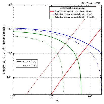
Figure 1: Average kinetic energy gain induced by a single encounter with the Galactic disk as a function of $r/r_{s}$, for two NFW subhalos ($10^{-6}$ and $10^{6}M_{\odot}$) located at $R_{\odot}$ – see the definition in Eq. (48) (here, we use the M11 mass model parameters). Also shown are their gravitational potentials. We plot the results in units of $G_{N}\,\rho_{s}\,r_{s}^{2}$, which comes out as a natural scaling, to make the comparison more striking.

The calculations presented above are at the basis of the methods we propose to follow to account for disk shocking, and thereby to further prune or destroy subhalos. Below, we discuss two different strategies, which we will call differential and integrated disk shocking to make the distinction clear. Common to both methods is the number of disk crossings, $N_{\rm cross}$, which is computed from the circular velocity of a subhalo in the Galactic frame (we implicitly assume circular orbits) and the age of the Galaxy $T_{\rm MW}$:

$$N_{\rm cross}(R)=\sqrt{\frac{G_{N}\,M(R)}{R}}\,\frac{T_{\rm MW}}{\pi\,R}\,.$$ (49)

Throughout this paper, we will set $T_{\rm MW}=10$ Gyr. Assuming the M11 Milky Way mass model described in Sect. III.2, the number of disk crossings is $\sim(670,92,37)$ for Galactocentric radii $R\in(1\,{\rm kpc},R_{\odot},20\,{\rm kpc})$, respectively. This already tells us that disk shocking will lead to more efficient tidal stripping for subhalos which venture toward the central parts of the Galaxy.

Besides the disk-shocking methods presented below, which are aimed to determine subhalo tidal radii in Galactic regions encompassing the baryonic disk, our tidal disruption criteria will be discussed in Sect. III.4.4 where the disk-shocking methods will be further compared.

Tidal radius from differential disk shocking.

The so-called differential disk-shocking method will be our primary method, and relies on a comparison between the kick in velocity induced by disk shocking, as effectively described in Eq. (48), and the escape velocity

$$v_{\rm esc}(r)=\sqrt{-2\,\tilde{\phi}(r)}\,.$$ (50)

If the kick induced by disk shocking is such that the particle reaches the escape velocity, then it gets unbound to the system. Therefore, for each disk crossing, we will accordingly define the tidal radius as the radius at which the kick in velocity equals the escape velocity. In terms of energies, this reads

$$r_{t}\;\text{such that}\;\langle\epsilon_{k}\rangle(r_{t})=-\tilde{\phi}(r_{t})\,.$$ (51)

This procedure must be applied at each crossing, such that it may somehow capture the dynamics of disk shocking. Indeed, hidden in $\tilde{\phi}$ [see Eq. (28)] is the radial boundary of the subhalo, which means that the above equation must be applied iteratively up to the number $N_{\rm cross}$ of disk crossings given in Eq. (49). More explicitly, we have for the $i^{\rm th}$ crossing

$$r_{t,i}\;\text{such that}\;\langle\epsilon_{k}\rangle(r_{t,i})=-\tilde{\phi}(r_{t,i},r_{t,i-1})\,.$$ (52)

In practice, we start with the tidal radius inferred from the global tidal effects induced by the host halo and discussed in Sect. III.4.1. This method can easily be applied to any subhalo model, irrespective of the inner density profile. It also provides a dynamical description of disk shocking, while only approximately. Indeed, this iterative procedure assumes that the internal structure of the shocked subhalo is not altered between two crossings, while part of the energy could actually be redistributed. Anyway, this picture is still consistent with adiabatic invariance, which partly protects the inner parts of subhalos against tidal pruning.

An illustration of this differential disk-shocking method is shown in Fig. 1, where we have plotted the disk-shocking energy $\langle\epsilon_{k}\rangle(r)$ (red curves) and the gravitational potential modulus $|\tilde{\phi}(r)|$ as a function of the scaling variable $r/r_{s}$ (where $r_{s}$ is the subhalo scale radius). We have considered two different NFW subhalos, $10^{-6}$ (solid curves) and $10^{6}M_{\odot}$ (dashed curves), both located at $R_{\odot}$. The corresponding gravitational potential moduli are evaluated using two different radial boundaries for subhalos, one set to $r_{200}$ (blue curves), and the other set to $r_{200}/10$ (green curves), above which they are exponentially suppressed — the $1/r$ scaling expected beyond $r_{s}$ is poorly seen as the potential goes from $\propto{\rm cst}$ to $\propto(1/r-1/r_{t})\approx e^{-r/r_{t}}/r$ very fast. These radial boundaries can be thought of as initial tidal radii before disk crossing such that the blue curves illustrate the potential energies before the first crossing, while the green curves show how they have evolved after one or several crossings. By virtue of Eq. (51), the tidal radius after one disk crossing will be set to the radius at which the kinetic energy and the potential curves intersect. Therefore, Fig. 1 nicely illustrates why the tidal stripping efficiency is much larger (i) in the outer regions of the system (compare where the red curves intersect the blue curves – first crossing), and (ii) for more massive subhalos (compare the relative level at which the red curves intercept the green curves – subsequent crossings). The former effect is a consequence of the the regular increase of the differential disk-shocking energy as $\propto r^{2}$ which will at some point encounter the decreasing potential, stripping off the right-hand part of the DM content (the shift between the $10^{-6}/10^{6}\,M_{\odot}$ red solid/dashed curves is merely due to the difference in $r_{s}$); instead, the latter effect is due to the fact that lighter subhalos are either much less extended and more concentrated, such that after the first crossings, the further reduced disk shocking energy (because of the smaller internal radius $r$, as it scales $\propto r^{2}$) makes only a tiny fraction of the residual potential and only prunes the very external parts of small subhalos.

All this shows, in particular, that the impact of the number of crossings is important, though quite not linear in this differential approach. The implementation of this method will represent our primary tool to account for disk-shocking effects.

Tidal radius from integrated disk shocking.

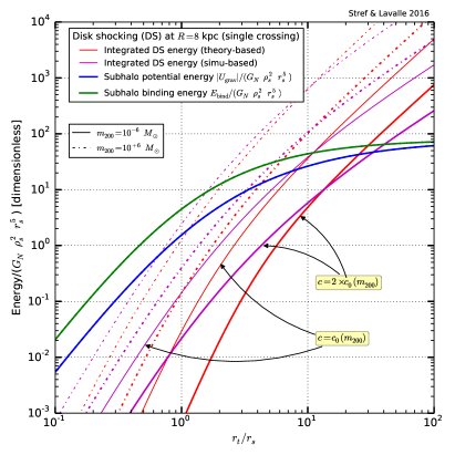
Figure 2: Integrated kinetic energy gain induced by the Galactic disk as a function of $r_{t}/r_{s}$, for two NFW subhalos ($10^{-6}$ and $10^{6}M_{\odot}$) located at 8 kpc, assuming two different concentration values (the median one, and twice the median) — see the definitions in Eq. (53) for the theory-based calculation, and see Eq. (55) for the simulation-based estimate. Also shown are the binding and potential energies. We plot the results in units of $G_{N}\,\rho_{s}^{2}\,r_{s}^{5}$, which leads to the same binding and potential energies for both subhalo masses.

In contrast to what was presented above as a differential disk-shocking method, we can now try to integrate the kinetic energy gain over the whole subhalo – hence the term integrated disk shocking method. Such a method was partly followed in Ref. Berezinsky et al. (2008), where the authors used the Eddington equation in the isothermal limit to convert the energy gain in phase space into a mass loss. Here, instead, we will use spherical symmetry, and simply assume that WIMPs take only circular orbits, such that the integrated kinetic energy gain can be expressed as

$$E_{k}(r_{t},R)=2\,\pi\int_{0}^{r_{t}}dr\,r^{2}\int_{-1}^{1}d\cos(\theta)\,\epsilon_{k}(z,R)\,\frac{\rho(r)}{m_{\chi}}\,,$$

(53)

where $\epsilon_{k}(z,R)$ is given by Eq. (47), and $\rho$ is the inner subhalo mass density profile. Spherical symmetry merely implies that $z^{2}=r^{2}\cos^{2}(\theta)$, which makes the computation easy. This integrated energy gain can then be compared to the binding energy or to the potential energy, for each subhalo. For an NFW profile, the scaling goes from roughly $\propto\rho_{s}\,r_{s}^{5}\,(r_{t}/r_{s})^{4}$ for $r_{t}\ll r_{s}$, to $\propto\rho_{s}\,r_{s}^{5}\,(r_{t}/r_{s})^{2}$ for $r_{t}\gg r_{s}$.

This is illustrated for a single disk crossing in Fig. 2, for two subhalos of $10^{-6}$ (solid curves) and $10^{6}M_{\odot}$ (dash-dotted curves) located about the solar position – for completeness, we use two different concentration values for each subhalo: the median value (thin curves), and twice the median (thick curves). The red curves show the integrated disk-shocking energy given in Eq. (53), as compared to the binding (green curve) and potential (blue curve) energies [see Eqs. (26) and (27), and the associated comments about the radial scaling]. Using units of $G_{N}\,\rho_{s}^{2}\,r_{s}^{5}$ allows us to get a single curve for each of the latter energies, for both subhalo masses. Again, the increase in the disk-shocking energy is such that it will encounter the binding energy, which flattens beyond $r_{s}$, thereby setting a tidal radius. As well depicted from Fig. 2, smaller as well as more concentrated objects will be less prone to tidal stripping, which can be understood from working out the scaling $E_{b}(r_{t})/E_{k}(r_{t})\propto\rho_{s}\,(r_{t}/r_{s})^{-a}\propto c^{3}\,(r_{t}/r_{s})^{-a}$, where $a\approx 3$ [see discussion just below Eq. (53)]. This explains why, like it was already the case for differential disk shocking, more massive subhalos will be more efficiently affected by tidal stripping.

Since we are dealing with integrated energies, we define the subhalo tidal radius after $N_{\rm cross}$ disk crossings as

$$r_{t}\;\text{such that}\;N_{\rm cross}\,E_{k}(r_{t},R)=E_{b}(r_{t})\,,$$ (54)

where we use the binding energy $E_{b}$ defined in Eq. (26) as a reference.

Tidal radius from integrated disk shocking (fits on cosmological simulations).

For the sake of comparison, we now introduce a result fitted on dark-matter-only zoomed-in cosmological simulations, given in Ref. D’Onghia et al. (2010), wherein a baryonic disk potential was grown adiabatically to study the induced tidal disruption of subhalos. The qualitative features of this result were recently recovered in cosmological simulations including baryons, and discussed in Ref. Zhu et al. (2016). The authors of Ref. D’Onghia et al. (2010) have tried to capture disk-shocking effects by a simple and physically motivated ansatz, which, as they found, matches rather well with their simulation results (see e.g. Ref. Binney and Tremaine (2008) for the dynamical grounds). They introduced an integrated-like disk-shocking energy $\tilde{E}_{k}(r_{t},R)$ given by

$$\frac{\tilde{E}_{k}(r_{t},R)}{E_{b}(r_{t})}=\frac{(1.84\,r_{1/2})^{2}\,g_{z,{\rm disk}}^{2}}{3\,\tilde{\sigma}_{v}^{2}\,V_{z}^{2}}\,,$$ (55)

where $r_{1/2}$ is the radius containing half the subhalo mass, $g_{z,{\rm disk}}$ is the disk gravitational force field given in Eq. (39), $\tilde{\sigma}$ is an estimate of the internal dispersion velocity given by $\tilde{\sigma}^{2}=0.4\,G_{N}\,m_{t}/r_{1/2}$, and $V_{z}$ is the velocity component perpendicular to the disk, which will be inferred from the approximation given in Eq. (44). This disk-shocking energy is shown as the purple curves in Fig. 2, for the two subhalo prototypes introduced above. It still scales more sharply with $r_{t}$ (readily inferred as $\propto r_{t}^{3}$ from the equation just above) than the potential or binding energy, though less sharply than the integrated disk-shocking energy discussed in the previous paragraph, while still with a similar amplitude around $r_{t}/r_{s}\simeq 10$. This means that this way to implement disk shocking will likely disrupt subhalos more efficiently, as gravitational stripping toward the central regions becomes more efficient. Still, we note that Eq. (55) relies on fits on simulation results, and could therefore be more specific to the subhalo mass range probed by cosmological simulations, which is still strongly limited by resolution issues. Anyway, the resulting subhalo tidal radius after $N_{\rm cross}$ disk crossings can then be calculated by means of Eq. (54), by simply replacing $E_{k}(r_{t},R)$ with $\tilde{E}_{k}(r_{t},R)$.

Disk-shocking summary.

We have introduced the so-called differential and integrated disk-shocking energies. For the latter, we have derived two expressions, one consistent with the differential one, and another inspired by cosmological simulation and fully independent. These physical quantities allow us to derive the subhalo tidal radius $r_{t}$ after $N_{\rm cross}$ disk crossings for any method. These calculations lead to different results, but common to all is the fact that $r_{t}$ does depend simultaneously on the subhalo mass $m$, its concentration $c$, its position in the Galaxy $R$, and its internal density profile. Our primary method will be the one based on the differential disk-shocking energy, as it relies on fewer assumptions. We will compare all these results in Sect. III.4.4.

III.4.3 Subhalo mass independence of $x_{t}=r_{t}/r_{s}$

A striking property of all the tidal radius calculation methods discussed above, both those involving global tides and those involving disk shocking, is that the ratio $x_{t}=r_{t}/r_{s}$ turns out to be independent of the subhalo mass. Actually, $x_{t}$ depends only on the subhalo concentration $c$ and on its radial position $R$ in the Galaxy. If the latter dependence is rather easy to understand (tidal stripping depends on the position), the former is much less trivial.

For the global tides discussed in Sect. III.4.1, it is easy to show that the methods based on the Jacobi limit can be formulated along

$$x_{t} = \left[\frac{\Delta_{200}\,f(x_{t})}{\Delta_{t}(R)\,f(c)}\right]^{1/3}\,\kappa\,c$$

$$\Leftrightarrow x_{t}\,\left[f(x_{t})\right]^{-1/3} = \left[\frac{\Delta_{200}}{\Delta_{t}(R)\,f(c)}\right]^{1/3}\,\kappa\,c\,,$$

which makes it clear that $x_{t}$ is only a function of $R$ and $c$. Here, $\kappa=r_{-2}/rs$ is set by the choice of the inner profile, and the function $f$ can be defined on general grounds by means of the subhalo mass, $m(x)=4\,\pi\,\rho_{s}\,r_{s}^{3}\,f(x)$, where $x=r/r_{s}$ – for an NFW profile, it is simply $f(x)=\ln(1+x)-x/(1+x)$. We have also defined $\Delta_{x}=\langle\rho\rangle_{r_{x}}/\rho_{c}$, i.e. the ratio of the average subhalo density within a radius $r_{x}$ to the critical density ($\Delta_{200}=200$). In the case of the pointlike Jacobi approximation corresponding to the tidal definition of Eq. (35), for instance, we have

$$\Delta_{t}(R)=9\,M/(4\,\pi\,R^{3}\,\rho_{c})\,,$$

where $M$ is the whole host galaxy mass.

The demonstration for the method of setting the tidal radius by equating the inner density to the outer density, given in Eq. (37), is trivial, and relies on the fact that the subhalo scale density $\rho_{s}$, regardless of its profile and its mass, is only set by the concentration parameter — for an NFW profile, it reads

$$\rho_{s}=\frac{\Delta_{200}\,\rho_{c}}{3}\,\frac{c^{3}}{f(c)}\,.$$

If we write the density profile as $\rho(r)=\rho(x=r/r_{s})=\rho_{s}\,u(x)$, then Eq. (37) translates into $u(x)=\rho_{\rm tot}(R)/\rho_{s}$, which makes it clear again that $x_{t}$ depends only on $c$ and $R$.

Finally, the cases of disk-shocking tidal effects are more subtle. In the differential method, $x_{t}$ can readily be shown to be a function of $c$ and $R$ only from Eq. (51). This is simply because the potential $\tilde{\phi}(r_{t})\propto r_{s}^{2}g(x_{t},c)$, where it is not necessary to specify function $g$, while the kinetic energy $\langle\epsilon_{k}\rangle(r_{t})\propto r_{t}^{2}\,\bar{g}(x_{t},c,R)$, with the function $\bar{g}$ being unspecified too, such that equating them leads to an equation that involves only the variables $x_{t}$, $c$ and $R$. This proves that $x_{t}$ only depends only on $c$ and $R$. The reasoning is similar for the so-called integrated disk-shocking methods, and also leads to the dependence only on $R$ and $c$ of the associated $x_{t}$. Note that the independence of $x_{t}$ on the subhalo mass cannot be read off Fig. 1 nor off Fig. 2 because subhalos with different masses in these plots have also different concentrations.

III.4.4 Tidal disruption criterion and minimal concentration

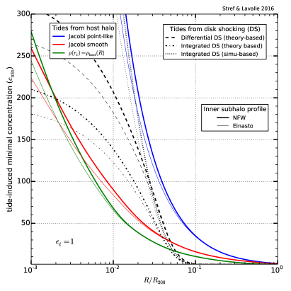
Figure 3: Minimal concentration as a function of the dimensionless galactocentric radius $R/R_{200}$, induced by different tidal effects. The solid curves show the global tides effects discussed in Sect. III.4.1, and the non-solid curves show the disk-shocking effects discussed in Sect. III.4.2. See more comments in Sect. III.4.4.

Equipped with several tidal radius definitions, we can now define a tidal disruption criterion by specifying the function $\zeta(r_{t})$ introduced in Eq. (24), where $r_{t}$ is the subhalo tidal radius. We remind the reader that the latter depends on all the specific subhalo properties, and on its position in the host halo. In light of results obtained in Ref. Hayashi et al. (2003), we may define the following very simple disruption function:

$$\zeta\left(x_{t}\equiv\frac{r_{t}}{r_{s}}\right)\equiv\theta\left(x_{t}-\varepsilon_{t}\right)\,,$$ (56)

where $\theta$ is the usual dimensionless step function, $r_{s}=r_{s}(m,c)$ is the subhalo scale radius, and the parameter $\varepsilon_{t}$ sets the minimal value allowed for $x_{t}$. This parameter very likely depends on the inner subhalo density profile, and could also depend on the specific process responsible for tidal stripping. Typical values found using dark-matter-only simulations are $\varepsilon_{t}\approx 2$ (see Ref. Hayashi et al. (2003)), but we may wonder whether simulations can efficiently capture the continuous limit due to their limited spatial/mass resolution. For definiteness, we will set $\varepsilon_{t}=1$ in the following, unless specified otherwise.

This translates into a minimal bound on the subhalo concentration, $c_{\rm min}(R)$, as the surviving subhalos are only those with scale radii such that $r_{t}/r_{s}\geq\varepsilon_{t}$. This concentration cutoff reads

$$c_{\rm min}(R)=\frac{\varepsilon_{t}}{\kappa}\,\frac{r_{200}(m)}{r_{t}\left(c_{\rm min}(R),m,R\right)}\,,$$ (57)

a transcendental equation that can be solved iteratively. Here, $\kappa=r_{-2}/r_{s}$ is fixed by the choice of density profile ($\kappa=1$ for an NFW or an Einasto profile). In practice, we will further impose that

$$c_{\rm min}(R)={\rm Max}\left\{c_{\rm min}(R);1\right\}\,.$$ (58)

We emphasize that $c_{\rm min}$ does not actually depend on the subhalo mass, but only on its location $R$ in the Galaxy. This is because $x_{t}$ is only a function of the concentration $c$ and $R$, as explained in Sect. III.4.3.

This concentration lower bound, $c_{\rm min}(R)$, is the very variable that differentiates the tidal stripping methods discussed in Sect. III.4.1 and in Sect. III.4.2. We report our calculations of $c_{\rm min}$ in Fig. 3, as a function of the dimensionless Galactic radius $R/R_{200}$ ($R_{200}=237$ kpc in the M11 model). The curves related to the global tides are shown as solid colored lines, while those associated with disk shocking are the nonsolid ones. Note that we have also included the baryons in the calculation of the global tide effects (see Sect. III.4.1). We also stress that we preformed the calculation assuming two different inner subhalo profiles: an NFW profile (thick curves), and an Einasto profile (thin curves) — we took an index of $\alpha_{e}=0.17$ for the latter. From the plot, there is no significant qualitative difference between these profiles, except that Einasto subhalos are very slightly more resistant to gravitational tides.

We note that the most approximate method for the global tides, the pointlike Jacobi limit given in Eq. (35), is also the one that destroys subhalos most efficiently, even more efficiently than disk shocking in the central parts of the Galaxy. It can therefore be used for fast and conservative calculations, although it is highly sensitive to the estimate of the total mass of the Galaxy, which is often ambiguous as it depends on the choice for the virial radius. To make the discussion more quantitative, we recall that a $10^{-6}M_{\odot}$ subhalo has a peak concentration of $\sim 60$, which will serve as a reference value here. We see from the plot that the pointlike tide method affects such tiny objects already from $20$ kpc and selects in only exponentially high concentration, while disrupting less concentrated objects. This means that at the solar position all subhalos have already been almost fully disrupted. The two other global tides methods [given in Eqs. (III.4.1) and (37)], which are much more realistic, give similar results and lead to much less tidal stripping than the pointlike approximation. Subhalos of $10^{-6}M_{\odot}$ start to be strongly affected around 2-4 kpc from the MW center in these scenarios.

Disk-shocking effects start to play a role only from $20$ kpc inward, as expected from the typical gravitational size of the Galactic disk. All disk-shocking methods lead to more stripping than global tidal effects, except for the pointlike approximation discussed above. Here again, we see that the most approximate method, the integrated disk-shocking method fitted on cosmological simulations and given in Eq. (55), is the most efficient for destroying or pruning subhalos. Besides being based on very crude approximations, we stress that it is also likely biased by the resolution limit inherent to cosmological simulations, where only subhalos with masses $\gtrsim 10^{4-7}$ can be tracked. These massive objects are much less concentrated than their lighter brothers and sisters, and more prone to stripping and disruption. In contrast, the less efficient method is the one based on integrated disk shocking and given in Eq. (54). Intermediate is the method most motivated on theoretical grounds. Interestingly, the latter starts to deplete subhalos of $10^{-6}M_{\odot}$ around the position of the Sun.

In summary, global tides tend to dominate the stripping beyond the disk, while disk shocking dominates inward. This was obviously expected, but we quantified and illustrated these effects rather exhaustively. Moreover, we showed that the pointlike Jacobi approximation makes it irrelevant to include disk shocking, as it supersedes all other effects over the whole Galactic range. Nevertheless, as we discussed above, this pointlike approximation is by far the worst to make, while being conservative. Obviously, in a consistent and complete model, one has to include all tides, those coming from global gravitational effects, and those coming from disk shocking. This is what we will do when discussing our final results in Sect. IV.

III.4.5 Tidal selection of the most concentrated objects: Shift of the average concentration

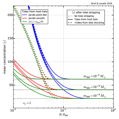
Figure 4: Mean concentration as a function of the dimensionless Galactocentric radius $R/R_{200}$, induced by different tidal effects. The solid curves show the global-tides effects discussed in Sect. III.4.1, and the non-solid curves show the disk-shocking effects discussed in Sect. III.4.2. See more comments in Sect. III.4.4.

By depleting the lower tail of the concentration distribution, tidal effects modify the average concentration of subhalos as a function of their mass. This can be explicitly calculated by means of the first moment of the concentration function, given in Eq. (III.3.1). The increase in the average concentration merely comes from the fact that tidal effects reduce the concentration range from below by $c_{\rm in}(R)\geq 1$. In reality, the concentration function should not be truncated that sharply, but this truncation still captures the main physical effects at play.

We illustrate this in Fig. 4, where we report our calculations of $\langle c(m)\rangle$ as a function of the dimensionless Galactic radius $X_{200}=R/R_{200}$ for three different subhalo masses, $10^{-6}$, $1$, and $10^{6}M_{\odot}$, and for all the tidal-stripping methods introduced above. The asymptotic values of $\langle c(m)\rangle$ at $X_{200}\to 1$ correspond to the average concentration computed in the range $c_{\rm min}=1$, $c_{\rm max}=\infty$. As we go inward, tidal effects come into play and $c_{\rm min}$ increases, leading to the increase in $\langle c(m)\rangle$. Recalling that the concentration function is Gaussianly suppressed beyond the median value $c_{0}(m)\approx$10-100, in the considered subhalo mass range, we can therefore read off from the plot that most of subhalos with masses larger than that of a given curve are tidally depleted as the curve exceeds $\sim 100$. This trend is consistent with previous studies performed from dark-matter-only cosmological simulation results (see e.g. Refs. Hayashi et al. (2003); van den Bosch et al. (2005); Diemand et al. (2007a); Kamionkowski et al. (2010); Moliné et al. (2016); Jiang and van den Bosch (2016)), or from simple analytic approximations (see e.g. Ref. Bartels and Ando (2015)), but these works did not include baryonic effects. Here we provide quantitative estimates for both baryonic and dark matter tidal effects, and comparisons between different approaches.

III.4.6 Impact of tidal effects on the calibration and normalization procedure

It may prove useful to summarize the way tidal effects are integrated in the full procedure in practice. As discussed in Sect. III.2.3, we calibrate the subhalo population by considering only the so-called global tidal effects presented in Sect. III.4.1. These global tidal effects translate into a function $c_{\rm min}^{0}(R)$ that cuts the concentration PDF from below and allows us to determine both $N_{\rm sub}^{0}$ and the associated normalization of the whole subhalo phase space $K_{0}$. This must be done without baryons at all, consistently with the fact that the calibration is based upon dark-matter-only simulation results. Then, we compute the final phase-space normalization $K$ that accounts for the baryonic tides (both the global tide and the disk-shocking calculations), which are characterized by a new cutoff function $c_{\rm min}(R)$. We obtain the final number $N_{\rm sub}$ of subhalos by demanding that the overall subhalo mass density be unaffected at very large radii, far from the disk, where baryonic effects can be neglected. This can be rephrased as setting $N_{\rm sub}=(K/K_{0})\,N_{\rm sub}^{0}$.

III.5 Reference Galactic halo model (including a subhalo population)

Before discussing in detail the observables relevant to DM searches in the next section, we define here our reference Galactic model:

• Our reference Galactic mass model, which fixes both the global dark halo (including subhalos) and the Galactic baryonic content is the M11 model (see Sect. III.2).

• Global tides induced by the global mass distribution are by default calculated in the smooth Jacobi limit [see Sect. III.4.1 and Eq. (III.4.1)].

• Tides induced by disk shocking will be calculated by default with the differential disk-shocking method [see Sect. III.4.2 and Eq. (52)].

• The default tidal disruption efficiency will be set to $\varepsilon_{t}=1$ [see Sect. III.4.4 and Eq. (56)].

Any result in the following will derive from this default configuration unless specified otherwise. We will also consider two benchmark cases for the initial mass index, $\alpha_{M}=1.9$ and $\alpha_{M}=2$. Similarly, we will consider two benchmark cutoff subhalo masses, $m_{\rm min}=10^{-6}\,M_{\odot}$ and $m_{\rm min}=10^{-10}\,M_{\odot}$.

IV Concrete results: Mass profiles, number density profiles, luminosity profiles, and boost factors

In the previous section, we introduced the whole scheme to derive a Galactic subhalo population consistently with current dynamical constraints, assuming only a smooth-halo component and spherical symmetry. This scheme was integrated in a C++ numerical code, and in this section, we will present our main results. In Sect. IV.1, we will first inspect the overall subhalo mass profile that comes out as a result of our tidal-stripping procedure. Then, in Sect. IV.2, we will present the corresponding subhalo number density profile. Finally, in Sect. IV.3, we will show how the obtained subhalo distribution translates into an annihilation profile, and subsequently quantify the associated annihilation boost factor. Throughout this section, we will also comment on the specific impacts of the initial subhalo mass distribution index $\alpha_{M}$ and the minimal subhalo mass (see Sect. III.3.2).

IV.1 Mass profiles

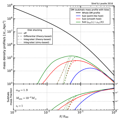
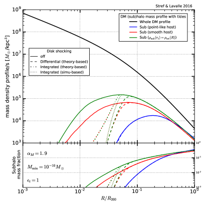
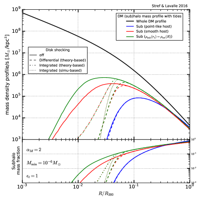
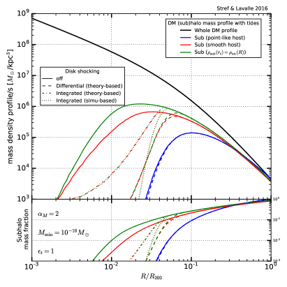
Figure 5: Mass profiles obtained for different subhalo configurations as embedded in the M11 Galactic mass model. Top (bottom) panels illustrate our results for a mass index of $\alpha_{M}=1.9$ (2, respectively). Left (right) panels adopt a minimal subhalo mass of $m_{\rm min}=10^{-6}\,M_{\odot}$ ($10^{-10}\,M_{\odot}$, respectively). All panels: the black solid curve shows the constrained overall dark halo mass density profile, and the other curves feature the global contribution of subhalos for different tidal effect calculations. Blue, red, and green curves illustrate the global tides induced by the dark halo itself calculated respectively in the pointlike Jacobi limit, the smooth Jacobi limit, and the density equality limit discussed in the text (see Sect. III.4.1). Dashed, dashed-dotted and dotted curves show additional impact of the gravitational stripping induced by disk shocking respectively based on the differential method, the integrated method, and the empirical fit done on simulation results; these methods are discussed in Sect. III.4.2.

Mass function index	Total number	Phase-space normalization	Fraction in	Total mass fraction
$\alpha_{M}$	of surviving subhalos	$K_{w}$	local density (average)	within $R_{200}$
$\alpha_{M}=1.9$	$5.19\times 10^{18}$	0.9638	0.04%	14.69%
$\alpha_{M}=2$	$2.84\times 10^{20}$	0.9639	0.84%	47.88%

Table 3: Results for our subhalo model as embedded in the M11 Galactic configuration, when all tidal effects are included (see reference model configuration in Sect. III.5). Here, we take a cutoff subhalo mass of $10^{-10}M_{\odot}$, and a tidal disruption efficiency of $\varepsilon_{t}=1$.

In Sect. III.1, we have introduced the smooth and subhalo dark matter components from the overall density profile $\rho_{\rm tot}$ in Eq. (2), which we rewrite with an explicit spherical symmetry to make the present discussion clear:

$$\rho_{\rm tot}(R)=\rho_{\rm sm}(R)+\rho_{\rm sub}(R)\,.$$ (59)

We remind the reader that $\rho_{\rm tot}$ is subject to dynamical constraints, and we have adopted the M11 model as a template Galactic mass model (see Sect. III.2). The smooth dark matter component $\rho_{\rm sm}$ featured above can only be derived a posteriori, after having determined the subhalo component $\rho_{\rm sub}$ given in Eq. (12). Making the tidal cutoff $c_{\rm min}(R)$ explicit, the latter reads

$$\rho_{\rm sub}(R) = \frac{N_{\rm sub}}{K_{w}}\,\frac{d{\cal P}_{V}(R)}{dV}\,\int_{m_{\rm min}}^{m_{\rm max}}dm\int_{c_{\rm min}(R)}^{c_{\rm max}}dc\,m_{t}(r_{t}(c,m,R),m,c)\,\frac{d{\cal P}_{m}}{dm}\,\frac{d{\cal P}_{c}}{dc}$$

$$\text{with}\;K_{w} = 4\,\pi\int_{0}^{R_{200}}dR\,R^{2}\,\frac{d{\cal P}_{V}(R)}{dV}\int_{m_{\rm min}}^{m_{\rm max}}dm\int_{c_{\rm min}(R)}^{c_{\rm max}}dc\,\frac{d{\cal P}_{m}}{dm}\,\frac{d{\cal P}_{c}}{dc}\,,$$ (60)

where $N_{\rm sub}$ is the total number of subhalos, $m_{t}$ is the subhalo mass contained in the tidal radius $r_{t}$, and the ${\cal P}$’s define the global subhalo phase space, normalized to unity thanks to $K_{w}$, introduced in Sect. III.2.2. Taking the M11 Galactic mass model as a reference, the associated prediction of the overall subhalo mass density profile is shown in Fig. 5, where we also represent the impact of the mass index ($\alpha_{M}=1.9/2$ in the top/bottom row’s panels) and that of the minimal subhalo mass ($10^{-6}/10^{-10}M_{\odot}$ in the left/right column’s panels). In each panel, we give predictions for all the methods introduced in Sect. III.4 to compute the tidal stripping and associated subhalo disruption – the upper part of each plot shows the mass density profile, and the lower part shows the subhalo mass fraction, as functions of the dimensionless Galactic radius $R/R_{200}$. Subhalo mass profiles relying only on global tides are reported as solid colored curves – see Sect. III.4.1 – while those incorporating disk-shocking effects as well are shown as dashed (differential), dash-dotted (integrated), and dotted (simulation-fit inspired method) – see Sect. III.4.2. We recall that our reference model is based on the global tides evaluated in the smooth Jacobi limit (dubbed smooth host in the plots), given in Eq. (III.4.1), and on the differential disk-shocking method given in Eq. (52). It is represented as dashed red curves in each panel. Some illustrative numbers can also be found in Tab. 3.

Overall, these results show that tidal effects strongly deplete the subhalo population in the central parts of the Galaxy, and underline the impact of disk shocking, which plays an important role. This gives rise to a cored-like spatial distribution inward, before the full disruption of subhalos in the very center ($\lesssim 4$ kpc). These are generic features observed in cosmological simulations, but our analytic procedure allows us to make predictions down to much lower spatial and mass scales, in a dynamically constrained and consistent frame. Going to more specific global tidal stripping configurations, we see that the global pointlike Jacobi method, which is clearly too approximate as it does not account for the host halo and subhalo profiles’ details, disrupts almost all subhalos within $R/R_{200}\lesssim 0.1\Leftrightarrow R\lesssim 20$ kpc, making disk-shocking effects even irrelevant. This strongly suppresses the local ($R/R_{200}\sim 0.3$-0.4) subhalo mass fraction, typically to $\ll 1\%$. The two other more physically motivated global methods provide slightly more optimistic predictions, with a local subhalo mass fraction $\sim 10\%$. When disk-shocking effects are further included, however, it decreases down to $\lesssim 1\%$. Still, we will see in Sect. IV.3 that this low fraction is somewhat compensated for, in terms of annihilation rate, by a tidal selection of more concentrated objects. The impact of the minimal subhalo mass is only noticeable for a mass index of 2, as most of the mass fraction is then carried by the smallest objects, which are much more resilient to tidal effects. Since the minimal subhalo mass can in principle be determined by the interaction properties of WIMPs (more or less straightforwardly related to its mass), most of the theoretical uncertainties are then featured by $\alpha_{M}$. For our reference model, we see that while the mass fraction can vary by a factor of $\sim 2$ between $\alpha_{M}=1.9$ and $\alpha_{M}=2$ in the outskirts of the Galaxy, its differential value is much more sensitive because of more efficient tidal selection of lighter subhalos. In the latter case, the variation can reach an order of magnitude. This should have an impact on predictions for direct subhalo searches (see e.g. Refs. Feldmann and Spolyar (2015); Clark et al. (2016b)).

Finally, we note that the amount of subhalo mass lost during disk crossings could in principle be quantified from our method, which may be used to size the impact of the smallest pruned subhalos on the high tail of the WIMP velocity distribution (see e.g. Refs. Zemp et al. (2009); Kuhlen et al. (2010)). Indeed, disk shocking induces a net kinetic energy gain for the pruned WIMPs. This, however, goes beyond the scope of this work.

IV.2 Number density profiles

Another interesting observable complementary to the mass profile discussed above is the number density profile, which will provide another angle to understand the role of tides and their immediate consequences. In Eq. (11), we provided the differential subhalo number density as a function of the cosmological mass $m=m_{200}$, which is not the actual tidal subhalo mass $m_{t}$. It is easy to show that $m$ and $m_{t}$ are related by

$$m_{t}=m\,\Delta(\vec{x},c)\,,$$ (61)

where function $\Delta(\vec{x},c)\leq 1$ encodes the dependence of $m_{t}$ (or $r_{t}$) on position and concentration. Since this dependence factorizes, one can merely trade the phase-space volume $dV\,dm\,dc$ for $dV\,dm_{t}\,dc$ by means of the classical Jacobian. This is equivalent to the projection of $dn_{\rm sub}/dm$ on $dn_{\rm sub}/dm_{t}$ directly by means of the delta function $\delta(m_{t}-m_{200}\,\Delta(\vec{x},c))$. Note that physically, different masses $m$ and different concentrations $c$ will lead to to the same tidal mass $m_{t}$, which means that the cosmological nature of the initial mass spectrum is somewhat erased by tidal stripping.

We get

$$\frac{dn_{\rm sub}(\vec{x},m_{t})}{dm_{t}}=\frac{N_{\rm sub}}{K_{w}}\,\frac{d{\cal P}_{V}(\vec{x})}{dV}\,\int_{m_{\rm min}}^{m_{\rm max}}dm\,\int_{c_{\rm min}(\vec{x})}^{c_{\rm max}}dc\,\frac{d{\cal P}_{c}}{dc}\,\big{|}{\cal J}_{m_{t}/m}\big{|}\,\frac{d{\cal P}_{m}(m)}{dm}\,\delta(m-m_{t}/\Delta(\vec{x},c))\,,$$ (62)

where the Jacobian $\big{|}{\cal J}_{m_{t}/m}\big{|}=\Delta(\vec{x},c)$, and where the dependence on position $\vec{x}$ amounts in our study to a dependence in radial position $R$.

It is straightforward to verify that

$$n_{\rm sub}(\vec{x})=\int_{m_{\rm min}}^{m_{\rm max}}dm\frac{dn_{\rm sub}(\vec{x},m)}{dm}=\int_{m_{t,{\rm min}}}^{m_{t,{\rm max}}}dm_{t}\frac{dn_{\rm sub}(\vec{x},m_{t})}{dm_{t}}\,,$$ (63)

which shows the consistency of Eq. (62) with Eq. (11). In the equation above, the maximal tidal mass $m_{t,{\rm max}}$ can be set to $m_{\rm max}$ while the minimal tidal mass $m_{t,{\rm min}}$ can readily be obtained from $m_{\rm min}$:

$$m_{t,{\rm min}}(\vec{x})=m_{\rm min}\,\Delta(\vec{x},c_{\rm min}(\vec{x}))\leq m_{\rm min}\,.$$ (64)

The differential number density profile $dn_{\rm sub}/dm_{t}$ is actually proportional to a local mass distribution that we can defined as a locally normalized function

$$\frac{d\widetilde{\cal P}_{m}(m,\vec{x})}{dm} = \frac{d{\cal P}_{m}(m)}{dm}\frac{\int_{c_{\rm min}(\vec{x})}^{c_{\rm max}}dc\,\frac{d{\cal P}_{c}}{dc}}{\int_{m_{\rm min}}^{m_{\rm max}}dm\,\frac{d{\cal P}_{m}(m)}{dm}\,\int_{c_{\rm min}(\vec{x})}^{c_{\rm max}}dc\,\frac{d{\cal P}_{c}}{dc}}$$

$$\frac{d\widetilde{\cal P}_{m_{t}}(m_{t},\vec{x})}{dm_{t}} = \frac{\int_{c_{\rm min}(\vec{x})}^{c_{\rm max}}dc\,\frac{d{\cal P}_{c}}{dc}\,\big{|}{\cal J}_{m_{t}/m}\big{|}\,\frac{d{\cal P}_{m}(m)}{dm}\,\delta(m-m_{t}/\Delta(\vec{x},c))}{\int_{m_{\rm min}}^{m_{\rm max}}dm\,\int_{c_{\rm min}(\vec{x})}^{c_{\rm max}}dc\,\frac{d{\cal P}_{c}}{dc}\,\big{|}{\cal J}_{m_{t}/m}\big{|}\,\frac{d{\cal P}_{m}(m)}{dm}\,\delta(m-m_{t}/\Delta(\vec{x},c))}\,,$$ (65)

where we have given both the virial $d\widetilde{\cal P}_{m}/dm$ and tidal $d\widetilde{\cal P}_{m_{t}}/dm_{t}$ functions, and where the numerators ensure the local normalization to unity. We see from the above equation that the spatial-dependence of the range in concentration induced by $c_{\rm min}(\vec{x})$ will modify the mass index $\alpha_{M}$ which characterizes the initial mass function $d{\cal P}_{m}/dm$ given in Eq. (32), leading to an effective mass index $\widetilde{\alpha}_{M}(\vec{x})\geq\alpha_{M}$, because the more massive subhalos will be more efficiently disrupted toward the central parts of the Galaxy. This is illustrated in Fig. 6, where we report $m^{2}dn_{\rm sub}/dm$ (in terms of both the cosmological and tidal masses) at different positions: inside the disk ($R=8$ kpc), at the very end of the disk ($R=20$ kpc), and far from the disk ($R=100$ kpc). The initial mass index has been fixed to $\alpha_{M}=2$, but the qualitative behavior would be the same with 1.9. The initial mass distribution is explicitly reflected in the dotted curves, which show the differential number density before tidal stripping is applied, and which are flat in the graph because of the $m^{2}$ rescaling (here, we took the same total number of subhalos as for the global tides-only case). There is a sharp cutoff corresponding to the minimal subhalo mass ($10^{-10}/10^{-6}\,M_{\odot}$ in the left/right panel). The difference in amplitude between these dotted curves only comes from the difference in the spatial distribution value, which initially scales like $\rho_{\rm tot}$ (the amplitude increases as the radius $R$ decreases). As tidal effects are plugged in, the dotted curves are converted to the dashed curves, still in terms of the cosmological mass $m=m_{200}$. While these curves are close to each other at $R=100$ kpc (black curves), we see a departure of the tidal curve below intermediate masses at $R=20$ kpc (red curves), and finally a very strong departure over the whole mass range at $R=8$ kpc (blue curves). The latter exhibits a local effective mass index $\widetilde{\alpha}_{M}\sim 3\gg\alpha_{M}$, and a strongly depleted amplitude, such that despite the initially much larger number density at $R=8$ kpc, the hierarchy is now reverted. This reflects the impact of tidal disruption whose efficiency is strongly enhanced in the disk because of disk shocking. We stress that this only illustrates the behavior of the local effective mass index. When integrated over the whole halo, the effect would still be visible but much less pronounced because of the significant weight carried by subhalos located far from the disk, leading to a global effective mass index $\gtrsim\alpha_{M}$, as obtained in other studies (see e.g. Jiang and van den Bosch (2016); van den Bosch and Jiang (2016)). Still, it is striking to see how tidal effects deeply affect the phase space locally.

So far, we discussed Fig. 6 in terms of cosmological mass. If we now concentrate on the differential subhalo number density in terms of real (tidal) mass $m_{t}$ (solid curves), the picture gets modified. The most noticeable difference comes from the fact that the boundary is less sharp at low masses, and that this boundary does not coincide with $m_{\rm min}$ anymore, but can be much lower (depending on the tidal disruption parameter $\varepsilon_{t}$ – see Sect. III.4.4). If fact, only subhalos with very large concentrations will have $m_{t}\sim m$, so subhalos located at a given position on the cosmological-mass curve will migrate toward the left part of the tidal-mass curve as their concentration decreases. Therefore, $m_{t}$ no longer carries cosmological information by itself, only the internal structure of subhalos does. Moreover we emphasize that only $dn_{\rm sub}/dm_{t}$ is a directly observable quantity, not $dn_{\rm sub}/dm$. Though not obvious from the graphs, the differential number density curves reported in Fig. 6 do obey the consistency relation given in Eq. (63).

Finally, if we perform the mass integral of $dn_{\rm sub}/dm$, we can get the subhalo number density profile $n_{\rm sub}(r)$ in the Milky Way [see Eq. (63)]. We illustrate this in Fig. 7, where we report results for different configurations, all assuming the M11 Galactic mass model: without tidal effects (dotted curves), with global tides only (dashed curves), with global tides and disk shocking (solid curves); for two different values of the mass index $\alpha_{M}$ (1.9/2 for the green/blue curves), and two values for the minimal cutoff mass ($m_{\rm min}=10^{-6}\,M_{\odot}/10^{-10}\,M_{\odot}$ for the left/right panel). For tidal effects, we used the reference modeling summarized in Sect. III.5. The cases with tidal effects do not strictly converge toward the case without tides because the latter comes with a slightly smaller total number of subhalos as a normalization bias (it is calculated by requiring the same mass fraction in a reference range as in the global tides-only case, though without stripping or disruption allowed, hence more subhalos – see Sect. III.2.3). The difference induced by $m_{\rm min}$ is simply in the relative amplitude of the number density, as explained in more detail in Sect. IV.5.

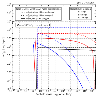
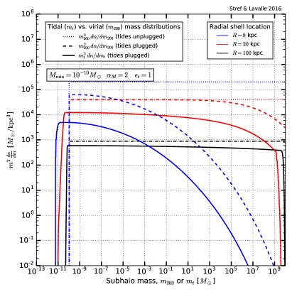
Figure 6: Left panel: mass-differential number density in terms of both the cosmological mass $dn_{\rm sub}/dm$ (dotted/dashed curves for tidal effects unplugged/plugged) and the real tidal mass $dn_{\rm sub}/dm$ (solid curves), assuming a cutoff mass $m_{\rm min}=10^{-6}\,M_{\odot}$, and calculated at 3 positions ($R=8/20/100$ kpc in blue/red/black), as a function of the relevant mass (a scaling of $m^{2}$ is applied as $\alpha_{M}=2$ is chosen here). Right panel: same as in the left panel but with $m_{\rm min}=10^{-10}\,M_{\odot}$.

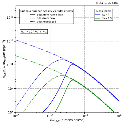
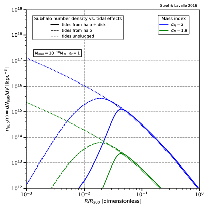
Figure 7: Left panel: Subhalo number density profile assuming the M11 Galactic mass model (dotted/dashed/solid curves for tidal effects unplugged/halo/halo+disk from the reference model – see Sect. III.5), two different cases for the mass index $\alpha_{M}$ (1.9/2 for the green/blue curves), and assuming a cutoff mass $m_{\rm min}=10^{-6}\,M_{\odot}$. Right panel: same as in the left panel but with $m_{\rm min}=10^{-10}\,M_{\odot}$.

IV.3 Annihilation rate profiles and boost factors

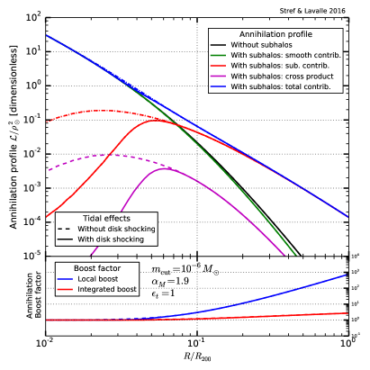
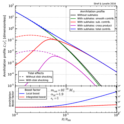
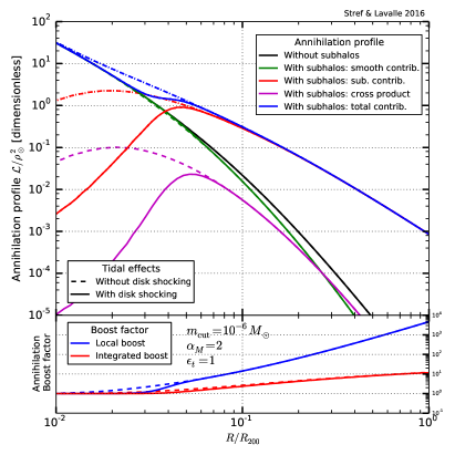
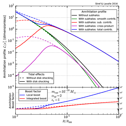
Figure 8: Annihilation/luminosity profiles for different assumptions. Upper part of each panel: Black curves show the profile when neglecting subhalos, blue curves show the overall profile when subhalos are included and all tidal effects are considered, green curves show the separate contribution of the smooth halo, red curves show the contribution of subhalos, and magenta curves the contribution of the subhalo-smooth halo cross product. Dashed lines show the impact of neglecting disk-shocking effects. Lower part of each panel: Differential (blue curves) and integrated (red curves) boost factors. Upper/lower row: $\alpha_{M}=1.9/2$. Left/right panels: Minimal subhalo mass of $10^{-6}/10^{-10}M_{\odot}$.

In this section, we discuss the potential enhancement the presence of dark matter subhalos may induce in the WIMP annihilation rate in the Galaxy, usually dubbed the boost factor. Here, we will only determine the differential and integrated boost factors on the annihilation rate, not on the observable cosmic-ray or gamma-ray fluxes. We remind the reader that in terms of these fluxes, the annihilation boost factor is angular dependent for gamma rays Bergström et al. (1999), while it is energy dependent for antimatter cosmic rays Lavalle et al. (2007, 2008).

In this work, we will assume that subhalos do not superimpose, such that we will not account for the potential existence of sub-subhalos, which might be relevant in the most massive subhalos, as they have formed at later epochs than the lightest ones. We still stress that any inclusion of sub-subhalos should be consistent with the normalization and calibration procedures one subscribes to (in particular, the overall mass function should be recovered after all layers of subhalos have been accounted for). With this assumption, the total annihilation rate can be derived starting from a discrete distribution of $N_{\rm sub}$ subhalos, where the total dark matter density would be given by

$$\rho_{{\rm tot},N_{\rm sub}}(\vec{x})=\rho_{\rm sm}(\vec{x})+\sum_{i}^{N_{\rm sub}}M_{t,i}\delta(\vec{x}-\vec{x}_{i})\,,$$ (66)

where each subhalo $i$ is pointlike and allocated a tidal mass $M_{t,i}$, and $\rho_{\rm sm}$ is the smooth dark matter density. Squaring this equation, we get

$$\rho_{{\rm tot},N_{\rm sub}}^{2}(\vec{x})=\rho_{\rm sm}^{2}(\vec{x})+\sum_{i\geq j}^{N_{\rm sub}}M_{t,i}\delta(\vec{x}-\vec{x}_{i})\,M_{t,j}\delta(\vec{x}-\vec{x}_{j})+2\,\rho_{\rm sm}(\vec{x})\sum_{i}^{N_{\rm sub}}M_{t,i}\delta(\vec{x}-\vec{x}_{i})\,.$$ (67)

Neglecting sub-subhalos formally implies that $\vec{x}_{i}\neq\vec{x}_{j}\,\forall\,i\neq j$. If we now take the continuous limit and make spherical symmetry explicit, we obtain

$$\rho_{\rm tot}^{2}(R) = \rho_{\rm sm}^{2}(R)$$ (68)

$$+\frac{N_{\rm sub}}{K_{w}}\,\frac{d{\cal P}_{V}(R)}{dV}\,\int_{m_{\rm min}}^{m_{\rm max}}dm\,\frac{d{\cal P}_{m}(m)}{dm}\int_{c_{\rm min}(R)}^{\infty}dc\,\frac{d{\cal P}_{c}(c,m)}{dc}\,\int_{0}^{r_{t}(R,c,m)}dr\,4\,\pi\,r^{2}\,\left\{\rho^{2}(r)+2\,\rho(r)\,\rho_{\rm sm}(R)\right\}$$

$$= \rho_{\rm sm}^{2}(R)+N_{\rm sub}\,\frac{d{\cal P}_{V}(R)}{dV}\,\left\{\rho^{2}_{\odot}\widetilde{\langle\xi_{t}\rangle}(R)+2\,\rho_{\rm sm}(R)\,\widetilde{\langle m_{t}\rangle}(R)\right\}$$

where $m_{t}$ and $\xi_{t}$ are the subhalo tidal mass and annihilation volume, defined in Eqs. (24) and (25) respectively. The symbol $\widetilde{\langle\rangle}$ denotes the averaging over the concentration and mass parts of the subhalo phase space, made explicit in Eq. (12), which is position dependent. Notice the crossing term above induced by the interaction between subhalos and the host halo. Usually assumed to be subleading and thereby neglected, it may actually dominate over the smooth contribution at large Galactic radii, as will be shown below. We now define the dimensionless WIMP luminosity ${\cal L}$, which measures the spatial dependence of the annihilation rate, as

$${\cal L}(R)\equiv\frac{\rho_{\rm tot}^{2}(R)}{\rho^{2}_{\odot}}\,,$$ (69)

where the normalization $\rho_{\odot}$ is made at the solar position. We further introduce the differential annihilation boost factor ${\cal B}(R)$, and the integrated annihilation boost factor $B(R)$, as

$${\cal B}(R) \equiv \frac{{\cal L}(R)}{{\cal L}_{\text{no sub.}}(R)}\,,$$ (70)

$$B(R) = \frac{\int_{0}^{R}dr\,r^{2}\,{\cal L}(r)}{\int_{0}^{R}dr\,r^{2}\,{\cal L}_{\text{no sub.}}(r)}\,.$$

Defined so, these boost factors are merely the multiplicative corrections to apply to the differential or integrated annihilation rate as computed by neglecting the subhalo component. Note that in principle, any WIMP signal prediction involving subhalos should be affected by a statistical variance, reflecting the possible fluctuations of the number of contributing objects Lavalle et al. (2007, 2008). We keep this aspect for further dedicated studies.

We report our calculation results for the annihilation profiles in Fig. 8, where we again adopt M11 as the reference Galactic mass model — this is the translation of Fig. 5 in terms of annihilation profiles. Global tides are calculated from the smooth Jacobi method [see Eq. (III.4.1)], while disk-shocking effects are described from the differential method [see Eq. (52)]. The top (bottom) row’s panels correspond to a subhalo mass index of 1.9 (2). The left (right) column’s panels correspond to a minimal subhalo mass of $10^{-6}M_{\odot}$ ($10^{-10}M_{\odot}$). In each panel, the upper part shows the different components of the annihilation profile, and the lower part shows the differential and integrated boost factors as defined above. We display the impact of neglecting disk shocking as dashed curves, which demonstrates the importance of this effect in the central parts of the Galaxy.

A generic result is that the subhalo contribution dominates at large radii, typically from the edge of the Galactic disk for a subhalo mass index of $\alpha_{M}=1.9$, and even from much more inner regions in the case of $\alpha_{M}=2$. For an overall NFW profile, this leads to a characteristic scaling of $1/r^{2}$ toward the Galactic center, where the smooth halo dominates, progressively changing to $1/r^{3}$ outward, when the luminosity profile tracks the subhalo spatial distribution. Interestingly, in the case of $\alpha_{M}=2$, where the global subhalo luminosity is enhanced, a plateau arises in the overall luminosity profile at the transition between smooth-halo domination and subhalo domination. This is actually an imprint of disk-shocking effects, which delay the rising of the subhalo contribution. We will see later that this plateau does not depend on the tidal disruption efficiency, and is also preserved in the case of an overall Einasto profile. This striking feature might be used in gamma-ray searches.

Finally, we comment on our results for the differential and integrated boost factors. The so-called differential boost factor (reported as “local” in the plots) is mostly relevant to indirect dark matter searches with antimatter cosmic rays because of the limited horizon of the latter induced by propagation effects. It also represents the correction to apply to the integrand of the line-of-sight integral used in gamma-ray searches. On the other hand, the integrated boost is related to the absolute Galactic luminosity, and thereby also to extragalactic gamma-ray searches — then the Galaxy appears as a template case characterizing other galaxies close in mass. We see that at the solar position ($R/R_{200}\sim 0.03$-0.04), the boost is locally $<2$ for $\alpha_{M}=1.9$, while it reaches $\sim 5$ for $\alpha_{M}=2$. Though moderate, these values may have some impact on the existing limits on WIMPs as the precision in the cosmic-ray data has strongly increased in recent years. We also remark that the differential boost increases up to $10^{3}$-$10^{4}$ toward the edge of the Galaxy, which strongly affects, for instance, the diffuse gamma-ray signal at high Galactic latitudes, as known from long ago (see e.g. Refs. Bergström et al. (1999); Pieri et al. (2011)). Regarding the integrated boost, the values obtained at the edge of the dark halo can represent useful calibration values for calculations of the dark matter contribution to the extragalactic diffuse gamma-ray flux. These go from $\sim 3$ for $\alpha_{M}=1.9$, to $\sim 20$ for $\alpha_{M}=2$. This is fully consistent with the recent study in Ref. Moliné et al. (2016) (see Fig. 6 in this article), which is based on fits of cosmological simulations, and does not include baryonic effects – while global tides are merely the outcomes of the simulations themselves. That baryons play no role in the integrated boost at the whole Galactic scale should not come as a surprise, as they only affect the dynamics in the very central parts of the halo.

At this stage, we have illustrated our results assuming a tidal efficiency of $\varepsilon_{t}=1$ [see Eq. (56)]. It is important to check their stability against changes in this parameter. In Fig. 9, we investigate the impact of $\varepsilon_{t}$ by computing the annihilation profiles for $\varepsilon_{t}=0.5$ (subhalos can be pruned down to $r_{s}/2$ before getting disrupted), and for $\varepsilon_{t}=2$ (subhalos can be pruned only down to $2\times r_{s}$ before getting disrupted). We adopt the configuration for which the plateau discussed above is visible, namely $\alpha_{M}=2$. We see that the plateau is slightly smeared when $\varepsilon_{t}=0.5$, as disk-shocking effects are then less disruptive and smear the previously abrupt rising of the subhalo contribution. On the contrary, the plateau is much more salient when $\varepsilon_{t}=2$, as expected. Values of 0.5 are rather small compared to what is found in cosmological simulations (see e.g. Ref. Hayashi et al. (2003)), but they could be relevant, for instance, to the very concentrated cores of ultracompact minihalos, close to the minimal cutoff mass (see e.g. Ref. Berezinsky et al. (2014) for further discussion). Nevertheless, we see that except close to the smooth-halo/subhalo luminosity domination transition, changes in $\varepsilon_{t}$ have no significant impact on our predictions. In particular, the plateau feature does not seem to be spoiled.

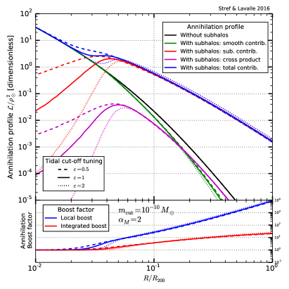
Figure 9: Impact of the tidal disruption efficiency on the annihilation profile [see Eq. (56)]. Decreasing values of $\varepsilon$ imply a less efficient disruption (tidal pruning allowed down to smaller radii).

IV.4 Comparison between different Galactic mass models

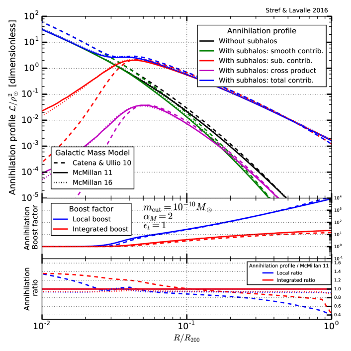
Figure 10: Comparison of the annihilation profiles for different Galactic mass models (M11, CU10, and M16 – see text for details). Annihilation profiles are normalized to the $\rho_{\odot}^{2}$ of each model. The lower panel shows the real relative difference of each configuration with the M11 setup.

Throughout this study, we have adopted the M11 Galactic mass model as a reference. It is interesting to check how our predictions are affected by changes in the Galactic model itself, while still trying to use dynamically constrained scenarios. To this aim, we will use two other Galactic models: (i) that of Ref. Catena and Ullio (2010) (CU10 hereafter), which is particularly interesting as it relies on an Einasto dark halo instead of an NFW one, and (ii) the upgraded and updated version of M11, recently released in Ref. McMillan (2016) by the same author (M16 henceforth), still based on an NFW profile for the dark halo, but with additional constraints from novel kinematic data. Besides the details of the dark matter halo profile and the data sets used as dynamical constraints, changes with respect to M11 also come from the additional inclusion of a two-component gaseous disk (HI and HII) in both models. Including gas actually has no significant impact on the dark matter profile on large scales, as this mostly tunes the distribution of the inner overall gravitational potential among all, baryonic and dark, components. Rather, this mostly influences the understanding of very local stellar dynamics. Note that since the gas components of CU10 are directly inferred from data points, we will instead, for convenience, use those of M16 in both M16 and CU10, which may be described from Eq. (6). (We further trade the original vertical sech² of M16 for an exponential function, which has no impact on the final result). The sets of parameters of these models are given in Tab. 1 and Tab. 2.

Concrete comparisons are displayed in Fig. 10 in terms of annihilation and boost-factor profiles, where solid (dashed and dotted) curves correspond to M11 (CU10 and M16, respectively) predictions. We adopt the “best-case” configuration, where $\alpha_{M}=2$ and the cutoff subhalo mass is $10^{-10}M_{\odot}$. The color code is the same as in Fig. 8. Luminosity profiles are measured in units of the squared dark matter density $\rho_{\odot}^{2}$ at the solar position $R_{\odot}$, which (barely) change from one model to another. The upper horizontal axes feature the Galactic radius in units of $R_{200}$, which also varies between configurations – see Tab. 1. We add another lower panel that provides the real annihilation profile ratio with respect to M11, where the luminosity is then evaluated at the corresponding M11 radius for each model – consequently, the lower horizontal axis features $R/R_{200}$ as inferred from M11 only.

We first notice that the difference between M11 and M16 is hardly visible, and amounts to $\lesssim 10\%$ over the full Galaxy, M16 being slightly less luminous in terms of dark matter annihilation. This is not surprising as the only changes between M11 and M16 are the addition of a gaseous disk and a new set of constraining data. On the other hand, differences are more pronounced between CU10 and M11-M16: CU10 is brighter than M11-M16 in the central parts of the Galaxy, typically for $R/R_{200}<0.1$. This is obviously a consequence of the different halo shape, as Einasto profiles are known to be more luminous than NFW profiles within the scale radius (except for the divergence of NFW profiles at the very centers – see e.g. Ref. Pieri et al. (2011)), while having a faster luminosity decrease outward because of the exponential cutoff in the halo shape. This amounts to an increase of $\sim 20\%$ in integrated luminosity at the Solar position, and a decrease of the same order at the edge of the Galaxy. In terms of boost factors, which measure the impact of subhalos relative to the host halo and therefore can be directly compared between different mass models, we see that the difference is very moderate for the differential boost, leading to an integrated difference $<2$ at the edge of the dark halo (CU10 leads to a slightly smaller integrated boost factor).

Finally, we remark that the plateau feature emphasized in Sect. IV.3 as a signature of a sharp subhalo mass function also shows up in CU10, despite the different overall halo shape. This prediction is therefore robust against systematic uncertainties in the overall dark halo modeling, provided the smooth halo density continues increasing inward, where the subhalo population has been fully depleted — this plateau could convert into a bump for a cored smooth halo profile.

IV.5 Impact of the minimal cutoff mass

As mentioned in Sect. III.3.2, the minimal cutoff mass $m_{\rm min}$ of subhalos should be related to the very properties of the DM particle (production mechanism, interaction properties). In principle, one can calculate this cutoff mass for each candidate Chen et al. (2001); Hofmann et al. (2001); Berezinsky et al. (2003); Green et al. (2004); Loeb and Zaldarriaga (2005); Boehm and Schaeffer (2005); Profumo et al. (2006); Bertschinger (2006); Bringmann and Hofmann (2007); Bringmann (2009); Berezinsky et al. (2014); Visinelli and Gondolo (2015), so it is not, strictly speaking, a free parameter once the underlying theory is fixed, even though equal-mass particles would come with minimal mass scale varying by orders of magnitude Bringmann (2009). Nevertheless, it is still interesting to summarize the impact of $m_{\rm min}$ on our results. The following discussion assumes that the initial spectral mass index is fixed to a single value $\alpha_{M}>1$, so that the structure mass spectrum is regular – note that some inflation or phase transition scenarios may predict more complex patterns for the primordial perturbation spectrum on small scales which should imprint the mass spectrum, strongly affecting the way we described the initial mass function (see e.g. Ricotti and Gould (2009) and further exploration of this framework in Aslanyan et al. (2016)); we will not discuss these cases here.

Since we have calibrated the subhalo population by fixing a mass fraction in a reference mass range (see Sect. III.2.3), and since the maximal subhalo mass is $m_{\rm max}\gg m_{\rm min}$ it is easy to show that the total number of subhalos scales like $N_{\rm sub}\overset{\sim}{\propto}m_{\rm min}^{1-\alpha_{M}}$, and hence the number density profiles $n_{\rm sub}(r)$ shown in Fig. 7. Tidal effects will simply affect the relative fraction of the less massive objects with respect to the more massive ones toward the central regions of the Galaxy, as shown in Fig. 6. This is reflected by the local modification of the initial mass index, as discussed below Eq. (65).

For the mass profiles shown in Fig. 5, the impact of $m_{\rm min}$ can be inferred from the relation $\rho_{\rm sub}\overset{\sim}{\propto}N_{\rm sub}\,\langle m\rangle\approx{\rm cst}$, with $\langle m\rangle\overset{\sim}{\propto}m_{\rm min}^{\alpha_{M}-1}\,\ln(m_{\rm max}/m_{\rm min})$ (we have assumed $\alpha_{M}\sim 2$ to get the log). Given the scaling of $N_{\rm sub}$ discussed just above, this helps understand that despite the striking difference in terms on number density, the mass profile is instead rather similar for $m_{\rm min}=10^{-6}\,M_{\odot}$ and $m_{\rm min}=10^{-10}\,M_{\odot}$. Indeed, the small difference induced by $m_{\rm min}$ on $\rho_{\rm sub}$ comes from the logarithmic correction (a factor of 4/5) and also from tidal stripping which is more efficient for more massive subhalos, of which the relative population is further reduced in the latter case, hence a slightly larger amplitude for the corresponding mass profiles. This difference is a bit more pronounced for $\alpha_{M}=2$ because of the logarithmic term discussed above, which is replaced by $\sim m_{\rm max}^{2-\alpha_{M}}$ for $\alpha_{M}=1.9$, further reducing the impact of $m_{\rm min}$.

Finally, the dependence of the annihilation profiles depicted in Fig. 8 in $m_{\rm min}$ can be understood from the subhalo mass dependence of its annihilation luminosity, which for an NFW profile is ${\cal L}_{i}\overset{\sim}{\propto}m_{i}^{0.9}$ Lavalle et al. (2008). Since the total luminosity ${\cal L}\overset{\sim}{\propto}N_{\rm sub}\,\langle{\cal L}_{i}\rangle$, then we get ${\cal L}\overset{\sim}{\propto}m_{\rm min}^{1.9-\alpha_{M}}$, which explains why the annihilation profiles do not exhibit significant dependence on $m_{\rm min}$ when $\alpha_{M}=1.9$, while it is more noticeable for $\alpha_{M}=2$.

V Conclusions

We have proposed a method to model a galactic dark matter subhalo population consistently with dynamical constraints, focusing on the Milky Way – subhalos are unavoidable galactic components if dark matter is made of WIMPs or any other dark matter candidates with suppressed self-interactions and devoid of additional pressure. Dynamical consistency is important to make sense of constraints or discovery potentials of both direct and indirect dark matter searches (see e.g. Ref. Lavalle and Magni (2015) for an illustration in direct searches). We have assumed that subhalos initially track the host halo profile when the galaxy forms and then we have explicitly calculated the effects of tidal stripping and subsequent potential disruption induced not only by the overall gravitational potential but also by baryonic disk crossing. We have developed and compared different theoretical approaches to deal with the latter, and retained the so-called differential disk-shocking method as our reference case, since it is built upon more accurate physical grounds. This method was inspired by previous works dedicated to the understanding of stellar clusters, in particular by Refs. Ostriker et al. (1972); Weinberg (1994a); Gnedin and Ostriker (1999); Gnedin et al. (1999b, a). These references were already used in other analytic studies (see e.g. Ref. Berezinsky et al. (2008)), but were dealt with in a significantly different way, leading to a different formulation of tidal mass losses without explicit links to the definition of a tidal radius. Nevertheless, even if it is difficult to make quantitative comparisons between the mentioned study and ours, it seems that both approaches are in agreement at least at the qualitative level. Our study was more aimed at quantifying the impact of a subhalo population on the dark matter annihilation rate and sizing the related theoretical uncertainties in a realistic Galactic mass configuration, while Ref. Berezinsky et al. (2008) was more concerned with the survival probability of subhalos against different types of tidal effects. On the whole, our method to include disk-shocking effects is likely simpler to implement in numerical calculations. A summary of the method is given in Sect. II.

The main inputs of our model are (i) the Galactic mass model, (ii) the subhalo mass function, and (iii) the subhalo concentration function, for which we adopted consensual prescriptions. Further assumptions regard the choice of the inner subhalo profile. We considered a spherically symmetric host halo, hence a spherically symmetric subhalo distribution. Our model can in principle easily be extended to axisymmetric host halos, while its numerical implementation will then likely become much trickier. We stress that we calibrated the subhalo mass fraction using constraints from cosmological simulations without baryons. It is important to use dark-matter-only simulations because baryonic components in hydrodynamic simulation are likely to differ significantly from those of the real Milky Way, while strongly affecting the dynamics of subhalos: it would then become impossible to disentangle the global from other tidal effects, and it would make it spurious to calibrate a subhalo population model a posteriori. This underlines the need to continue running dark-matter-only simulations with increased resolution and up-to-date cosmological parameters, even in a context where issues related to the impact of baryons on cold dark matter halos are certainly the most pressing ones.

Using the recent and constrained Galactic mass models from Refs. McMillan (2011); Catena and Ullio (2010); McMillan (2016) (dubbed M11, CU10, and M16 – M11 being used as the template case), characterized by different assumptions on the dark halo profile while providing results consistent with each other, we computed the overall subhalo mass profiles and further made predictions for the induced annihilation profiles. We stress that these results incorporate a self-consistent calculation of the tidal radius for each subhalo, depending on its mass, concentration, and position in the Galaxy; individual mass and luminosity are calculated up to the tidal radius for each subhalo. We used different assumptions for the mass index $\alpha_{M}$ and the cutoff subhalo mass. Since the latter could in principle be determined from WIMP interaction properties in specific scenarios, the main theoretical uncertainty is actually carried by $\alpha_{M}$. Based on our reference model summarized in Sect. III.5, we showed that the global or integrated boost factor could vary between $\sim 2$ (for $\alpha_{M}=1.9$) and $\sim 20$ (for $\alpha_{M}=2$, respectively) for all choices of Galactic mass models. This may provide interesting and complementary calibration points for estimates of the dark matter contribution to the extragalactic diffuse gamma-ray background (see e.g. Ref. Ajello et al. (2015)). We also derived differential boost factors (i.e. the boost factor profile) that could be used to revisit estimates of the dark matter contribution to the Galactic diffuse gamma-ray emission (e.g. Refs. Charbonnier et al. (2012); Ackermann et al. (2012, 2015); Fornasa et al. (2016); Cirelli et al. (2015)), or to the local antimatter cosmic-ray flux (e.g. Refs. Boudaud et al. (2015b); Giesen et al. (2015); Kappl et al. (2015); Evoli et al. (2015)). Interestingly, our model predicts a plateau in the overall annihilation rate in the case of a sharp mass function ($\alpha_{M}=2$) that could lead to specific observable effects. This feature seems to persist within the considered theoretical and systematic uncertainties of the model.

The local subhalo population and induced boost factor, relevant to direct searches and antimatter searches, respectively, are very sensitive to $\alpha_{M}$. For antimatter searches, though, the precision achieved in the most recent measurements is such that even a moderate effect could have a significant impact on the existing limits or discovery prospects. In the most optimistic case, when $\alpha_{M}=2$, the enhancement can reach a factor of 10 (the impact of the cutoff subhalo mass $m_{\rm min}$ is discussed in Sect. IV.5).

It would be interesting to test this model against cosmological simulations with baryons in the relevant subhalo mass range in the near future, but this is clearly beyond the scope of the present study. In any case, the model is easily tuneable in terms of initial distribution functions, provided internal consistency with the dynamical constraints, which was the main purpose of this work. Finally, self-made predictions for direct and indirect dark matter searches are left to further studies.