Behaviour of hot electrons under the dc field in chiral carbon nanotubes

Abstract

Behaviour of hot electrons under the influence of dc field in carbon nanotubes is theoretically considered. The study was done semi-classically by solving Boltzmann transport equation with the presence of the hot electrons source to derive the current densities. Plots of the normalized axial current density versus electric field strength of the chiral CNTs reveal a negative differential conductivity (NDC). Unlike achiral CNTs, the NDC occurs at a low field about $\mathrm{6\ kV/cm}$ for chiral CNT. We further observed that the switch from NDC to PDC occurs at lower dc field in chiral CNTs than achiral counterparts. Hence the suppression of the unwanted domain instability usually associated with NDC and a potential generation of terahertz radiations occurs at low electric field for chiral CNTs.
Keywords: Hot electrons, Nanotubes, Negative Differential Conductivity

Introduction

Carbon nanotubes (CNTs) which are unique tubular structures of nanometric diameter with an extremely high length-to-diameter aspect ratio [1] have a wide variety of possible applications [2, 3, 4]. The primary symmetry classification of carbon nanotubes is as either being achiral (symmorphic) or chiral (non-symmorphic) [5]. Each type of CNT can be either metallic or semiconducting depending on their diameter and rolling helicity  [6]. Much progress has been made recently showing that carbon nanotubes (CNTs) are advanced quasi-$1$D materials for future high performance electronics [4, 7, 13]. The behaviour of hot electrons in electronic devices has been observed since the arrival of the transistor in $1947$ [14]. A number of devices have been proposed whose very principle is based on effects of hot electrons [15]. In this paper, we present theoretical framework investigations of behaviour of hot electrons under the influence of dc field in chiral carbon nanotubes using the semiclassical Boltzmann transport equation. We probe the behaviour of the electric current density mainly due to the presence of hot electrons in chiral CNTs as a function of the applied dc field along the axis of the tube.

1 Theory

Suppose hot electrons is injected axially in a chiral carbon nanotube which is considered as an infinitely long chains of carbon atoms wrapped along a base helix under the influence of dc field $E$ . The current densities in axial and circumferential directions are calculated by adopting semiclassical approximation approach. In the presence of hot electrons source, the motion of quasiparticles in dc field is described by Boltzmann transport equation in the form [16, 17]:

$$\frac{\partial f(p)}{\partial t}+v_{p}\frac{\partial f(p)}{\partial r}eE(t)\frac{\partial f(p)}{\partial p}=-v[f(p)-f_{0}(p)]+S(p)$$ (1)

where $v=1/\tau,v$ is the scattering frequency of the electrons, $\tau$ is relaxation time of electrons, $S(p)$ is the hot electrons source function, $f(p)$ is distribution function, $f_{0}(p)$ is equilibrium distribution function, $\nu_{p}$ is the electron velocity, $r$ is the electron position, $p$ is the electron dynamical momentum, $e$ is the electronic charge and t is time elapsed. The energy $\varepsilon(p)$ of the electrons, calculated using the tight binding approximation is given as expressed in [18] for a chiral carbon nanotubes:

$$\varepsilon(p)=\varepsilon_{0}-\triangle_{s}\cos(\frac{p_{s}d_{s}}{\hbar})-\triangle_{z}\cos(\frac{p_{z}d_{z}}{\hbar})$$ (2)

where $\varepsilon_{0}$ is the energy of an outer-shell electron in an isolated carbon atom, $\triangle_{z}$ and $\triangle_{s}$ are the real overlapping integrals for jumps along the tubular axis and the base helix respectively, $p_{s}$ and $p_{z}$ are the components of carrier momentum tangential to the base helix and along the tubular axis respectively. $\hbar=h/2\pi$ and $h$ is Planck’s constant. $d_{s}$ and $d_{z}$ are the distances between the atomic sites $n1$ and $n1+1$, $n_{s}$ and $n_{s}+N_{0}$ respectively along the base helix and the tubular axis where, $(N_{0}>1)$. The components $v_{s}$ and $v_{z}$ of the electron velocity $v_{p}$ in equation ($1$) are respectively calculated from the energy dispersion relation equation ($2$) as

$$v_{s}(p_{s})={\partial\varepsilon(p)\over\partial p_{s}}={\triangle_{s}d_{s}\over\hbar}\sin({p_{s}d_{s}\over\hbar})$$ (3)

$$v_{z}(p_{z})={\partial\varepsilon(p)\over\partial p_{s}}={\triangle_{z}d_{z}\over\hbar}\sin({p_{z}d_{z}\over\hbar})$$ (4)

In accordance with [18, 19, 20, 21], we find that the distribution function is periodic in the quasi-momentum and can be written in Fourier series as:

$$f_{0}(p_{s},p_{z})={n_{0}d_{s}d_{z}\over 2I_{0}({\triangle_{s}\over k_{B}T})I_{0}({\triangle_{z}\over k_{B}T})}\sum^{\infty}_{\alpha=-\infty}I_{\alpha}({\triangle_{s}\over k_{B}T})\sum^{\infty}_{\beta=-\infty}I_{\beta}({\triangle_{z}\over k_{B}T})\times$$

$$\exp\{i\alpha p_{s}d_{s}/\hbar+\beta p_{zd_{z}}/\hbar\}$$ (5)

$$f_{0}(p_{s},p_{z},t)={n_{0}d_{s}d_{z}\over 2I_{0}({\triangle_{s}\over k_{B}T})I_{0}({\triangle_{z}\over k_{B}T})}\sum^{\infty}_{\alpha=-\infty}I_{\alpha}({\triangle_{s}\over k_{B}T})\sum^{\infty}_{\beta=-\infty}I_{\beta}({\triangle_{z}\over k_{B}T})\times$$

$$\exp\{i\alpha p_{s}d_{s}/\hbar+\beta p_{zd_{z}}/\hbar\}\emptyset_{\alpha}(t)$$ (6)

where $f(p_{s},p_{z},t)$ is the distribution function, and $f_{0}(p_{s},p_{z})$ is the equilibrium distribution function, $\emptyset_{\alpha}(t)$ is the factor by which the Fourier transform of the non-equilibrium distribution function differs from its equilibrium distribution counterpart, $I_{\alpha,\beta}$ is the modified Bessel function of order the ${\alpha,\beta}$, where $\alpha,\beta=0,1,...$, $n_{0}$ is equilibrium particle density and $k_{B}$ is Boltzmann constant. We consider a hot electron source $S(p)$ of the simplest form given by the expression [17]

$$S(p)=Q\delta(p-p\prime)-{Q\over n_{0}}f_{s}(p)$$ (7)

where $f_{s}(p)$ is the stationary solution of Eqn.($1$), $Q$ is the injection rate of hot electrons and $p\prime$ and $p$ are their momentum. In the case of constant electric field, the solution to Eqn. ($1$) becomes

$$\emptyset_{\alpha}(p_{s},p_{z})={n_{0}d_{s}d_{z}\over 2I_{0}({\triangle_{s}\over k_{B}T})I_{0}({\triangle_{z}\over k_{B}T})}\sum^{\infty}_{\alpha=-\infty}I_{\alpha}({\triangle_{s}\over k_{B}T})\sum^{\infty}_{\beta=-\infty}I_{\beta}({\triangle_{z}\over k_{B}T})\times$$

$${v\over(v+ie\alpha dE)}\exp\{i\alpha p_{s}d_{s}/\hbar+\beta p_{zd_{z}}/\hbar\}$$ (8)

Therefore Eqn.($6$) becomes

$$f_{E}(p_{s},p_{z})={n_{0}d_{s}d_{z}\over 2I_{0}({\triangle_{s}\over k_{B}T})I_{0}({\triangle_{z}\over k_{B}T})}\sum^{\infty}_{\alpha=-\infty}I_{\alpha}({\triangle_{s}\over k_{B}T})\sum^{\infty}_{\beta=-\infty}I_{\beta}({\triangle_{z}\over k_{B}T}){v\over(v+ie\alpha dE)}$$

$$\times\exp\{i\alpha p_{sd_{s}}/\hbar+\beta p_{zd_{z}}/\hbar\}$$ (9)

The stationary homogeneous distribution function $f_{s}(p)$ in the presence of hot electron source Eqn.($7$) is given by

$$f_{s}(p)=f_{E}(p)+f^{\prime}(p)$$ (10)

Substituting Eqn.($10$) into Eqn.($1$) we get

$${\partial f^{\prime}(\varphi)\over\partial\varphi}+({v\over\Omega}+{Q\over n_{0}\Omega})f^{\prime}(\varphi)={d_{s}Q\over\Omega}\delta(\varphi-\varphi^{\prime})-{Q\over\Omega n_{0}}f(\varphi)$$ (11)

$\Omega=\Omega_{s,z}={ed_{s,z}E\over\hbar}$ and $d_{s,z}$ is bandwidth, $\varphi$ and $\varphi\prime$ are the dimensionless momenta of electrons and hot electrons respectively which are expressed as $\varphi=\varphi_{s,z}=d_{s,z}p/\hbar$ and $\varphi^{\prime}=\varphi^{\prime}_{s,z}=d_{s,z}p^{\prime}/\hbar$ for chiral CNTs. Solving the homogeneous differential equation corresponding to equation ($11$), we obtain

$$f^{\prime}(\varphi)=C(\varphi)\exp\{-[{v\over\Omega}+{Q\over n_{0}\Omega}]\varphi\}$$ (12)

Then by differentiating Eqn.($12$), we have

$${\partial f^{\prime}(\varphi)\over\partial\varphi}=[{\partial C(\varphi)\over\partial\varphi}-({v\over\Omega}+{Q\over n_{0}\Omega})C(\varphi)]\times$$

$$\exp\{-[{v\over\Omega}+{Q\over n_{0}\Omega}]\varphi\}$$ (13)

Substituting for $f^{\prime}(\varphi)$ and ${\partial f^{\prime}(\varphi)\over\partial\varphi}$ in Eqn.($11$), we obtain

$${\partial C(\varphi)\over\partial\varphi}\exp\{-[{v\over\Omega}+{Q\over n_{0}\Omega}]\varphi\}={d_{s}Q\over\Omega}\delta(\varphi-\varphi^{\prime})-{Q\over\Omega n_{0}}f_{E}(\varphi)$$

$$\Rightarrow C(\varphi)=\int\{{d_{s}p\over\Omega}\delta(\varphi-\varphi^{\prime})-{Q\over\Omega n_{0}}f_{E}(\varphi)\}\exp\{[{v\over\Omega}+{Q\over n_{0}\Omega}]\varphi\}d\varphi$$

Introducing Dirac-delta transformation

$$\delta(\varphi-\varphi^{\prime})={1\over 2\pi}\sum_{\alpha,\beta}\exp\{i(\alpha\varphi-\beta\varphi^{\prime})\}$$

$$C(\varphi)={Q\over 2\pi\Omega}.{n_{0}\over n_{0}}\int\{\sum_{\alpha,\beta}\exp\{i(\alpha\varphi-\beta\varphi^{\prime})\}-{Q\over\Omega n_{0}}f(\varphi)\}\exp\{[{v\over\Omega}+{Q\over\Omega n_{0}}]\varphi\}d\varphi$$ (14)

Recall that

$$f(\varphi)={n_{0}d_{s}d_{z}\over 2I_{0}({\triangle_{s}\over k_{B}T})I_{0}({\triangle_{z}\over k_{B}T})}\sum^{\infty}_{\alpha=-\infty}I_{\alpha}({\triangle_{s}\over k_{B}T})\sum^{\infty}_{\beta=-\infty}I_{\beta}({\triangle_{z}\over k_{B}T}){v\over(v+i\exp\{\beta d_{s,z}E_{s,z})\}}$$

$$\times\exp\{i\alpha d_{s}d_{s}/\hbar+i\beta p_{z}d_{z}/\hbar\}$$ (15)

$$C(\varphi)={Q\over 2\pi\Omega}.{n_{0}\over n_{0}}\sum_{\alpha}{\Omega d_{s}d_{z}\over(i\alpha\Omega+v+{Q\over n_{0}})}\{\exp\{-i\alpha\varphi\}-{I_{\alpha,\beta}({\triangle_{s}\over kT},{\triangle_{z}\over kT})\over I_{0}({\triangle_{z}\over k_{B}T})I_{0}({\triangle_{s}\over k_{B}T})({v\over v+i\alpha\Omega})}\}$$

$$\times\exp\{[{v\over\Omega}+{Q\over n_{0}\Omega}+i\alpha]\varphi\}$$ (16)

Substituting Eqn.($14$) into Eqn. ($12$) we get

$$f^{\prime}(\varphi)={\eta{n_{0}d_{s}d_{z}}\over 2\pi\hbar}\sum_{\alpha}{\Omega\exp\{i\alpha\varphi_{s}\}\over(i\alpha\Omega+v+\eta\Omega)}\{\exp\{-i\alpha\varphi^{\prime}_{s}\}-{I_{\alpha,\beta}({\triangle_{s}\over kT},{\triangle_{z}\over kT})\over I_{0}({\triangle_{z}\over kT})I_{0}({\triangle_{s}\over kT})}{v\over(v+\alpha l\Omega)}\}$$ (17)

Where the nonequilibrium parameter $\eta={Q\over\Omega n_{0}}$ and $\eta\Omega={Q\Omega\over\Omega n_{0}}$, we obtain the general expression for the current density along the tubular axis (z-axis) and the base helix (s) as

$$j_{z,s}={-\eta n_{0}\triangle_{s,z}d^{2}_{s,z}\over I_{0}({\triangle_{s,z}\over kT})}\sum_{\alpha}{\Omega\over(i\alpha\Omega+v+\eta\Omega)}\{\exp\{-i\alpha\varphi^{\prime}_{s}\}-{I_{\alpha,\beta}({\triangle_{s}\over kT},{\triangle_{z}\over kT})\over I_{0}({\triangle_{z}\over k_{B}T})I_{0}({\triangle_{s}\over k_{B}T})}{v\over(v+i\alpha\Omega)}\}$$ (18)

$$j_{z}={-\eta n_{0}\triangle_{z}d^{2}_{z}\over I_{0}({\triangle_{z}\over k_{B}T})}\sum_{\beta}{\Omega\over(i\beta\Omega+v+\eta\Omega)}\{\exp\{-i\beta\varphi^{\prime}_{s}\}-{I_{\beta}({\triangle_{z}\over kT})\over I_{0}({\triangle_{z}\over k_{B}T})}{v\over(v+i\alpha\Omega)}\}$$ (19)

$$j_{s}=-{\eta n_{0}\triangle_{s}d^{2}_{s}\over I_{0}({\triangle_{s}\over k_{B}T})}\sum_{\alpha}{\Omega\over(i\alpha\Omega+v+\eta\Omega)}\{\exp{-i\alpha\varphi^{\prime}_{s}}-{I_{\alpha}({\triangle_{s}\over kT})\over I_{0}({\triangle_{s}\over k_{B}T})}{v\over(v+i\alpha\Omega)}\}$$ (20)

The axial $j_{a}$ and circumferential $j_{c}$ components of the current density are given by  [18, 22]

$$j_{a}=j_{z}+j_{s}\sin\theta_{h}$$ (21)

$$j_{c}=j_{s}\cos\theta_{h}$$ (22)

where $\theta_{h}$ is geometric chiral angle. Substituting Eqn.($17$) and ($18$) into Eqn.($19$) and ($20$) yields

$$j_{a}=-{\eta n_{0}\triangle_{z}d^{2}_{z}\over I_{0}({\triangle_{z}\over k_{B}T})}\sum_{\alpha}{\Omega\over(i\alpha\Omega+v+\eta\Omega)}\{\exp\{-i\alpha\varphi_{s}\prime\}-{I_{\alpha}({\triangle_{z}\over kT})\over I_{0}({\triangle_{z}\over kT})}{v\over(v+i\alpha\Omega)}\}-{\eta n_{0}\triangle_{s}d^{2}_{s}\over I_{0}({\triangle_{s}\over k_{B}T})}$$

$$\sum_{r}{\Omega\over(ir\Omega+v+\eta\Omega)}\{\exp\{-i\alpha\varphi_{s}\prime\}-{I_{M}({\triangle_{s}\over kT})\over I_{0}({\triangle_{s}\over k_{T}})}{v\over(v+i\alpha\Omega)}\}\sin\theta_{h}$$ (23)

and

$$j_{c}=-{\eta n_{0}\triangle_{s}d^{2}_{s}\over I_{0}({\triangle_{s}\over k_{B}T})}\sum_{r}{\Omega\over(i\alpha\Omega+v+\eta\Omega)}\{\exp\{-i\alpha\varphi_{s}\prime\}-{I_{\alpha}({\triangle_{s}\over kT})\over I_{0}({\triangle_{s}\over kT})}{v\over(v+i\alpha\Omega)}\}\cos\theta_{h}$$ (24)

But from  [23],

$$\sin\theta_{h}={\sqrt{3}m\over 2\sqrt{n^{2}+m^{2}+nm}}$$ (25)

and

$$\cos\theta_{h}={2n+m\over 2\sqrt{n^{2}+m^{2}+nm}}$$ (26)

where $n$ and $m$ are integers which denote the number of unit vectors along two directions in the hexagonal lattice of graphene. From Eqn. ($21$), ($22$), ($23$) and ($24$), we finally obtained

$$j_{a}=-{\eta n_{0}\triangle_{z}d^{2}_{z}\over I_{0}({\triangle_{z}\over k_{B}T})}\sum_{\alpha}{\Omega\over(i\alpha\Omega+v+\eta\Omega)}\{\exp\{-i\alpha\varphi^{\prime}_{s}\}-{I_{\alpha}({\triangle_{z}\over kT})\over I_{0}({\triangle_{z}\over kT})}{v\over(v+i\alpha\Omega)}\}$$

$$-{\eta n_{0}\triangle_{s}d^{2}_{s}\over I_{0}({\triangle_{s}\over k_{B}T})}\sum_{\alpha}{\Omega\over(i\alpha\Omega+v+\eta\Omega)}\{\exp\{-i\alpha\varphi^{\prime}_{s}\}-$$

$${I_{\beta}({\triangle_{s}\over kT})\over I_{0}({\triangle_{s}\over k_{T}})}{v\over(v+i\alpha\Omega)}\}{\sqrt{3}m\over 2\sqrt{n^{2}+m^{2}+nm}}$$ (27)

$$j_{c}=-{\eta n_{0}\triangle_{s}d^{2}_{s}\over I_{0}({\triangle_{s}\over k_{B}T})}\sum_{\alpha}{\Omega\over(i\alpha\Omega+v+\eta\Omega)}\left\{\exp\{-i\alpha\varphi^{\prime}_{s}\}-{I_{\beta}({\triangle_{s}\over kT})\over I_{0}({\triangle_{s}\over kT})}{v\over(v+i\alpha\Omega)}\right\}$$

$$\times{2n+m\over 2\sqrt{n^{2}+m^{2}+nm}}$$ (28)

2 Results and Discussion

In figure $1$, we display the behaviour of the normalized axial as well as circumferential current density as a function of the electric field for ($4$, $1$) chiral CNT injected axially with the hot electrons, represented by the none-quilibrium parameter $\eta=1.7\times 10^{-8}$

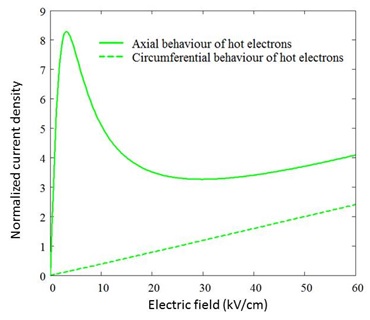
Figure 1: A plot of normalized current density versus electric field for a ($4,1$) chiral CNT, $\eta=1.7\times 10^{-8}$, $v=1\mathrm{THz}$ and $T=287.5\ \mathrm{K}$

The normalized axial current density of ($4$, $1$) chiral CNT exhibits a linear monotonic dependence on the applied electric field at lower field (i.e. the region of ohmic conductivity). As the electric field increases, the axial current density increases and reaches a maximum at about $3.5\ \mathrm{kV/cm}$, and drops off, experiencing a negative differential conductivity (NDC) up to about $25\ \mathrm{kV/cm}$ as shown in figure 1. The NDC is due to the increase in the collision rate of the energetic electrons with the lattice that induces large amplitude oscillation in the lattice, which in-turn increases the scattering rate that leads to the decrease in the current [24]. When the electric field exceeds about $25\ \mathrm{kV/cm}$, we once again observe an increase in normalized axial current density of chiral carbon nanotube. Hence there is switch from NDC to PDC when electric field value of about $25\ \mathrm{kV/cm}$ is exceeded. This phenomena also occurs when there is an impact ionization. This has been studied in superlattices [28] The physical mechanism behind the switch from NDC to PDC has been explained in  [24, 25] The normalized circumferential current density of ($4$, $1$) chiral CNT exhibits a linear monotonic dependence on the applied electric field as up to $60\ \mathrm{kV/cm}$ as shown in figure $1$. Especially from $0$ to about $10\ \mathrm{kV/cm}$, conductivity is mainly axially and hence circumferential conductivity is negligible or can be ignored. This is due to an extremely high length-to-diameter aspect ratio of CNTs up to $132000000:1$ which is significantly larger than any other material [26]. Hence CNTs are quasi-$1$D carbon materials. In figure $2$, we only display the behaviour of the normalized axial current density as a function of the electric field for ($4$, $1$) chiral CNT stimulated axially with the hot electrons, represented by the non-equilibrium parameter $\eta$. In figure $2$, there is a switch from NDC to PDC in a ($4$, $1$) chiral CNT when $\eta=0.9\times 10^{-8}$ near $35\ \mathrm{kV/cm}$. As we increase the rate of hot electrons injection represented by non-equilibrium parameter $\eta$ from $0.9\times 10^{-8}$ to $3.0\times 10^{-8}$ chiral CNT, the behviour of hot electrons change leading to an increase in differential conductivity $|{\partial J\over\partial E}|$ as well as the peak normalized axial current density as shown in figure $2$

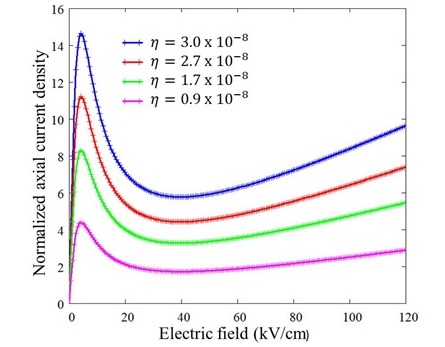
Figure 2: Aplot for Normalized axial current density versus Electric field $\mathrm{(kV/cm)}$ as non-equilibrium parameter $\eta$ increases, $\mathrm{v=1THz}$ and $\mathrm{T=287.5K}$

To put the above observations in perspective, we display in figure $3$ a 3-dimensional behaviour of the normalized axial current density $(Ja)$ as a function of the electric field $(E)$ and non-equilibrium parameter $(\eta)$. The differential conductivity and the peak of the current density are at the lowest values when the non-equilibruim parameter $\eta=0$. As non-equilibrium parameter $\eta$ increases from 0 to $30\times 10^{-9}$, both differential conductivity and peak current density increase. Therefore, the behaviour of hot electrons under the influence of dc field in chiral carbon nanotube leads to a switch from NDC to PDC, differential conductivity and the peak normalized current density increase.

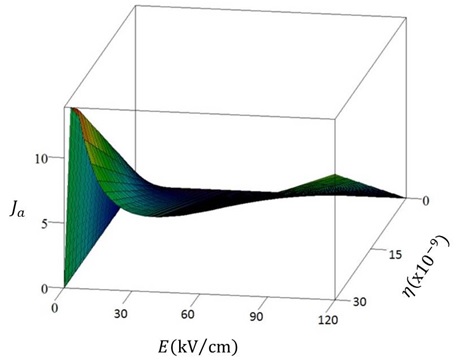
Figure 3: A 3D plot of normalized axial current density $(Ja)$ versus electric field $(E)$ and non-equilibrium parameter $(\eta)$

In figure $4$, we display the behaviour of the normalized axial current density as a function of the electric field for the achiral CNTs stimulated axially with the hot electrons, represented by the non-equilibrium parameter $\eta=1.7\times 10^{-8}$ as in  [24]

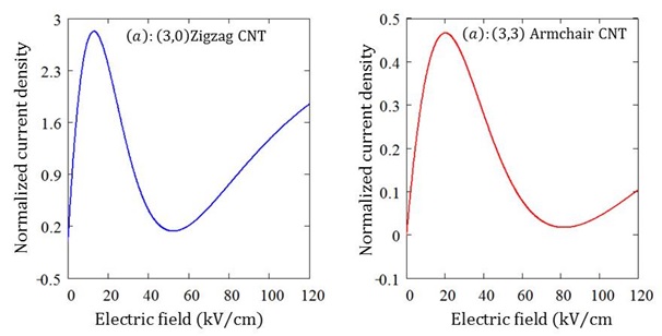
Figure 4: A plot of normalized current density versus electric field for (a) ($3$, $0$) zigzag CNT and (b) ($3$, $3$) armchair both stimulated axially with the hot electrons, represented by the nonequilibrium parameter $\eta=1.7\times 10^{-8}$ as in [24]

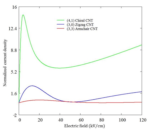
Figure 5: A plot of the normalized axial current density versus electric field for ($3$, $0$) zigzag CNT, ($3$, $3$) CNT [24] and ($4$,$1$) CNT stimulated axially with the hot electrons, represented by the non-equilibrium parameter $\eta=1.7\times 10^{-8}$

We generally observed in figure $5$ that with axial injection of hot electrons in ($4$, $1$) chiral CNT, ($3$, $0$) zigzag CNT and ($3$, $3$) armchair CNT under the influence of dc field, there is the desirable effect of a switch from NDC to PDC characteristics. Thus, the most important tough problem for NDC region which is the space charge instabilities can be suppressed due to the switch from the NDC behaviour to the PDC behaviour predicting a potential generation of terahertz radiations [25] which have enormous promising applications in very different areas of science and technology [27]. However, there are some differences such as differential conductivity, peak normalized current density, critical dc field beyond which NDC characteristics occurs and finally the value of dc field above which there is a desirable switch of NDC to PDC. First and foremost, the differential conductivity $|{\partial J\over\partial E}|$ of ($4$, $1$) chiral CNT is the highest, ($3$, $3$) armchair CNT is the least while that of ($3$, $0$) zigzag CNT is between the two. Also in figures $4$ and $5$, the peak normalized current density for ($4$, $1$) chiral CNT, ($3$, $3$) zigzag CNT and ($3$, $3$) CNT are about $14.20$, $2.70$ and $0.46$ respectively. Hence ($4$, $1$) chiral CNT is having the highest peak normalized current density follow by ($3$, $0$) zigzag CNT whereas ($3$, $3$) CNT is the least. Furthermore, the critical dc fields that should be exceeded before NDC are observed in ($4$, $1$) chiral CNT, ($3$, $0$) zigzag CNT and ($3$, $3$) armchair CNT are about $6\ \mathrm{kV/cm}$, $12\ \mathrm{kV/cm}$ and $20\ \mathrm{kV/cm}$ respectively in figures $4$ and $5$. Finally, if the rate of axial injection of hot electrons represented by non-equilibrium parameter $\eta=1.7\times 10^{-8}$, there is a switch from NDC to PDC near $35\ \mathrm{kV/cm}$, $50\ \mathrm{kV/cm}$, $75\ \mathrm{kV/cm}$ for ($4$, $1$) chiral CNT, ($3$, $0$) zigzag CNT and ($3$, $3$) armchair CNT respectively.

3 Conclusion

In summary, behaviour of hot electrons under the influence of dc field in chiral carbon nanotubes have been demonstrated theoretically by adopting semiclassically approximation approach in solving Boltzmann transport equation. It leads to changes in the nature of the dc differential conductivity by switching from an NDC characteristics to PDC characteristics due to the hot electrons injection. Thus, domain instability can be suppressed, suggesting a potential generation of terahertz radiations with enormous promising applications in very different areas of technology, industry and research. Unlike achiral CNTs, a potential generation of terahertz radiations in chiral counterpart can take place at lower dc field which stems from our research findings that the switch from NDC to PDC occurs at relatively low dc field.

References

- [1] Ravi Kumar Goel and Annima Panwar, International Journal of Latest Research in Science and Technology, l ,155(2012)
- [2] R. Saito, G. Dresselhaus, M.S. Dresselhaus, Physical Properties of Carbon Nanotubes (London and Imperial College Press, 1998)
- [3] M.D. Dresselhaus, G. Dresselhaus, P. Avouris, Carbon Nanotubes: Synthesis and Structure and Properties and Applications (Springer-Verlag, Berlin, 2001)
- [4] H. Dai, Surf. Sci. 500, 218 (2002)
- [5] M. Pudlak , R. Pincak and V.A. Osipov, Journal of Physics: Conference Series, 129, 012011 (2008)
- [6] K. Liu, M. Burghard, S. Roth, Appl. Phys Lett. 75, 2494 (1999)
- [7] C. Dekker, Phys. Today 52, 22 (1999).
- [8] P. L. McEuen, M. S. Fuhrer and H. K. Park, IEEE Trans. Nanotechnology 1, 78 (2003).
- [9] A. Javey et al., Nature Materials 1, 241 (2002).
- [10] A. Javey, J. Guo, Q. Wang, M. Lundstrom and H. J. Dai, Nature, 424, 654 (2003).
- [11] A. Javey et al., Nano Lett. 4, 1319 (2004).
- [12] T. Durkop, S. A. Getty, E. Cobas and M. S. Fuhrer, Nano Lett. 4, 35 (2004).
- [13] Y. M. Lin et al., IEEE Elec. Dev. Lett. 26, 823 (2005).
- [14] N. Balkan, Hot Electrons in Semiconductors, Physics and Device, Clarendon Press, Oxford (1998)
- [15] Serge Luryi and Alexander Kastalsky, Physica B 134 453(1985)
- [16] A.S. Maksimenko, G.Ya. Slepyan, Phys. Rev. Lett. 84, 362 (2000)
- [17] D.A. Ryndyk, N.V. Demarina, J. Keller, E. Schomburg, Phys. Rev. B 67, 033305 (2003)
- [18] G. Ya Slepyan, S.A. Maksimenko, A. Lakhtakia, O. M. Yevtushenko, A. V. Gusakov, Phys. Rev. B 57,9485 (1998)
- [19] O. M. Yevtushenko, Phys. Rev. Lett., 79, 1102 (1997)
- [20] H. Kajiura et al., Carbon, 43, 1317 (2005).
- [21] I. M. Lifshits, M. Azbel, and M. I. Kaganov,Electron Theory of Metals Consultants Bureau, New York, 1973!.
- [22] Mensah, N. G., G. K. Nkrumah-Buandoh, S. Y. Mensah, F. K. A. Allotey, and Anthony K. Twum. Thermoelectric figure of merit of chiral carbon nanotube. Abdus Salam International Centre for Theoretical Physics, Trieste (Italy), 2005.
- [23] Dass, Devi, Rakesh Prasher, and Rakesh Vaid. ”Analytical study of unit cell and molecular structures of single walled carbon nanotubes.” International Journal of Computational Engineering Research 2 (2012): 1447-1457.
- [24] Amekpewu , Matthew, Sulemana S. Abukari, Kofi W. Adu, Samuel Y. Mensah, and Natalia G. Mensah. ”Effect of hot electrons on the electrical conductivity of carbon nanotubes under the influence of applied dc field.” The European Physical Journal B 88, no. 2 (2015): 1-6.
- [25] Amekpewu, M., S. Y. Mensah, R. Musah, N. G. Mensah, S. S. Abukari, and K. A. Dompreh. ”Hot electrons injection in carbon nanotubes under the influence of quasi-static ac-field.” arXiv preprint arXiv:1510.06844 (2015)
- [26] X. Wang, Q. Li, J. Xie, Z. Jin, J. Wang, Y. Li, K. Jiang, and S. Fan. Fabrication of Ultralong and Electrically Uniform Single-Walled Carbon Nanotubes on Clean Substrates. Nano Letters, 9: 3137-3141, 2009
- [27] Amekpewu, M., S. Y. Mensah, R. Musah, N. G. Mensah, S. S. Abukari, and K. A. Dompreh. ”High Frequency Conductivity of Hot Electrons in Carbon Nanotubes.” arXiv preprint arXiv:1507.04583 (2015).
- [28] S. Y. Mensah, F. K. A. Allotey, and A. Clement. ”Effect of ionization of impurity centres by electric field on the conductivity of superlattice.” Superlattices and microstructures 19.2 (1996): 151-158.