Iterative regularization via dual diagonal descent

Abstract

In the context of linear inverse problems, we propose and study a general iterative regularization method allowing to consider large classes of regularizers and data-fit terms. The algorithm we propose is based on a primal-dual diagonal descent method. Our analysis establishes convergence as well as stability results. Theoretical findings are complemented with numerical experiments showing state of the art performances.

Keywords: Splitting methods, Dual problem, Diagonal methods, Iterative regularization, Early stopping

Mathematics Subject Classifications (2010): 90C25, 49N45, 49N15, 68U10, 90C06

1 Introduction

Many applied problems in science and engineering can be modeled as noisy inverse problems. This is true in particular for many problems in image processing, such as image denoising, image deblurring, image segmentation, or inpainting. Tackling these problems requires to deal with their possible ill-posedeness [50] and to devise efficient numerical procedures to quickly and accurately compute a solution.

Tikhonov regularization is a classical approach to restore well-posedness [47]. A stable solution is defined by the minimization of an objective function being the sum of two terms: a data-fit term and a regularizer ensuring stability. From a numerical perspective, first order methods have recently become popular to solve the corresponding optimization problem [37]. Indeed, simplicity and low iteration cost make these methods especially suitable in large scale applications.

In practice, finding the best Tikhonov regularized solution requires specifying a regularization parameter determining the trade-off between data-fit and stability. Discrepancy principles [50], SURE [70, 45], and cross-validation [71] are some of the methods used to this purpose. An observation important for our work is that, from a numerical perspective, choosing the regularization parameter for Tikhonov regularization typically requires solving not one, but several optimization problems, i.e. one for each regularization parameter to be tried. Clearly, this can dramatically increase the computational costs to find a good solution, and the question of how to keep accuracy while ensuring better numerical complexity is a main motivation for our study.

In this paper, we depart from Tikhonov regularization and consider iterative regularization approaches [12]. The latter are classical regularization techniques based on the observation that stopping an iterative procedure corresponding to the minimization of an empirical objective has a self-regularizing property [50]. Crucially, the number of iterations becomes the regularization parameter, and hence controls at the same time the stability of the solution as well as the computational complexity of the method. This property makes parameter tuning numerically efficient and iterative regularization an alternative to Tikhonov regularization, which potentially alleviates the aforementioned drawbacks. Indeed, an advantage of iterative regularization strategies is that they are developed in conjunction with the optimization algorithm, which is tailored to the structure of the problem of interest.

Iterative regularization methods are classical both in linear [50] and non linear inverse problems [12, 53], for quadratic data-fit term and quadratic regularizers. Extensions to more general regularizers have been considered in recent works [10, 26, 27, 21]. However, we are not aware of iterative regularization methods that allow considering more general data-fit terms. Indeed, while this is easily done in Tikhonov regularization, how to do the same in iterative regularization is less clear and our study provides an answer.

Our starting point is viewing the inverse problem as a hierarchical optimization problem defined by the regularizer and the data-fit term. The latter can belong to wide classes of convex, but possibly non-smooth functionals. To solve such an optimization problem we combine duality techniques [36] with a diagonal approach [11]. As a result, we obtain a primal-dual method, given by a diagonal forward-backward algorithm on the dual problem. The algorithm thus obtained is simple and easy to implement. Our main result proves convergence in the noiseless case, and is an optimization result interesting in its own right. Combining this result with a stability analysis allows to derive iterative regularization properties of the method. Our theoretical analysis is complemented with numerical results comparing the proposed method with Tikhonov regularization on various imaging problems. The obtained results show that our approach is competitive in terms of accuracy and often outperforming Tikhonov regularization from a numerical perspective. To the best of our knowledge, our analysis is the first study on iterative regularization methods for general data-fit terms and hence it is a step towards broadening the applicability and practical impact of these techniques.

The rest of the paper is organized as follows. In Section 2 we collect some technical definitions and results needed in the rest of the paper, whereas in Section 3 we recall the basic ideas in inverse problems and regularization theory. In Section 4 we introduce the algorithm we propose in this paper and present in Section 5 its regularization properties, which constitutes our main results. The theoretical analysis of the (3-D) method is made in Sections 6 and 7, while Section 8 contains its numerical study. The Appendix contains the proof of some auxiliary and technical results.

2 Background and notation

We give here some mathematical background needed in the paper. We refer to [14, 65] for an account of the main results in convex analysis.

Since our algorithm will essentially rely on duality arguments, we first introduce the notion of (Fenchel) conjugate. Let $H$ be a Hilbert space, $2^{H}$ its power set, and $f:H\longrightarrow[-\infty,+\infty]$. Its Fenchel conjugate $f^{*}:H\longrightarrow[-\infty,+\infty]$ is

$$(\forall x\in H)\quad f^{*}(x):=\sup_{x^{\prime}\in H}\left\{\langle x^{\prime},x\rangle-f(x^{\prime})\right\}.$$

We say that $f$ is coercive if $\lim_{\|x\|\to+\infty}f(x)=+\infty$. We denote by $\Gamma_{0}(H)$ the set of proper, convex and lower semi-continuous functions from $H$ to $]-\infty,+\infty]$. Let $\sigma\in\left]0,+\infty\right[$. We say that $f\in\Gamma_{0}(H)$ is $\sigma$-strongly convex if $f-{\sigma}\|\cdot\|^{2}/2\in\Gamma_{0}(H)$. The Fenchel conjugate of a $\sigma$-strongly convex function is differentiable, with a $\sigma^{-1}$-Lipschitz continuous gradient [14, Theorem 18.15]. We recall that the subdifferential of $f\in\Gamma_{0}(H)$ is the operator $\partial f:H\rightarrow 2^{H}$ defined by, for every $x\in H$,

$$x^{*}\in\partial f(x)\Leftrightarrow(\forall x^{\prime}\in H)\ \ \ f(x^{\prime})-f(x)-\langle x^{*},x^{\prime}-x\rangle\geq 0.$$

If $f$ is Fréchet differentiable at $x\in H$, then $\partial f(x)=\{\nabla f(x)\}$. The subdifferential also enjoys a symmetry property with respect to the Fenchel conjugation [14, Theorem 16.23]:

$$(\forall(x,x^{*})\in H^{2})\quad x^{*}\in\partial f(x)\Leftrightarrow x\in\partial f^{*}(x^{*}).$$

Given two functions $f,g\in\Gamma_{0}(H)$, their infimal convolution (or inf-convolution) is the function $f\#g$ in $\Gamma_{0}(H)$ defined by

$$(\forall x\in H)\quad(f\#g)(x):=\inf\limits_{x^{\prime}\in H}\left\{f(x^{\prime})+g(x-x^{\prime})\right\}.$$

The Fenchel conjugate of the infimal convolution of two functions can be simply computed by the following rule [14, Proposition 13.21(i)]

$$(f\#g)^{*}=f^{*}+g^{*}.$$ (2.1)

We also recall the notion of proximity operator, which is a key tool to define the algorithm we study. The proximity operator of $f\in\Gamma_{0}(H)$ is the operator $\mbox{\rm prox}_{f}:H\longrightarrow H$ defined by, for every $x\in H$,

$$\mbox{\rm prox}_{f}(x)=\underset{x^{\prime}\in H}{\operatorname{argmin}}\left\{f(x^{\prime})+\frac{1}{2}\|x^{\prime}-x\|^{2}\right\}.$$ (2.2)

The proximity operator is particularly relevant when computing the gradient of the conjugate of a strongly convex function.

Lemma 2.1

Let $H_{1},H_{2}$ be Hilbert spaces. Let $J\in\Gamma_{0}(H_{2})$, $\sigma\in\left]0,+\infty\right[$, $x^{\prime}\in H_{1}$, and $W\colon H_{1}\to H_{2}$ be a linear orthogonal operator. Let $f\in\Gamma_{0}(H_{1})$ be the function defined by $f(x)=J(Wx)+{\sigma}\|x-x^{\prime}\|^{2}/2.$ Then,

$$(\forall x\in H_{1})\quad\nabla f^{*}(x)=W^{*}\mbox{\rm prox}_{\sigma^{-1}J}(Wx^{\prime}+\sigma^{-1}Wx).$$

The proof is postponed to Appendix 10.1.

We end this section by introducing the notion of conditioning [75, 77, 79], which is a common tool in the optimization and regularization literature [60, 19], and will be required later for the data-fit function.

Definition 2.2

Let $f\in\Gamma_{0}(H)$ having a unique minimizer $x_{0}\in H$. The function $f$ is said to be well conditioned if there exists a positive even function $m\in\Gamma_{0}(\mathbb{R})$ such that, for every $t\in\mathbb{R}$, $m(t)=0\implies t=0$, and

$$(\forall x\in H)\quad m\left(\|x-x_{0}\|\right)\leq f(x)-f(x_{0}).$$ (2.3)

In that case, $m$ is called a conditioning modulus (or growth modulus) for $f$. Let $p\in\left[1,+\infty\right[$. We say that $f$ is $p$-well conditioned, if there exists $(\varepsilon,\gamma)\in\left(\left]0,+\infty\right[\right)^{2}$ such that

$$\left(\forall t\in\left]-\varepsilon,\varepsilon\right[\right)\quad m(t)\geq\frac{\gamma}{p}|t|^{p}$$ (2.4)

Notation.

We adopt the following standard notation: $\mathbb{R}_{+}=\left[0,+\infty\right[$, $\mathbb{R}_{++}=\left]0,+\infty\right[$, $\mathbb{R}^{d}_{++}=\left]0,+\infty\right[^{d}$, $\mathbb{N}^{*}=\mathbb{N}\setminus\{0\}$. The identity operator from a set to itself is denoted by $\operatorname{Id}$. Given $C$ a subset of a topological space, $\mathrm{int}C$ denotes the interior of $C$. The set of minimizers of a function $f$ is denoted by $\operatorname{argmin}f$, and its domain is noted $\mathop{\mathrm{missing}}{\rm dom}f$. The range of a linear operator $A:H_{1}\rightarrow H_{2}$ will be denoted by $\operatorname{Im}A$, and its norm is denoted by $\|A\|$. The norms in the considered Hilbert spaces are always denoted by $\|\cdot\|$.

3 Background: inverse problems and regularization

In this section, we recall basic notions in inverse problems theory and introduce Tikhonov and iterative regularization.

3.1 Linear inverse problems

Let $X$ and $Y$ be Hilbert spaces. Given $\bar{y}\in Y$ and a bounded linear operator $A:X\longrightarrow Y$ the corresponding inverse problem is to find ${\bar{x}}\in X$ satisfying

$${\bar{y}}=A{\bar{x}}.$$ (3.1)

For example, in denoising $A=Id$ and in deblurring $A$ is an integral operator for suitable kernel. In general, the above problem is ill-posed, in the sense that a solution might not exist, might not be unique, or might not depend continuously to the data $\bar{y}$ [50]. The first step towards restoring well-posedness is then to introduce a notion of generalized solution. This latter definition hinges on the choice of a regularizer, that is a functional $R\in\Gamma_{0}(X)$ and a data-fit function $D:Y^{2}\longrightarrow\mathbb{R}\cup\{+\infty\}$. A generalized solution $x^{\dagger}\in X$ is then defined as a solution of the problem

$$\text{minimize}\ \left\{R(x)\ \left|\ x\in\operatorname{argmin}_{x^{\prime}\in X}D(Ax^{\prime},\bar{y})\right\}\right.. P$$ ()

Consider the following classical example to illustrate the above definition.

Example 3.1 (Moore-Penrose solution)

Let $R(x)=\|x\|$ and $D(Ax,y)=\|Ax-y\|^{2}$ for all $x\in X$. Then, under mild assumptions, there exists a unique generalized solution to ($P$) which is the Moore-Penrose solution $x^{\dagger}=A^{\dagger}\bar{y}$, where $A^{\dagger}$ is the pseudo-inverse of $A$ [50].

We add two comments. First, note that there might be more than one generalized solution, however in the following we will restore uniqueness of $x^{\dagger}$ by assuming $R$ to be strongly convex. Second, as we discuss next, in general $x^{\dagger}$ might not depend continuously on $\bar{y}$, as it is clear from the Example 3.1. This last observation is crucial, since in practice only a noisy datum is available. Ensuring continuity, hence stability, to noisy data is the main motivation of regularization techniques described in the next section. We first add a few further examples of regularizers and data-fit functions, and one remark.

Example 3.2 (Regularizers)

A choice of regularizer popular in image processing is the $\ell^{1}$-norm of the coefficients of $x\in X$ with respect to an orthonormal basis, or a more general dictionary, e.g. a frame. Indeed, this regularizer can be shown to correspond to a sparsity prior assumption on the solution [61]. Another popular choice of regularizer is the total variation [68], due to its ability to preserve edges. Other possibilities are total generalized variation [23], or infimal convolutions between total variation and higher order derivatives [32]. Yet another possibility is to consider a Huber norm of the gradient, instead of the $L^{1}$ norm [33]. We refer to [56] for additional references.

We next discuss several examples of data-fit functions. Flexibility in the choice of the latter is a key aspect for our study.

Example 3.3 (Data-fit function)

As mentioned above, a classical choice for the data-fit function is the $\ell^{2}$ norm:

$$(\forall(u,y)\in Y^{2})\quad D(u;y)=\|u-y\|^{2}/2.$$

We list a few further examples.

• the $\ell^{1}$-norm in $\mathbb{R}^{d}$,

  $$(\forall(u,y)\in\mathbb{R}^{d}\times\mathbb{R}^{d})\quad D(u;y)=\|u-y\|_{1};$$

• the Kullback-Leibler divergence, defined , for every $y\in\mathbb{R}^{d}$, as $D(u;y):=\mathrm{KL}(y,u)=\sum_{i=1}^{d}\mathrm{kl}(y_{i},u_{i})$, where

  $$\mathrm{kl}(y_{i},u_{i})=\begin{cases}\displaystyle\sum_{{i=1}}^{d}y_{i}\log\frac{y_{i}}{u_{i}}-y_{i}+u_{i}&\text{if }(y_{i},u_{i})\in\left]0,+\infty\right[^{2}\\[8.61108pt] +\infty&\text{otherwise;}\end{cases}$$

• the weighted sum of $L^{1}$ and $L^{2}$ norms in $\mathbb{R}^{d}$ [52],

  $$(\forall(u,y)\in\mathbb{R}^{d}\times\mathbb{R}^{d})\quad D(u;y)=\|u-y\|_{1}+\frac{\sigma}{2}\|u-y\|^{2},$$

  for some $\sigma\in\left]0,+\infty\right[$;

• the Huber data-fit function [30] in $\mathbb{R}^{d}$. Let $\sigma\in\mathbb{R}_{++}$ and the Huber function be $h_{\sigma}\colon\mathbb{R}\to\mathbb{R}_{+}$,

  $$(\forall t\in\mathbb{R})\quad h_{\sigma}(t)=\begin{cases}\frac{1}{2\sigma}t^{2}&\text{ if }|t|\leq\sigma\\ |t|-\frac{\sigma}{2}&\text{ otherwise.}\end{cases}$$ (3.2)

  Then the corresponding data-fit function can be formulated as, $(\forall(u,y)\in\mathbb{R}^{d}\times\mathbb{R}^{d})$,

  $$D(u;y)=H_{\sigma}(u-y):=\sum\limits_{i=1}^{d}h_{\sigma}(u_{i}-y_{i}).$$

Both the choice of the regularizer and the data-fit function reflect some prior information about the problem at hand. This latter observation can be further developed taking a probabilistic (Bayesian) perspective, as we recall in the next remark.

Remark 3.4 (Bayesian interpretation)

In a Bayesian framework, the choice of regularizers and data-fit functions can be related to the choice of a prior distribution on the solution and a noise model with a corresponding likelihood. In particular, for the data fit functions it can be seen that the quadratic norm is related to Gaussian noise and moreover,

• the $L^{1}$-norm is related to impulse noise, e.g. salt and pepper or random-valued impulse noise [63],

• the Kullback-Leibler divergence is related to Poisson noise [57],

• the weighted sum of $L^{1}$ and $L^{2}$ norms is related to mixed Gaussian and impulse noise [52],

• and the Huber data-fit function [30] is related to the mixed Gaussian and impulse noise.

3.2 Tikhonov and iterative regularization

The basic idea of regularization is to approximate a generalized solution $x^{\dagger}$ of ($P$) with a family of solutions having better stability properties. More precisely, given a pair $(A,\bar{y})$, a regularization method defines a sequence $(x_{\lambda})_{\lambda\in\Lambda}\in X$, where $\Lambda=]0,+\infty[$, or $\Lambda=\mathbb{N}$. The idea is that the so called regularization parameter $\lambda$ controls the accuracy with which $x_{\lambda}$ approximates $x^{\dagger}$. Indeed, the first basic regularization property is to require

$$x_{\lambda}\to x^{\dagger},\text{ as }\lambda\to 0,$$ (3.3)

(or as $\lambda\to+\infty$ when $\Lambda=\mathbb{N}$). The second basic property of a regularization method is stability. Given $\hat{y}$ a noisy version of the exact datum $\bar{y}$, this latter property can be seen as the requirement for the sequence $(\hat{x}_{\lambda})_{\lambda\in\Lambda}\in X$, corresponding to the regularization method applied to $(A,\hat{y})$, to be sufficiently close to $(x_{\lambda})_{\lambda\in\Lambda}\in X$. This latter property, together with the regularization property, allows to show that $\hat{x}_{\lambda}$ is a good approximation to $x^{\dagger}$ – at least provided a suitable regularization parameter choice $\lambda\in\Lambda$. We refer to [50] for further details and illustrate the above definitions with two specific examples of regularization operators.

Tikhonov regularization.

In the setting of Example 3.1, Tikhonov regularization is defined by the following minimization problem

$$x_{\lambda}=\underset{\begin{subarray}{c}{x\in X}\end{subarray}}{\text{\rm minimize}}\;\;\|x\|^{2}+\frac{1}{\lambda}\|Ax-y\|^{2}.$$

The above approach easily extends to more general regularizers/data-fit terms considering

$$\quad x_{\lambda}=\underset{\begin{subarray}{c}{x\in X}\end{subarray}}{\text{\rm minimize}}\;\;R(x)+\frac{1}{\lambda}D(Ax,y). P_{\lambda}$$ ()

From the above definition it is clear that Tikhonov regularization requires to solve an optimization problem, for each value of the regularization parameter $\lambda$. For large scale applications, or if the problem is non-linear, solving $(P_{\lambda})$ exactly is not possible, so only an approximation of $x_{\lambda}$ can be considered. While a variety of techniques can be used to this purpose, iterative methods, and in particular those based on first order methods, are particularly favored. Broadly speaking, for each regularization parameter $\lambda\in\Lambda\subset]0,+\infty[$, an iterative optimization method is defined by a sequence

$$x_{0,\lambda}\in X,\ x_{n+1,\lambda}=\text{Algorithm}(x_{n,\lambda};\lambda;y),$$ (3.4)

in such a way that $x_{n,\lambda}$ tends to $x_{\lambda}$ as $n$ grows. It is then clear that, as mentioned in the introduction, the need to select a regularization parameter can have a dramatic effect from a numerical perspective. Indeed, in practice $\Lambda$ is a finite set $\Lambda_{N}\subset]0,+\infty[$, and an optimization problem needs to be solved for each regularization parameter $\lambda\in\Lambda_{N}$. If $N$ is the cardinality of the set $\Lambda_{N}$, the numerical complexity of the iteration (3.4) is now multiplied by $N$.

The question of deriving alternative regularization techniques tackling directly non-linearity and large scale issues, and having better complexity, is then of both theoretical and practical relevance. As mentioned next, iterative regularization provides one such alternative.

Iterative regularization.

Iterative regularization is typically derived considering an iterative optimization procedure to solve directly problem ($P$) (rather than ($P_{\lambda}$)),

$$x_{0}\in X,\ x_{n+1}=\text{Algorithm}(x_{n};y).$$ (3.5)

For instance, in the setting of Example 3.1, a classical iterative regularization method is the Landweber method [50] defined by the iteration

$$x_{0}\in X,\ x_{n+1}=x_{n}-\tau A^{*}(Ax-y),$$

where $\tau\in\left]0,2\|A\|^{-2}\right[$ is a stepsize. Note that for iterative regularization methods, the regularization parameter is the number of iterations. In this setting, the regularization property (3.3) reduces to the convergence of the iteration to $x^{\dagger}$ when (3.5) is applied with $y=\bar{y}$. Stability, when iteration (3.5) is applied to noisy data, is ensured by defining a regularization parameter choice, which in this case is a stopping criterion.

When compared to Tikhonov regularization, the advantage of iterative regularization is mostly numerical. Computing solutions corresponding to different regularization parameters is straightforward, since the latter is simply the number of iterations. In practice, this property often turns into dramatic computational speed-ups while performing regularization parameter tuning.

A main motivation for this work is the observation that, differently from Tikhonov regularization, how to design iterative regularization for general regularizers and data-fit terms is not as clear. Iterative regularization method that allow to consider more general regularizers are known in the literature, but are typically restricted to quadratic data-fit functions. In practice this latter choice can be limiting, since considering different data-fit functions is often crucial. However, we are not aware of studies considering iterative regularization for general classes of error functions. The results we describe next are a step towards filling this gap.

4 The Diagonal Dual Descent (3-D) method

In this section, we describe the iterative algorithm we propose and analyze in the rest of the paper. We begin by an informal description introducing some basic ideas, before providing a more detailed discussion.

4.1 Diagonal algorithms

We will consider an iterative optimization method based on a diagonal principle. The classic idea [11] is to combine an optimization algorithm, with a sequence of approximations of the given problem ($P$), changing eventually the approximation at each step of the algorithm. In our setting, this corresponds to an algorithm as in (3.4) where the parameter $\lambda$ can be updated at each iteration,

$$x_{0}\in X,\ x_{n+1}:=\text{Algorithm}(x_{n};\lambda_{n};y),\ \lambda_{n}\to 0.$$ (4.1)

Roughly speaking, we allow the algorithm to “switch” between penalized problems corresponding to different values of $\lambda$. As briefly recalled previously, for iterative regularization methods, the number of iterations, and thus here the sequence $(\lambda_{n})_{n\in\mathbb{N}}$, controls the accuracy with which $x_{n}$ approaches $x^{\dagger}$.

We will first show that the basic regularization property holds, namely that in the noiseless case $x_{n}\to x^{\dagger}$, as $n\to+\infty$, provided that $\lambda_{n}\to 0$. Then, we will prove stability with respect to noise. Combining this latter property with the regularization one will allow us to derive a suitable stopping rule and to build a stable approximation of $x^{\dagger}$. In particular, in the presence of noise, the stopping rule will impose termination of the iterative procedure before $\lambda_{n}$ reaches $0$, preventing numerical instabilities. We now illustrate the diagonal principle in the setting of Example 3.1.

Example 4.1

(Diagonal Landweber algorithm) In the setting of Example 3.1, a basic diagonal algorithm is the diagonal Landweber algorithm

$$\begin{array}[]{|l}{x}_{0}\in X,\ \lambda_{n}\to 0,\ \tau>0\text{ is a stepsize},\\ {x}_{n+1}={x}_{n}-\tau A^{*}(A{x}_{n}-{y})-\tau\lambda_{n}{x}_{n}.\end{array}$$ (4.2)

The above iteration can be seen as the gradient descent method applied to ($P_{\lambda}$), for $R=\frac{1}{2}\|\cdot\|^{2}$ and $D(\cdot;y)=\frac{1}{2}\|\cdot-{y}\|^{2}$, and especially considering $\lambda$ to change at each iteration. The above iteration has been mainly studied for nonlinear inverse problems, and is known under several names: modified Landweber iteration [69], iteratively regularized Landweber iteration [53], iteratively regularized gradient method [12], or Tikhonov-Gradient method [66]. In Figure 1, we illustrate the difference between the diagonal Landweber algorithm and the classic Tikhonov method.

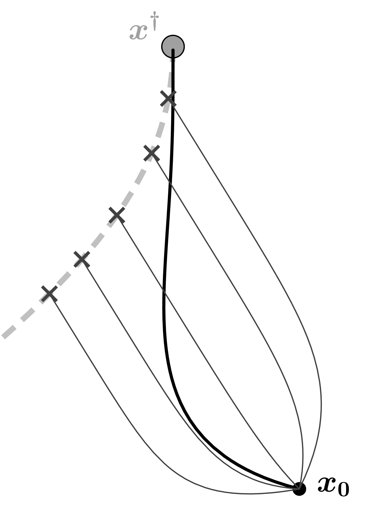
Figure 1: Thick dotted line: Tikhonov regularization path $\{x_{\lambda}\}_{\lambda>0}$. Thin plain lines: Gradient Descent solving $(P_{\lambda})$ for $\lambda\in\{1,0.75,0.5,0.25,0.1\}$, starting from $x_{0}$. Thick plain line: Diagonal Landweber algorithm, with $\lambda_{n}=(n+1)^{-1}$. Here $A=[(1,1)^{T},(1,0)^{T}]$ and $y=(2,1)^{T}$.

It is interesting to relate diagonal methods to “warm-restart”, a heuristic commonly used to speed up the computations of Tikhonov regularized solutions for different regularization parameter values [17].

Example 4.2

(Warm restart) Warm restart, or continuation method, is a popular heuristic used to approximately follow the path $\{x_{\lambda}\,\colon\,\lambda\in\Lambda\}$ of solutions of problem ($P_{\lambda}$). The method is based on considering a sequence of problems $(P_{\lambda_{i}})_{i\in\mathbb{N}}$ for a decreasing family of parameters $(\lambda_{i})_{i\in\mathbb{N}}$ in $\mathbb{R}_{++}$. Then, the solutions corresponding to larger values of $\lambda_{i}$ are computed first and used to initialize – “warm” start – the next problem. The rationale behind the method, is the empirical observation that solving ($P_{\lambda}$) with a first-order method as in (3.4) is faster if $\lambda$ is large [51]. It is easy to see that this continuation strategy generates a sequence $(x_{n})_{n\in\mathbb{N}}$ which corresponds to the diagonal algorithm (4.1), for a piecewise constant decreasing sequence $(\lambda_{n})_{n\in\mathbb{N}}$. The warm restart principle is illustrated in Figure 2.

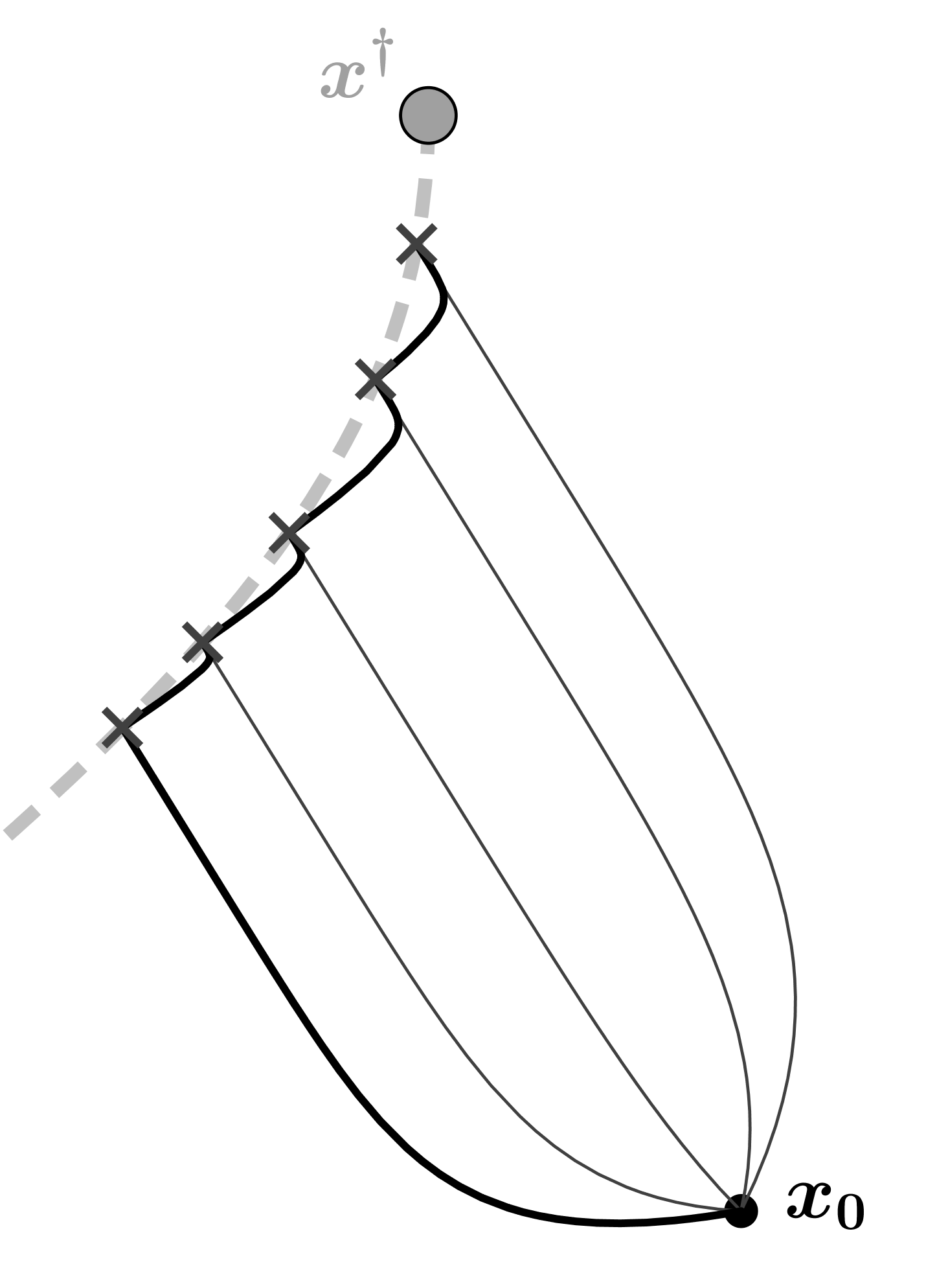
Figure 2: Exact same setting than for Figure 1, but here $\lambda_{n}$ is constant by parts, taking successively its values in $\{1,0.75,0.5,0.25,0.1\}$.

In the optimization setting, the literature on diagonal methods is vast. Diagonal procedures as in (4.1) have been the object of various studies since the 70’s [22, 54, 62, 55], considering various algorithms coupled with a large class of penalization methods, such as Tikhonov penalization, exponential barrier methods, interior methods, or more general principles. More precisely, diagonal versions of the proximal algorithm have been considered in [54, 55, 9, 1, 72, 42, 2, 29], the diagonal gradient method has been studied in [64], and the diagonal projected gradient method in [22, 62]. More recently, a diagonal version of the forward-backward algorithm has been investigated in [58, 59, 7, 43], see also [76, Section 17.3.2]. The above papers are concerned with convergence of the considered optimization criterion, corresponding to the regularization property for noiseless data in inverse problems. Stability and early stopping results are known only for the diagonal Landweber method [69, 66, 12, 53].

A main novelty of our work is considering a dual diagonal approach, since the diagonal methods studied in the literature are essentially primal. These latter approaches are well suited if the data-fit function $x\mapsto D(Ax;y)$ is “simple”, in the sense that either the proximity operator of $x\mapsto D(Ax;y)$ is easy to compute, or $D$ is smooth. However, these properties might not be satisfied by the data-fit functions of interest, see Example 3.3. In particular, when the data-fit function $D(\cdot;y)$ is nonsmooth and $A$ is not orthogonal, primal algorithms cannot be used. As we discuss next, a dual approach is necessary in this case, and requires the regularizer $R$ to be strongly convex. Note that, up to now, all studies on iterative regularization algorithms dealt with strongly convex regularizers and the least squares as the loss function, so the novelty in our approach is that it allows to extend the iterative regularization principle to a large family of regularizers/loss functions.

We point out that our analysis builds on ideas and results recently developed to solve penalized problems ($P_{\lambda}$), see [24, 33, 36, 38] and references therein. These latter works use duality techniques to introduce classes of algorithms that decouple the contribution of $D$, $R$, and $A$. We have also been inspired by recent results concerning general diagonal dynamical systems [4].

4.2 Main assumptions on the problem

Before describing the regularization method that we propose, we introduce the main assumptions on the constituents of the problem. Throughout the paper we make the simplifying assumption that there exists $\bar{x}\in X$ satisfying (3.1). The next assumption concerns the data-fit function $D$, and in particular its geometry, which is characterized by the notion of conditioning function, introduced in Definition 2.2.

Assumption (AD) on the data-fit function:

• $D:Y\times Y\longrightarrow\left[0,+\infty\right]$, and

  $$(\forall(u,y)\in Y^{2})\quad D(u;y)=0\iff u=y.$$

• for every $y\in Y$, $D_{y}:=D(\cdot;y)$ decomposes as

  $$D_{y}=\psi_{y}\ \#\ \phi_{y},$$

  where $\phi_{y}\in\Gamma_{0}(Y)$, and $\psi_{y}=J_{y}+\frac{\sigma_{\psi}}{2}\|\cdot\|^{2}$ for some $J_{y}\in\Gamma_{0}(Y)$ and $\sigma_{\psi}\in\mathbb{R}_{++}$.

• $D(\cdot;\bar{y})$ is coercive and $p$-well conditioned for some $p\in\left[1,+\infty\right[$, with conditioning modulus $\bar{m}$.

Assumption (AD2) is equivalent to $D_{y}\in\Gamma_{0}(Y)$, but with the structural decomposition $D_{y}=\psi_{y}\ \#\ \phi_{y}$ we are able to detect its (possible) strongly convex component. We will see later that $\psi_{y}$ and $\phi_{y}$ play a different role in our algorithm. This decomposition is not a restriction, since one can always take $\psi_{y}=\delta_{\{0\}}$, which is, for every $\sigma\in\mathbb{R}_{++}$, $\sigma$-strongly convex, allowing the general form $D_{y}=\phi_{y}\in\Gamma_{0}(Y)$. For instance, all the data-fit functions listed in Example 3.3 admit a trivial decomposition in which either $\psi_{y}$ or $\phi_{y}$ coincide with $\delta_{\{0\}}$, except for the Huber data-fit function, which can be equivalently written as

$$(\forall u\in\mathbb{R}^{d})\quad H_{\sigma}(u-y)=\left(\|\cdot\|_{1}\#\frac{\sigma}{2}\|\cdot-y\|^{2}\right)(u).$$

Note that we assume the strong convexity constant $\sigma_{\psi}$ to be independent of $y$, which is always the case in the examples considered in Example 3.3.

Concerning (AD3), we remark that the coercivity of $D_{\bar{y}}$ is always satisfied in the finite dimensional setting, since, by (AD1), the zero level set of $D_{y}$ is nonempty and bounded [14, Proposition 11.12]. The $p$-well conditioning assumption is satisfied for all the data fidelities considered in Example 3.3, and their conditioning modulus can be easily computed, see Lemmas 10.1 and 10.2 in Appendix 10.2. All the mentioned losses are $2$-well conditioned, except for the $L^{1}$ norm, which is $1$-well conditioned.

Assumption (AR) on the regularizer:

• $R$ is $\sigma_{R}$-strongly convex, with $\sigma_{R}\in\mathbb{R}_{++}$,

• $\bar{x}\in\mathop{\mathrm{missing}}{\rm dom}R$.

Assumption $(AR1)$ plays a key role in our approach, which is based on the solution of the dual problem: indeed, strong convexity is necessary for recovering primal solutions from the dual ones. Note that sparsity inducing regularizers are not strongly convex in general, since they are usually the composition of the $L^{1}$ norm (or some mixed norm) with a linear operator. But we can enforce assumption (AR1), and thus apply our algorithm by adding a strongly convex quadratic term to the original regularizer, thus using a form of elastic-net penalty [78]. Assumption (AR2), combined with (AD1), implies that the ideal problem ($P$) with $y=\bar{y}$ has a solution and is equivalent to

$$\text{minimize}\ \left\{R(x)\ |\ Ax=y\right\}.$$

4.3 A primal-dual diagonal method

As announced in Section 4.1, our regularization method is a diagonal descent algorithm on the dual. Given $\lambda\in\mathbb{R}_{++}$, we start by introducing the Fenchel-Rockafellar dual of problem ($P_{\lambda}$) [14, Definition 15.19]:

$$\quad\underset{\begin{subarray}{c}{u\in Y}\end{subarray}}{\text{\rm minimize}}\;\;\ R^{*}(-A^{*}u)+\frac{1}{\lambda}D_{y}^{*}(\lambda u). D_{\lambda}$$ ()

It is known that ($P_{\lambda}$) converges, in an appropriate sense, to ($P$) as $\lambda$ goes to zero [3]. We will show in Proposition 6.2 that, when $y=\bar{y}$, ($D_{\lambda}$) converges to the dual problem

$$\quad\underset{\begin{subarray}{c}{u\in Y}\end{subarray}}{\text{\rm minimize}}\;\;R^{*}(-A^{*}u)+\langle\bar{y},u\rangle. D$$ ()

The decomposition we made explicit in (AD2) allows to express $D_{{y}}^{*}$ as the sum of a smooth and a $\Gamma_{0}(Y)$ component. More precisely, by (2.1), we have

$$D_{y}^{*}=(\psi_{y}\ \#\phi_{y})^{*}=\psi_{y}^{*}+\phi_{y}^{*},$$

so that ($D_{\lambda}$) can be rewritten as:

$$\begin{array}[]{ccc}\underset{\begin{subarray}{c}{u\in Y}\end{subarray}}{\text{\rm minimize}}&\underbrace{R^{*}(-A^{*}u)+\frac{1}{\lambda}\psi_{y}^{*}(\lambda u)}+&\underbrace{\frac{1}{\lambda}\phi_{y}^{*}(\lambda u)}\\ &\text{\footnotesize smooth}&\text{\footnotesize nonsmooth}\end{array}$$

We underline the fact that $R^{*}$ and $\psi_{y}^{*}$ are Fréchet differentiable, with their gradient being respectively $\sigma_{R}^{-1}$ and $\sigma_{\psi}^{-1}$-Lipschitz continuous [14, Theorem 18.15(v)-(vii)]. Then, it is natural to solve ($D_{\lambda}$) using a forward-backward method [39], which alternates between gradient steps with respect to the smooth part, and proximal steps with respect to the nonsmooth part. This forward-backward splitting algorithm, coupled with the diagonal principle discussed in Section 4.1, takes the following form:

$$\begin{array}[]{|l}{u}_{0}\in Y,\ (\lambda_{n})_{n\in\mathbb{N}},\ \tau\in\mathbb{R}_{++},\\ w_{n+1}=u_{n}+\tau A\nabla R^{*}(-A^{*}u_{n})-\tau\nabla\psi_{y}^{*}(\lambda_{n}u_{n}),\\ u_{n+1}=\mbox{\rm prox}_{{\tau\lambda_{n}^{-1}}\phi^{*}_{y}(\lambda_{n}\cdot)}(w_{n+1}).\end{array}$$

By introducing an auxiliary primal variable, and making use of the Moreau decomposition theorem [14, Theorem 14.3], we obtain the final form of our algorithm:

Diagonal Dual Descent (3-D) method

Let $(\lambda_{n})_{{n\in\mathbb{N}}}$ be a sequence in $]0,+\infty[$ decreasing to $0$,

let ${L}={{\|A\|^{2}}/{\sigma_{R}}+{\lambda_{0}}/{\sigma_{\psi}}}$, and $\tau\in\left]0,{1}/{{L}}\right]$.

Let $u_{0}\in Y$, and for all ${n\in\mathbb{N}}$, let

$\begin{array}[]{l|l}&x_{n}=\nabla R^{*}(-A^{*}u_{n})\\ (\text{3-D}){}&w_{n+1}=u_{n}+\tau Ax_{n}-\tau\nabla\psi_{y}^{*}(\lambda_{n}u_{n})\\ &u_{n+1}=w_{n+1}-\tau\mbox{\rm prox}_{(\tau\lambda_{n})^{-1}\phi_{y}}\left(\tau^{-1}w_{n+1}\right)\end{array}$

The above method, dubbed (3-D), is a first order method, in which the main components of the problem ($R,A,\psi_{y}$, and $\phi_{y}$) are activated separately. (3-D) requires the computation of the proximity operator of ${\phi_{y}}$. By definition, this is an implicit step, and the solution of the minimization problem in (2.2) is needed. However, in many cases of interest, this proximity operator can be easily computed in closed form [37]. Also, the computation of the gradients $\nabla R^{*}$ and $\nabla{\psi_{y}}^{*}$ is needed in (3-D), which also corresponds to the computation of a proximity operator, as shown in the following.

Let us describe in detail what are the main steps of (3-D) when considering a pair of regularizer/data-fit function among the ones discussed in Examples 3.2 and 3.3. We start with the first step, which involves the strongly convex regularizer $R$:

• Let $R=\frac{1}{2}\|\cdot\|^{2}$, then $\nabla R^{*}(x)=x$ for every $x\in X$.

• Let $X=\mathbb{R}^{d}$, and, for every $x\in X$, let $R(x)=\|Wx\|_{1}+\frac{\sigma}{2}\|x\|^{2}$, with $W\in\mathbb{R}^{d\times d}$. If $W$ is an orthogonal matrix, Lemma 2.1 yields

  $$\nabla R^{*}(x)=W^{*}\mbox{\rm prox}_{\sigma^{-1}\|\cdot\|_{1}}(\sigma^{-1}Wx),$$

  where $\mbox{\rm prox}_{\sigma^{-1}\|\cdot\|_{1}}$ is the well-known soft-thresholding operator [44, 39]. If $W$ is not orthogonal, as it is the case for the total variation, we can only write

  $$\nabla R^{*}(x)=\mbox{\rm prox}_{\sigma^{-1}\|W\cdot\|_{1}}(\sigma^{-1}x),$$

  and the proximity operator have to be computed by a separate procedure.

Then, we consider the second step of (3-D) involving $\psi_{y}$, the strongly convex part of the data-fit function:

• If $\psi_{y}=\delta_{\{0\}}$, then $\nabla\psi_{y}^{*}=0$.

• If $\psi_{y}=\frac{1}{2}\|\cdot-y\|^{2}$, then, for every $u\in Y$, $\nabla\psi_{y}^{*}(u)=u+y$.

• If $X=\mathbb{R}^{d}$ and, for every $u\in\mathbb{R}^{d}$, $\psi_{y}(u)=\alpha_{1}\|u-y\|_{1}+\frac{\alpha_{2}}{2}\|u-y\|^{2}$, then

  $$\nabla\psi_{y}^{*}(u)={y}+\mbox{\rm prox}_{\alpha_{2}^{-1}\alpha_{1}\|\cdot\|_{1}}(\alpha_{2}^{-1}u).$$

Finally, the third step of (3-D) involves $\phi_{y}$, the $\Gamma_{0}(Y)$ part of the data-fit function:

• If $\phi_{y}=\delta_{\{0\}}$, then $\mbox{\rm prox}_{\alpha\phi_{y}}=0$.

• If $X=\mathbb{R}^{d}$ and, for every $u\in\mathbb{R}^{d}$, $\phi_{y}(u)=\|u-y\|_{1}$, then $\mbox{\rm prox}_{\alpha\phi_{y}}(u)=y+\mbox{\rm prox}_{\alpha\|\cdot\|_{1}}(u-y)$.

• If $X=\mathbb{R}^{d}$ and $\phi_{y}=\mathrm{KL}(y,\cdot)$, the proximity operator of $\phi_{y}$ can be computed in closed form. Its expression can be found in [31] (see also [48]).

4.4 Relationship between (3-D) and other methods

Before presenting our main results, we relate (3-D) to algorithms known in the literature.

Remark 4.3 (Diagonal Lagrangian methods)

Assume that there exists $G\in\Gamma_{0}(Y)$ such that for all $(u,y)\in Y^{2}$, $D(u;y)=G(u-y)$. Then, problem ($P_{\lambda}$) can be rewritten as

$$\underset{\begin{subarray}{c}{Ax-z=y}\end{subarray}}{\text{\rm minimize}}\;\;\ R(x)+\frac{1}{\lambda}G(z).$$

Thanks to its structure, this problem is well suited for Lagrangian methods. Introduce then the Lagrangian $L\colon X\times Y^{2}\times\mathbb{R}_{++}\to\mathbb{R}\cup\{+\infty\}$ and, for $\tau\in\mathbb{R}_{++}$, the augmented Lagrangian $L_{\tau}\colon X\times Y^{2}\times\mathbb{R}_{++}\to\mathbb{R}\cup\{+\infty\}$ of this problem, being respectively

$$\begin{array}[]{lcl}L(x,z,u;\lambda)&=&R(x)+\frac{1}{\lambda}G(z)+\langle u,Ax-z-y\rangle,\\ L_{\tau}(x,z,u;\lambda)&=&L(x,z,u;\lambda)+\frac{\tau}{2}\|Ax-z-y\|^{2}.\end{array}$$

Tseng’s Alternating Minimization Algorithm [73] is applicable and writes as,

$$\begin{array}[]{|l}(z_{-1},u_{0})\in Y^{2},\\ x_{n}=\underset{x\in X}{\operatorname{argmin}}\ L(x,z_{n-1},u_{n};\lambda),\\ z_{n}=\underset{z\in Y}{\operatorname{argmin}}\ L_{\tau}(x_{n},z,u_{n};\lambda),\\ u_{n+1}=u_{n}+\tau(Ax_{n}-z_{n}-y).\end{array}$$

The diagonal version of this Alternating Minimization Algorithm, where $\lambda$ is replaced by $\lambda_{n}$, is exactly (3-D) applied to $\psi_{y}=\delta_{\{0\}}$ and $\phi_{y}=G(\cdot-y)$.

If $G$ is strongly convex, it is not necessary to use the augmented Lagrangian to update $z_{n}$. Instead, we can use a simple Lagrangian method [74]:

$$\begin{array}[]{|l}(z_{-1},u_{0})\in Y^{2},\\ x_{n}=\underset{x\in X}{\operatorname{argmin}}\ L(x,z_{n-1},u_{n};\lambda),\\ z_{n}=\underset{z\in Y}{\operatorname{argmin}}\ L(x_{n},z,u_{n};\lambda),\\ u_{n+1}=u_{n}+\tau(Ax_{n}-z_{n}-y).\end{array}$$

It can be verified that the diagonal version of this algorithm coincides with (3-D), applied to $\psi_{y}=G(\cdot-y)$ and $\phi_{y}=\delta_{\{0\}}$. Observe that, thanks to the decomposition we made explicit in (AD2), (3-D) unifies the two cases, and generalizes the analysis to a general data-fit function, such as the Kullback-Leibler divergence, not necessarily of the form $G(\cdot-y)$.

Remark 4.4 (Diagonal Mirror descent)

Let $X=\mathbb{R}^{d}$, and suppose that $D(\cdot;y)=\psi_{y}=\frac{1}{2}\|\cdot-{y}\|^{2}$. Let $(x_{n},w_{n},u_{n})_{n\in\mathbb{N}}$ be the sequence generated by (3-D), and define, for every ${n\in\mathbb{N}}$, $x_{n}^{*}=-A^{*}u_{n}$. Then

$$\begin{array}[]{|l}{x}_{0}^{*}\in\operatorname{Im}A^{*}\\ x_{n}=\nabla R^{*}(x_{n}^{*})\\ {x}_{n+1}^{*}={x}_{n}^{*}-\tau A^{*}(A{x}_{n}-{y})-\tau\lambda_{n}{x}_{n}^{*}.\end{array}$$

Since $x_{n}^{*}\in\partial R(x_{n})$, the latter can be seen as a diagonal version of the mirror descent method of [16, 21] applied to ($P_{\lambda}$), with $R$ as a mirror function. In particular, when $R=\frac{1}{2}\|\cdot\|^{2}$, the (3-D) algorithm coincides with the Diagonal Landweber algorithm of Example 4.1, with an initialization $x_{0}=x_{0}^{*}\in\operatorname{Im}A^{*}$ (see more discussion on this in Remark 6.8).

5 Regularization properties of (3-D)

In this section we present the two main results of this paper. The convergence of (3-D) for exact data is studied in Section 5.1 and its stability properties are considered in Section 5.2. The corresponding proofs are postponed to Sections 6 and 7, respectively.

5.1 Regularization

We consider the regularization properties of (3-D) in the noiseless case. From an optimization perspective, this consists in studying the convergence of the algorithm. To prove convergence of $(x_{n})_{n\in\mathbb{N}}$, we need to impose a suitable decay condition on $(\lambda_{n})_{n\in\mathbb{N}}$. More precisely, we impose a summability condition on $(\lambda_{n})_{n\in\mathbb{N}}$, which is directly related to the $p$-well conditioning of $D_{\bar{y}}$ assumed in (AD3):

$$(\lambda_{n})_{n\in\mathbb{N}}\in\ell^{\frac{1}{p-1}}(\mathbb{N}).$$

Note that, when $p=1$, the notation $1/0$ will stand for $\infty$. In this case, the condition is automatically satisfied, since in the definition of (3-D) it is required that $\lambda_{n}\downarrow 0$.

Theorem 5.1 (Convergence)

Let $(x_{n},w_{n},u_{n})_{n\in\mathbb{N}}$ be generated by (3-D) with $y=\bar{y}$. Suppose that assumptions (AR) and (AD) hold, and suppose that $(\lambda_{n})_{n\in\mathbb{N}}\in\ell^{\frac{1}{p-1}}(\mathbb{N})$. Let $x^{\dagger}$ be the solution of the problem ($P$). Then the following three properties are equivalent:

(i) $\partial R(x^{\dagger})\cap\operatorname{Im}A^{*}\neq\emptyset$,

(ii) the dual problem ($D$) admits a solution,

(iii) $(u_{n})_{n\in\mathbb{N}}$ is a bounded sequence.

If one of these properties is satisfied, then the following hold:

1. $(u_{n})_{n\in\mathbb{N}}$ weakly converges to a solution of ($D$).

2. $(x_{n})_{n\in\mathbb{N}}$ strongly converges to $x^{\dagger}$, with

   $$\|x_{n}-x^{\dagger}\|=o\left(n^{-1/2}\right).$$ (5.1)

3. Let $u^{\dagger}$ be any solution of problem ($D$) and let $N\in\mathbb{N}$ be such that $\|u^{\dagger}\|\lambda_{N}\in\mbox{\rm int}\mathop{\mathrm{missing}}{\rm dom}\bar{m}^{*}$. Then,

   $$\forall n\geq N,\ \|x_{n}-x^{\dagger}\|\leq\dfrac{C}{\sqrt{n-N}},\$$ (5.2)

   with $C^{2}=\dfrac{1}{\tau\sigma_{R}}\|u_{N}-u^{\dagger}\|^{2}+\sum\limits_{n=N}^{+\infty}\frac{2}{\sigma_{R}\lambda_{n}}\bar{m}^{*}(\|u^{\dagger}\|\lambda_{n}).$

We next collect several observations on our convergence result.

Remark 5.2 (On the qualification condition)

The assumption $\partial R(x^{\dagger})\cap\operatorname{Im}A^{*}\neq\emptyset$ is used as a qualification condition for the optimization problems ($P$) and ($D$). When $R$ is the squared norm, it is an instance of a common assumption in the inverse problem literature, known as source condition (also source-wise representation, or smoothness assumption) [50]. In this more general form, it has been considered in the context of iterative regularization methods in a series of papers, see [26, 20] and references therein. Observe that this qualification condition is verified as soon as $R$ is continuous at $x^{\dagger}$, and $\operatorname{Im}A$ is closed. Thus, this assumption is always satisfied in a finite dimensional setting.

Remark 5.3 (On the convergence and rates)

As we already mentioned, primal diagonal splitting methods for solving problem ($P$) are considered in [29, 64, 7, 8, 43]. It is proved in these papers that, under a strong convexity assumption, the iterates converge strongly, but no rates of convergence are provided. To the best of our knowledge, the available results on convergence rates for a diagonal algorithm are limited to the diagonal Landweber algorithm [69, 66, 12, 53]. So, Theorem 5.1 is the first result establishing convergence rates for the iterates obtained with such a general diagonal scheme. Even for primal algorithms, no convergence rates are known for the sequence $(D(Ax_{n};\bar{y}))_{n\in\mathbb{N}}$. For our dual scheme, the sequence of iterates $(x_{n})_{{n\in\mathbb{N}}}$ is not necessarily contained in the domain of the loss function, therefore convergence rates cannot be expected without additional assumptions.

The convergence rates obtained for the iterates can also be compared with those of non-diagonal schemes. Indeed, when dealing with the exact data $\bar{y}$, the problem ($P$) consists in minimizing $R$ over the set of solutions of the linear equation $Ax=\bar{y}$, so one could consider other algorithms that solve this problem. One possibility is to use a forward-backward splitting on the dual of ($P$), a.k.a. mirror descent or linearized Bregman iteration. In this case the rate of convergence $O(n^{-1/2})$ for the primal sequence have been obtained in [27] (see also references therein). In this setting, it is possible to accelerate the rate of convergence by using an inertial method on the dual, and get $O(n^{-1})$ for the primal sequence [34, 67]. The convergence rate $O(n^{-1/2})$ for the sequence $(D(Ax_{n};\bar{y}))_{n\in\mathbb{N}}$ has been proved using the cutting plane method in [15].

Remark 5.4 (On the decay of the parameters $(\lambda_{n})_{{n\in\mathbb{N}}}$)

To get convergence we impose a summability assumption on $(\lambda_{n})_{n\in\mathbb{N}}$. This kind of hypothesis also appears in [64, 7, 8, 43] and is a key for obtaining convergence in the primal setting. Here we would like to highlight that our assumption is easier to deal with than the one discussed in the above mentioned papers. Indeed, in their primal setting, the authors make an assumption on $(\lambda_{n})_{n\in\mathbb{N}}$ related to the well-conditioning of the data-fit function $x\mapsto D(Ax;\bar{y})$ (see [4, Example 4.1]). But it can be difficult to compute the conditioning modulus for a general data-fit function coupled with a linear operator, and in general such a modulus doesn’t exist. For instance this happens when $A$ is ill-conditioned (take for instance $\frac{1}{2}\|Ax-\bar{y}\|^{2}$ when $A$ does not have a closed range). Our dual approach plays a crucial role here, since it allows us to make an assumption which involves only the data-fit function $u\in Y\mapsto D(u;\bar{y})$, and does not depend on the linear operator. In addition, we point out that we do not need to consider a slow decay for $(\lambda_{n})_{{n\in\mathbb{N}}}$. Indeed, it is a common assumption for primal diagonal methods to assume that $(\lambda_{n})_{{n\in\mathbb{N}}}\notin\ell^{1}(\mathbb{N})$ (slow parametrization hypothesis). See more discussion on this in Remark 6.7.

5.2 Stability

One of the main advantages of (3-D) is its capability to handle general data-fit functions, and therefore to be adaptive to the nature of the noise, see Remark 3.4.

According to Theorem 5.1, the iterates of (3-D) converge to the unique solution of problem ($P$) when we have access to the exact datum $\bar{y}$. Since we are interested in the situation where only a noisy version is available, in this section we investigate how the error on $\bar{y}$ affects the sequence generated by (3-D). More precisely, let $\hat{y}$ be a noisy estimate of $\bar{y}$ (in a sense that will be made precise later). We consider the application of (3-D) to the perturbed datum $\hat{y}$, that is

$$\begin{array}[]{l|l}&\hat{x}_{n}=\nabla R^{*}(-A^{*}\hat{u}_{n}),\\ &\hat{w}_{n+1}=\hat{u}_{n}+\tau A\hat{x}_{n}-\tau\nabla\psi_{\hat{y}}^{*}(\lambda_{n}\hat{u}_{n}),\\ &\hat{u}_{n+1}=\hat{w}_{n+1}-\tau\mbox{\rm prox}_{(\tau\lambda_{n})^{-1}\phi_{\hat{y}}}\left(\tau^{-1}\hat{w}_{n+1}\right),\end{array}$$ (5.3)

initialized with $\hat{u}_{0}\in X$. We then consider the auxiliary sequence obtained applying (3-D) to the ideal datum $\bar{y}$, with the same stepsizes, same sequence of parameters $(\lambda_{n})_{n\in\mathbb{N}}$, and same initial point $u_{0}=\hat{u}_{0}$. If we write

$$\|\hat{x}_{n}-x^{\dagger}\|\leq\|\hat{x}_{n}-x_{n}\|+\|x_{n}-x^{\dagger}\|,$$ (5.4)

we immediately see that the analysis of (3-D) as a regularization method is based on the decomposition of the error in two terms. The first one is the error due to the noisy data, whose growth depends on the number of iterations, and the amplitude of the error between $\hat{y}$ and $\bar{y}$. The second is an approximation/regularization error, which coincides with the optimization error in the noise free case, that we bounded in Theorem 5.1. This decomposition suggests that when the stability error is of the same order of the optimization error, the iteration should be stopped. Thus, iterative regularization properties of (3-D), as for iterative regularization methods, depend on a reliable early stopping rule (see Proposition 7.1). This behavior is known as semiconvergence [50, 18]. As stressed above, to state this stability result we need to quantify the error introduced in the problem by the noisy observation $\hat{y}$. In the case of additive noise, a natural measure is $\delta=\|\bar{y}-\hat{y}\|$. We next introduce a similar notion, which is tailored for more general noise models. It involves the data-fit function, and in particular the proximity operators of $\phi_{\bar{y}}$ and $J_{\bar{y}}$ (see (AD2)) and their noisy counterparts $\phi_{\hat{y}}$ and $J_{\hat{y}}$ required in the (3-D)’s steps.

Definition 5.5

Let Assumption (AD) hold. Let $({y},\hat{y})\in Y^{2}$, let $\delta\in\mathbb{R}_{++}$, and let $\theta\in\mathbb{R}_{+}$. We say that $\hat{y}$ is a $(\delta,\theta)$-perturbation of $y$ according to $D$, and write $\hat{y}\in S_{\delta,\theta}(y)$, if the two following conditions are satisfied:

$$\sup\limits_{u\in Y}\ \|\mbox{\rm prox}_{(J_{y/\sigma_{\psi})}}(u)-\mbox{\rm prox}_{(J_{\hat{y}/\sigma_{\psi})}}(u)\| \leq \delta,$$ (5.5)

$$(\forall\alpha>0)\ \sup\limits_{u\in Y}\ \|\mbox{\rm prox}_{\alpha\phi_{y}}(u)-\mbox{\rm prox}_{\alpha\phi_{\hat{y}}}(u)\| \leq \alpha^{\theta}\delta.$$ (5.6)

Definition 5.5 identifies perturbations of the data that ensure stability of the data-fit function. Here, stability is measured in terms of sensitivity of the proximity operators of the components of $D(\cdot,\cdot)$ with respect to perturbations of the second variable. Since the definition is somewhat implicit, before proving the stability result, we consider some specific data-fit functions, and give examples of $\hat{y}$ for which the conditions (5.5) and (5.6) are verified.

Example 5.6

We show that for the commonly used data-fit functions, the set of perturbed data $S_{\delta,\theta}(y)$ can be either characterized, or estimated. See Lemmas 10.4 and 10.5 in the Appendix for the proof of items (iii-iv).

(i) if $\psi_{y}$ (resp. $\phi_{y}$) is independent of $y$, then (5.5) (resp. (5.6)) is trivially satisfied for every $\hat{y}\in Y$. This is the case for the function $\delta_{\{0\}}$, and for the $L^{1}$ norm term appearing in the Huber loss.

(ii) if $\psi_{y}=\|\ \cdot\ -y\|^{2}/2$, then $J_{y}=\|y\|^{2}/2-\langle x,y\rangle$, $\sigma_{\psi_{y}}=1$, and $\|\mbox{\rm prox}_{(J_{y}/\sigma_{\psi})}(u)-\mbox{\rm prox}_{(J_{\hat{y}}/\sigma_{\psi})}(u)\|=\|y-\hat{y}\|$. The previous computations imply in particular that for the quadratic and Huber data-fit functions (see Example 3.3), we recover the usual definition of perturbation and the classical notion of additive noise, that is, for every $\theta\geq 0$

$$S_{\delta,\theta}(y)=\{\hat{y}\in Y\,|\,\|{y}-\hat{y}\|\leq\delta\}.$$

(iii) Suppose that $\phi_{y}=G(\ \cdot\ -y)$, for some $G\in\Gamma_{0}(Y)$ such that $\operatorname{argmin}G=\{0\}$. This covers most of the data-fit functions having an additive form: any norm (e.g. the $L^{p}$ norms for $p\in[1,+\infty]$), the Huber loss, or sums of these functions. Lemma 10.4 shows that

$$\sup\limits_{\alpha>0}\ \sup\limits_{u\in Y}\ \|\mbox{\rm prox}_{\alpha\phi_{y}}(u)-\mbox{\rm prox}_{\alpha\phi_{\hat{y}}}(u)\|=\|y-\hat{y}\|.$$

So, if we moreover assume that $\psi_{y}=\delta_{\{0\}}$, we obtain

$$S_{\delta,0}(y)=\{\hat{y}\in Y\,|\,\|\hat{y}-y\|\leq\delta\}.$$

(iv) Let $Y=\mathbb{R}^{d}$, and $D_{y}=\phi_{y}=\mathrm{KL}(y,\ \cdot\ )$. Let $y,\hat{y}\in\mathbb{R}^{d}_{++}$. Then, for all $\alpha\in\mathbb{R}_{++}$,

$$\sup\limits_{u\in\mathbb{R}^{d}}\ \|\mbox{\rm prox}_{\alpha\phi_{y}}(u)-\mbox{\rm prox}_{\alpha\phi_{\hat{y}}}(u)\|=\sqrt{\alpha}\|\sqrt{\hat{y}}-\sqrt{y}\|,$$

so that

$$S_{\delta,\theta}(y)=\begin{cases}\{\hat{y}\in Y\,|\,\hat{y}>0,\,\|\sqrt{\hat{y}}-\sqrt{y}\|\leq\delta\}&\text{ if }\theta=1/2,\\ \{y\}&\text{ if }\theta\neq 1/2,\end{cases}$$

where the notation $\sqrt{y}$ shall be understood componentwise.

Theorem 5.7 (Existence of early-stopping)

Under the same assumptions as in Theorem 5.1, assume that the qualification condition

$$\partial R(x^{\dagger})\cap\operatorname{Im}A^{*}\neq\emptyset$$

holds. Let $\hat{y}\in Y$, and let $(\hat{x}_{n},\hat{w}_{n},\hat{u}_{n})_{{n\in\mathbb{N}}}$ be the sequence generated by (3-D) algorithm with $\hat{u}_{0}=u_{0}$ and $y=\hat{y}$. Moreover, suppose that

• $\hat{y}\in Y$ is a $(\delta,\theta)$-perturbation of $\bar{y}$ according to $D$, with $\delta\in[0,+\infty[$ and $\theta\in]0,+\infty[$;

• for every ${n\in\mathbb{N}}$, $\lambda_{n}=\lambda_{0}/(n+1)^{\beta}$, for some $\beta\in]{p-1},+\infty[$.

Then there exists $t(\delta)\sim\delta^{-{2}/(3+2\beta\theta)}$ such that for all $c\geq 1$, the early stopping rule $n(\delta)=\lceil ct(\delta)\rceil$ verifies

$$\|\hat{x}_{n(\delta)}-x^{\dagger}\|=O\left(\delta^{\frac{1}{3+2\beta\theta}}\right)\text{ when }\delta\to 0.$$

As said before, the key for the proof of Proposition 7.1 is the estimation (5.4), where we combine the regularization rates of Theorem 5.1, and a stability estimate whose proof can be found in Section 7:

$$\|x_{n}-\hat{x}_{n}\|=O\left(\delta n^{1+\beta\theta}\right).$$

As can be directly seen, the stability bound depends on the chosen data-fit function. The dependence is through the exponents $\beta$ and $\theta$, whose choice is restricted by the geometry (see (AD3)) and the stability properties of the data-fit function. In particular, though the best rates are obtained for $\theta=0$, this choice is not always feasible, as Example 5.6 shows. We discuss more in detail the dependence of the iterative regularization rates from the two parameters $\beta$ and $\theta$ in the next remark.

Remark 5.8 (On the effect of ($\beta$,$\theta$) on the resulting rate)

Our stability result shows that the convergence rates are faster when $\beta\theta$ is close to zero. For most data-fit functions presented in Example 5.6, in particular the ones having an additive form, we can consider errors with $\theta=0$. In this case, the stopping rule $n(\delta)\sim\delta^{-2/3}$ leads to a rate of convergence $O(\delta^{1/3})$. It is worth noting that in this setting, both estimates are independent from the choice of the parameter sequence $(\lambda_{n})_{n\in\mathbb{N}}$. This is not the case if $\theta\neq 0$, e.g. for the Kullback-Leibler divergence, where we need to take $\theta=1/2$. For this function, for which the assumption $\lambda_{n}\in\ell^{1/(p-1)}(\mathbb{N})$ is satisfied with $p=2$, it is possible to reach a convergence rate arbitrarily close to $O(\delta^{1/4})$ by considering $\beta$ arbitrarily close to $1$. Our method is, at the best, of order $O(\delta^{1/3})$. When specialized to the square loss, this rate is not optimal. The optimal one, which is achieved e.g. for the diagonal Landweber algorithm, is of the same order of the Tikhonov regularization, and it is $O(\delta^{1/2})$ [66, Theorem 6.5]. It is an open question to know whether our rates can be improved (by a smarter choice of the early stopping rule, as in [67]), or if it is not possible to achieve optimal rates in such a general setting.

Remark 5.9 (On early stopping in practice)

Theorem 5.7 states the existence of a stopping time for which a stable reconstruction is achieved, and thus establish that the (3-D) method is an iterative regularization procedure. In particular, this explains the dependence on the noise of the warm restart method, often used in practice to speed up Tikhonov regularization. Theorem 5.7 is mainly of theoretical interest, since the stopping iteration depends on constants that are not available, and on the noise level $\delta$, which as well is often not accessible. However, every parameter selection method used in practice (e.g. discrepancy principle or cross-validation) to choose the regularization parameter in Tikhonov regularization can be used in this context as well. This will be illustrated in the numerical section 8.

6 Theoretical analysis: convergence result

In this section we prove the convergence of (3-D). We assume that $(x_{n},w_{n},u_{n})_{{n\in\mathbb{N}}}$ is a sequence generated by the (3-D) algorithm, using the exact data $y=\bar{y}$. We introduce the following notation which will be used in the subsequent proofs. For every ${n\in\mathbb{N}}$ and every $u\in Y$,

• $d_{n}(u):=R^{*}(-A^{*}u)+\frac{1}{\lambda_{n}}D_{\bar{y}}^{*}(\lambda_{n}u)$,

• $d_{\infty}(u):=R^{*}(-A^{*}u)+\langle\bar{y},u\rangle$.

Here $d_{n}$ is the the objective function in $\eqref{E:dual penalized problem}$, the dual problem of $\eqref{e:Tik}$, for $\lambda=\lambda_{n}$, while $d_{\infty}$ is the one appearing in ($D$).

Since (3-D) is a diagonal forward-backward applied to the family of dual functions $(d_{n})_{n\in\mathbb{N}}$, we will use classic properties of the forward-backward method to obtain estimates on $(u_{n})_{{n\in\mathbb{N}}}$. These estimates combined with the convergence of $d_{n}$ towards $d_{\infty}$ yield the convergence of $(u_{n})_{{n\in\mathbb{N}}}$ to a solution of ($D$). We highlight the fact that the proof of these results can be related to the arguments used in [4, Section 3.1]. Finally, from the strong duality between ($P$) and ($D$), we will derive estimates on the primal sequence $(x_{n})_{{n\in\mathbb{N}}}$, and its convergence to a solution of ($P$).

Proposition 6.1

(Energy estimate) Assume (AD) and (AR) and let $(x_{n},w_{n},u_{n})_{{n\in\mathbb{N}}}$ be the sequence generated by the (3-D) method. Then, for every $u\in Y$ and every ${n\in\mathbb{N}}$,

$$\frac{1}{2\tau}\|u_{n+1}-u\|^{2}-\frac{1}{2\tau}\|u_{n}-u\|^{2}\leq d_{n}(u)-d_{n}(u_{n+1}).$$

Proof. Let us introduce the notation $\Psi_{n}:=\frac{1}{\lambda_{n}}\psi_{y}$, $\Phi_{n}:=\frac{1}{\lambda_{n}}\phi_{y}$ and $R^{*}_{A}:=R^{*}\circ(-A^{*})$. From the definition of (3-D), we have $u_{n+1}=\mbox{\rm prox}_{\tau\Phi_{n}^{*}}(w_{n+1})$, which implies

$$0 \in \partial\Phi_{n}^{*}(u_{n+1})+\dfrac{u_{n+1}-w_{n+1}}{\tau}$$

$$= \partial\Phi_{n}^{*}(u_{n+1})+\dfrac{u_{n+1}-u_{n}}{\tau}+\nabla R_{A}^{*}(u_{n})+\nabla\Psi_{n}^{*}(u_{n}).$$

By developing the squares, we obtain

$$\frac{1}{2\tau}\|u_{n+1}-u\|^{2}-\frac{1}{2\tau}\|u_{n}-u\|^{2}=-\frac{1}{2\tau}\|u_{n}-u_{n+1}\|^{2}+\left\langle\frac{u_{n}-u_{n+1}}{\tau},u-u_{n+1}\right\rangle.$$ (6.2)

Once combined with (6), this gives, for some $u_{n+1}^{*}\in\partial\Phi_{n}^{*}(u_{n+1})$,

$$\dfrac{1}{2\tau}\|u_{n+1}-u\|^{2}- \frac{1}{2\tau}\|u_{n}-u\|^{2}$$ (6.3)

$$= -\dfrac{1}{2\tau}\|u_{n}-u_{n+1}\|^{2} +\left\langle u_{n+1}^{*},u-u_{n+1}\right\rangle+\langle\nabla(R_{A}^{*}+\Psi_{n}^{*})(u_{n}),u-u_{n+1}\rangle.$$

Convexity of $\Phi_{n}^{*}$ yields

$$\left\langle u_{n+1}^{*},u-u_{n+1}\right\rangle\leq\Phi_{n}^{*}(u)-\Phi_{n}^{*}(u_{n+1}).$$ (6.4)

We also have

$$\langle\nabla(R_{A}^{*}+\Psi_{n}^{*})(u_{n}),u-u_{n+1}\rangle=\langle\nabla(R_{A}^{*}+\Psi_{n}^{*})(u_{n}),u-u_{n}\rangle-\langle\nabla(R_{A}^{*}+\Psi_{n}^{*})(u_{n}),u_{n+1}-u_{n}\rangle,$$

where the convexity of $R_{A}^{*}+\Psi_{n}^{*}$ gives

$$\langle\nabla(R_{A}^{*}+\Psi_{n}^{*})(u_{n}),u-u_{n}\rangle\leq(R_{A}^{*}+\Psi_{n}^{*})(u)-(R_{A}^{*}+\Psi_{n}^{*})(u_{n}),$$ (6.5)

and the Descent Lemma [65, Lem. 1.30] applied to $R_{A}^{*}+\Psi_{n}^{*}$ (whose gradient is $L$-Lipschitz continuous) implies

$$-\langle\nabla(R_{A}^{*}+\Psi_{n}^{*})(u_{n}),u_{n+1}-u_{n}\rangle\leq\frac{L}{2}\|u_{n+1}-u_{n}\|^{2}-(R_{A}^{*}+\Psi_{n}^{*})(u_{n+1})+(R_{A}^{*}+\Psi_{n}^{*})(u_{n}).$$ (6.6)

By inserting (6.4), (6.5) and (6.6) into (6.3), we finally obtain

$$\frac{1}{2\tau}\|u_{n+1}-u\|^{2}-\frac{1}{2\tau}\|u_{n}-u\|^{2}\leq\left(\frac{L}{2}-\frac{1}{2\tau}\right)\|u_{n}-u_{n+1}\|^{2}+d_{n}(u)-d_{n}(u_{n+1}).$$ (6.7)

The conclusion follows from the assumption $\tau\leq\frac{1}{L}$.      

Proposition 6.2

(Dissipativity) Assume (AD) and (AR) and let $(x_{n},w_{n},u_{n})_{{n\in\mathbb{N}}}$ be the sequence generated by the (3-D) method. Then,

• for all $u\in Y$, $d_{n}(u)\downarrow d_{\infty}(u)$ as $n\to+\infty$,

• $d_{n}(u_{n+1})\downarrow\inf d_{\infty}\in\mathbb{R}$ as $n\to+\infty$.

Proof. (i): Let $u\in Y$. It is enough to show that the real-valued function

$$\lambda\in]0,+\infty[\ \mapsto\frac{1}{\lambda}D_{\bar{y}}^{*}(\lambda u)$$ (6.8)

is increasing in $\lambda$, and converges to $\langle\bar{y},u\rangle$ when $\lambda\to 0$. Since $D_{\bar{y}}^{*}(0)=-\inf D_{\bar{y}}=0$ by (AD1), the function in (6.8) can be rewritten as

$$\lambda\in]0,+\infty[\ \mapsto\dfrac{D_{\bar{y}}^{*}(0+\lambda u)-D_{\bar{y}}^{*}(0)}{\lambda}.$$ (6.9)

Convexity of $D_{\bar{y}}^{*}$ implies that the quotient in (6.9) is increasing in $\lambda$ [14, Prop. 17.2]. Moreover, the limit of this quotient when $\lambda\to 0$ is, by definition, $\frac{{\rm d}D_{\bar{y}}^{*}}{{\rm d}u}(0)$, the directional derivative of $D_{\bar{y}}^{*}$ at zero, in the direction $u$. Assumption (AD3) and [14, Prop. 14.16, Prop. 16.21 & Thm. 17.19] implies that $\frac{{\rm d}D_{\bar{y}}^{*}}{{\rm d}u}(0)$ equals the support function of $\partial D_{\bar{y}}^{*}(0)$ evaluated at $u$. But here $\partial D_{\bar{y}}^{*}(0)=\operatorname{argmin}D_{\bar{y}}=\{\bar{y}\}$ by (AD1), which means that the quotient in (6.9) tends to $\langle\bar{y},u\rangle$ when $\lambda\to 0$.

(ii): First, we observe that $\inf d_{\infty}>-\infty$. To see this, use the Fenchel-Young inequality together with (AR2) to write, for all $u\in Y$:

$$d_{\infty}(u) = R^{*}(-A^{*}u)+\langle\bar{y},u\rangle$$

$$= R^{*}(-A^{*}u)-\langle\bar{x},-A^{*}u\rangle$$

$$\geq -R(\bar{x})>-\infty.$$

Define now, for all $n\geq 1$, $r_{n}:=d_{n-1}(u_{n})-\inf d_{\infty}$, and let us show that $r_{n}\downarrow 0$. First, apply Proposition 6.1 with $u=u_{n}$ to obtain

$$0\leq\frac{1}{2\tau}\|u_{n+1}-u_{n}\|^{2}\leq d_{n}(u_{n})-d_{n}(u_{n+1}).$$ (6.10)

Since we showed that the sequence $(d_{n})_{{n\in\mathbb{N}}}$ is decreasing, $d_{n}(u_{n})\leq d_{n-1}(u_{n})$ for every $n\in\mathbb{N}$. We deduce then from (6.10) that, for every ${n\in\mathbb{N}}$, $0\leq r_{n}-r_{n+1}$, meaning that $(r_{n})_{{n\in\mathbb{N}}}$ is a decreasing sequence. It follows from (i) that $d_{n}\downarrow d_{\infty}$, therefore $r_{n}\geq d_{\infty}(u_{n})-\inf d_{\infty}\geq 0$. So there exists some positive real $\ell\geq 0$ such that $r_{n}\downarrow\ell$.

Let us finish the proof by showing that $\ell\leq 0$. Let $u\in Y$. Proposition 6.1 yields, for every ${n\in\mathbb{N}}$,

$$\frac{1}{2\tau}\|u_{n+1}-u\|^{2}-\frac{1}{2\tau}\|u_{n}-u\|^{2}\leq d_{n}(u)-d_{n}(u_{n+1}).$$

Do a telescopic sum on the above inequality and divide by $k\in\mathbb{N}^{*}$ to derive

$$\frac{1}{k}\sum\limits_{n=0}^{k}d_{n}(u_{n+1})-d_{n}(u)\leq\frac{1}{2\tau k}\|u_{0}-u\|^{2}.$$ (6.11)

On the one hand, the right hand side of (6.11) tends to zero when $k\to+\infty$. On the other hand, we saw that $d_{n}(u_{n+1})-d_{n}(u)$ tends to $\ell+\inf d_{\infty}-d_{\infty}(u)$ when $n\to+\infty$. By Cesaro’s lemma, we can pass to the limit in (6.11) to obtain

$$\ell+\inf d_{\infty}-d_{\infty}(u)\leq 0.$$

Since this inequality is true for any $u\in Y$, we deduce that $\ell\leq 0$.      

In the following, we will need an estimate of the rate of convergence of $d_{n}$ to $d_{\infty}$, in particular once evaluated at some element of $\operatorname{argmin}d_{\infty}$. For this, we will exploit the geometry of the data-fit function $D_{\bar{y}}$, through its conditioning modulus $\bar{m}$.

Lemma 6.3

Let (AD) and (AR) hold and $(\lambda_{n})_{{n\in\mathbb{N}}}$ be as in the (3-D) method. For every $u^{\dagger}\in\operatorname{argmin}d_{\infty}$ and every ${n\in\mathbb{N}}$,

$$d_{n}(u^{\dagger})-d_{\infty}(u^{\dagger})\leq\frac{1}{\lambda_{n}}\bar{m}^{*}(\|u^{\dagger}\|\lambda_{n}).$$ (6.12)

Proof. From the definition of $d_{n}$ and $d_{\infty}$, we have

$$d_{n}(u^{\dagger})-d_{\infty}(u^{\dagger})=\frac{1}{\lambda_{n}}\left(D_{\bar{y}}^{*}(\lambda_{n}u^{\dagger})-\langle{\bar{y}},\lambda_{n}u^{\dagger}\rangle\right).$$ (6.13)

It follows from the definition of conditioning modulus (2.3) that, for every $u\in Y$, $D_{\bar{y}}(u)\geq\bar{m}(\|u-{\bar{y}}\|)$. This implies, for every $u\in Y$, $D_{\bar{y}}^{*}(u)\leq\left(\bar{m}(\|\cdot-{\bar{y}}\|)\right)^{*}(u)$ (see [14, Prop. 13.14]). Since $\bar{m}:\mathbb{R}\rightarrow[0,+\infty]$ is an even function, we derive from [14, Prop. 13.20 & Ex. 13.7] that

$$\left(\bar{m}(\|\cdot-{\bar{y}}\|)\right)^{*}(u)=\bar{m}^{*}(\|u\|)+\langle{\bar{y}},u\rangle.$$

The result follows by taking $u=\lambda_{n}u^{\dagger}$.      

Lemma 6.4

If (AD) holds, then $0\in\mbox{\rm int}\mathop{\mathrm{missing}}{\rm dom}\bar{m}^{*}$. Moreover, if $(\lambda_{n})_{{n\in\mathbb{N}}}$ is used in (3-D) and satisfies $(\lambda_{n})_{{n\in\mathbb{N}}}\in\ell^{1/(p-1)}(\mathbb{N})$, then for every $r\in\mathbb{R}_{++}$, and for every $N\in\mathbb{N}$ such that $r\lambda_{N}\in\mbox{\rm int}\mathop{\mathrm{missing}}{\rm dom}m^{*}$, we have:

$$\sum\limits_{n=N}^{+\infty}\frac{1}{\lambda_{n}}\bar{m}^{*}(r\lambda_{n})\ <+\infty.$$

Proof. Assumption (AD) implies that $\operatorname{argmin}\bar{m}=\{0\}$. From [14, Prop. 11.12 & 14.16], it follows that $0\in\mbox{\rm int}\mathop{\mathrm{missing}}{\rm dom}\bar{m}^{*}$. Let $r\in\mathbb{R}_{++}$ and let $N\in\mathbb{N}$ be such that $r\lambda_{N}\in\mbox{\rm int}\mathop{\mathrm{missing}}{\rm dom}\bar{m}^{*}$. Note that, since $\lambda_{n}\downarrow 0$, we have $r\lambda_{n}\in\mbox{\rm int}\mathop{\mathrm{missing}}{\rm dom}\bar{m}^{*}$ for every $n\geq N$. (AD3) implies that $\bar{m}\geq f$ on $]-\varepsilon,\varepsilon[$, where here $f:={\gamma}|\cdot|^{p}/p$. We derive from Lemma 10.3 (see Appendix) that there exists $\varepsilon^{\prime}\in\mathbb{R}_{++}$ such that $m^{*}\leq f^{*}$ on $]-\varepsilon^{\prime},\varepsilon^{\prime}[$. This allows us to easily estimate $S_{N}(r):=\sum_{n=N}^{+\infty}\frac{1}{\lambda_{n}}\bar{m}^{*}(r\lambda_{n})$, by considering the two cases $p=1$ and $p>1$.
If $p=1$, let $M\geq N$ be an integer such that $r\lambda_{M}<\min\{\gamma,\varepsilon^{\prime}\}$. Since in that case $f^{*}(t)=\delta_{[-\gamma,\gamma]}(t)$, we directly see that

$$S_{N}(r)\leq\sum\limits_{n=N}^{M}\frac{1}{\lambda_{n}}\bar{m}^{*}(r\lambda_{n})<+\infty.$$

If $p>1$, let $M\geq N$ be an integer such that $r\lambda_{M}<\varepsilon^{\prime}$. In this case, $f^{*}(t)=\frac{\gamma^{1-q}}{q}|t|^{q}$, where $q=p/(p-1)$. Then we deduce that

$$S_{N}(r)\leq\frac{\gamma^{1-q}}{q}\sum\limits_{n=N}^{M}\frac{1}{\lambda_{n}}\bar{m}^{*}(r\lambda_{n})+\frac{\gamma^{1-q}r^{q}}{q}\sum\limits_{n=m}^{+\infty}\lambda_{n}^{\frac{1}{p-1}},$$

where the last sum is finite since $\lambda_{n}\in\ell^{1/(p-1)}(\mathbb{N})$.      

We are now ready to prove Theorem 5.1, whose proof using two main ingredients. First, we will use the estimations we made on the sequence $u_{n}$ to prove its weak convergence, thanks to the celebrated Opial’s lemma (see [65, Lemma 5.2] for a proof):

Lemma 6.5

(Opial) Let $S$ be a subset of a Hilbert space $H$, and $(x_{n})_{{n\in\mathbb{N}}}$ be a sequence in $H$. Assume that

1. for all $x\in S$, the real sequence $(\|x_{n}-x\|)_{{n\in\mathbb{N}}}$ admits a limit,

2. every weak limit point of $(x_{n})_{{n\in\mathbb{N}}}$ belong to $S$.

Then $S\neq\emptyset$ if and only if $(x_{n})_{{n\in\mathbb{N}}}$ is bounded. In such a case, $(x_{n})_{{n\in\mathbb{N}}}$ weakly converges to some element belonging to $S$.

Second, we will exploit the strong duality between ($P$) and ($D$) to recover strong convergence for the primal sequence $(x_{n})_{{n\in\mathbb{N}}}$ through estimations made on the dual one $(u_{n})_{n\in\mathbb{N}}$. The key result is the following lemma (whose proof is in the Appendix):

Lemma 6.6

(Primal-dual values-iterates bound) Let $f\in\Gamma_{0}(X)$ be $\sigma$-strongly convex, $g\in\Gamma_{0}(Y)$ and $A\colon X\to Y$ be a bounded linear operator. Let $x^{\dagger}$ be the unique minimizer of $p:=f+g\circ A$, and let $d:=f^{*}\circ(-A^{*})+g^{*}$. Then

$$\operatorname{argmin}d\neq\emptyset\ \Leftrightarrow\ 0\in\partial f(x^{\dagger})+A^{*}\partial g(Ax^{\dagger}).$$

In that case, for every $u\in Y$ and every $x:=\nabla f^{*}(-A^{*}u)$, we have

$$\frac{\sigma}{2}\|x-x^{\dagger}\|^{2}\leq d(u)-\inf\limits_{u\in Y}d.$$ (6.14)

Proof. [of Theorem 5.1] (i)$\iff$(ii): The equivalence follows directly from Lemma 6.6 with $f=R$ and $g=\delta_{\{y\}}$.

(ii)$\iff$(iii): To prove this equivalence, together with the weak convergence of $(u_{n})_{{n\in\mathbb{N}}}$ towards a minimizer of $d_{\infty}$, we will apply Opial’s lemma with $f=d_{\infty}$ and $S=\operatorname{argmin}d_{\infty}$. We thus only have to verify hypotheses $(1)$ and $(2)$ of Opial’s lemma. We start with hypothesis $(1)$ of Opial’s lemma. Without loss of generality, we can assume $S\neq\varnothing$. Let $u^{\dagger}\in S$, and let us show that the sequence $h_{n}:=\frac{1}{2\tau}\|u_{n}-u^{\dagger}\|^{2}$ admits a limit when $n\to+\infty$. Using successively Propositions 6.1, 6.2, and Lemma 6.3, we obtain

$$h_{n+1}-h_{n}$$

$$\leq d_{n}(u^{\dagger})-d_{\infty}(u^{\dagger})+d_{\infty}(u^{\dagger})-d_{n}(u_{n+1})$$

$$\leq d_{n}(u^{\dagger})-d_{\infty}(u^{\dagger})$$

$$\leq \frac{1}{\lambda_{n}}\bar{m}^{*}(\lambda_{n}\|u^{\dagger}\|).$$

Lemma 6.4 implies that $(h_{n})_{{n\in\mathbb{N}}}$ is a quasi-Fejér sequence, and therefore $(h_{n})_{{n\in\mathbb{N}}}$ is convergent (see for instance [35, Lem. 3.1]). We now turn to hypothesis $(2)$ of Opial’s Lemma: assume that there exists a subsequence $(u_{n_{k}})_{k\in\mathbb{N}}$ converging weakly to some $u_{\infty}\in Y$. By using the lower-semicontinuity of $d_{\infty}$, we obtain

$$d_{\infty}(u_{\infty})\leq\underset{}{\mbox{\rm liminf}}\ _{k\to+\infty}d_{\infty}(u_{n_{k}}).$$ (6.16)

Moreover, we know from Proposition 6.2 that $d_{n}\downarrow d_{\infty}$, so $d_{\infty}(u_{n_{k}})\leq d_{n_{k}-1}(u_{n_{k}})$. This, together with the fact that $d_{n-1}(u_{n})\to\inf d_{\infty}$, implies that (6.16) is equivalent to $d_{\infty}(u_{\infty})\leq\inf d_{\infty}$, meaning that $u_{\infty}\in S$.

Next, we focus on the strong convergence of the primal sequence $(x_{n})_{{n\in\mathbb{N}}}$. Let $u^{\dagger}$ be any solution of ($D$). Use Lemma 6.6 with $f=R$ and $g=\delta_{\{y\}}$, together with Proposition 6.2 to obtain

$$\frac{\sigma_{R}}{2}\|x_{n}-x^{\dagger}\|^{2}\leq d_{n-1}(u_{n})-d_{\infty}(u^{\dagger}).$$ (6.17)

The goal is to obtain an estimate on the rate of convergence to zero of $r_{n}:=d_{n-1}(u_{n})-d_{\infty}(u^{\dagger})$. By using the same argument as in (6), we obtain, for every ${n\in\mathbb{N}}$,

$$h_{n+1}-h_{n}\leq\frac{1}{\lambda_{n}}\bar{m}^{*}(\lambda_{n}\|u^{\dagger}\|)-r_{n+1}.$$ (6.18)

Lemma 6.4 ensures that there exists some $N\in\mathbb{N}$ such that $\|u^{\dagger}\|\lambda_{N}\in\mbox{\rm int}\mathop{\mathrm{missing}}{\rm dom}\bar{m}^{*}$, and also that such integer verifies

$$S_{N}(\|u^{\dagger}\|):=\sum_{n=N}^{+\infty}\frac{1}{\lambda_{n}}\bar{m}^{*}(\|u^{\dagger}\|\lambda_{n})<+\infty.$$ (6.19)

As a consequence, a telescopic sum on (6.18) gives

$$\sum\limits_{n=N}^{+\infty}r_{n+1}\leq h_{N}+S_{N}(\|u^{\dagger}\|)<+\infty.$$

From Proposition 6.2 it follows that $r_{n}$ is decreasing and positive, therefore

$$0\leq nr_{2n}\leq\sum\limits_{k=n}^{2n}r_{k}\overset{n\to+\infty}{\longrightarrow}0,$$

which means that $r_{n}=o\left(n^{-1}\right)$. This, together with (6.17), implies that $\|x_{n}-x^{\dagger}\|=o\left(n^{-\frac{1}{2}}\right)$.

To obtain the rates (5.2), we will do a similar analysis. Let $\varepsilon_{n}:=(n-N)r_{n}+h_{n}$. Then, for every $n\geq N$, the inequality $r_{n+1}\leq r_{n}$ and (6.18) yield

$$\begin{array}[]{rcl}\varepsilon_{n+1}-\varepsilon_{n}&=&(n-N+1)r_{n+1}-(n-N)r_{n}+h_{n+1}-h_{n}\\ &\leq&r_{n+1}+h_{n+1}-h_{n},\\ &\leq&\frac{1}{\lambda_{n}}\bar{m}^{*}(\lambda_{n}\|u^{\dagger}\|).\end{array}$$

Therefore,

$$(n-N)r_{n}\leq\varepsilon_{n}=\varepsilon_{N}+\sum\limits_{k=N}^{n-1}\varepsilon_{k+1}-\varepsilon_{k}\leq h_{N}+S_{N}(\|u^{\dagger}\|).$$

Dividing by $(n-N)$ and using (6.17), we finally obtain (5.2).      

Remark 6.7 (On the non slow-decay assumption on $\lambda_{n}$)

A key point in our proof is the fact that we perform a diagonal descent method on a sequence of functions $(d_{n})_{{n\in\mathbb{N}}}$ which is monotonically decreasing to $d_{\infty}$. This property ensures the Mosco convergence of $(d_{n})_{{n\in\mathbb{N}}}$ to $d_{\infty}$, which is essential for viscosity methods [58, 4]. This decreasing property might explain the fact that we do not require $(\lambda_{n})_{{n\in\mathbb{N}}}\notin\ell^{1}(\mathbb{N})$, which is instead a standard assumption for diagonal primal methods [59, 64, 7, 43]. The rationale behind this might be that we do not need to make the link between ($P_{\lambda}$) and

$$\min\lambda R(x)+D(Ax;y). \text{\u{P}}_{\lambda}$$ ()

In fact, while ($P_{\lambda}$) and ($\text{\u{P}}_{\lambda}$) are trivially equivalent for fixed $\lambda$, things change if $\lambda$ is allowed to move. When $\lambda\downarrow 0$, the function $R+\lambda^{-1}D(A\cdot;y)$ is monotonically increasing to $R+\delta_{y}(Ax)$, while $\lambda R+D(A\cdot;y)$ is monotonically decreasing to $\delta_{\mathop{\mathrm{missing}}{\rm dom}R}+D(A\cdot;y)$. So ($P_{\lambda}$) converges towards the problem we are interested in (the one in ($P$)), but it is not decreasing, while ($\text{\u{P}}_{\lambda}$) has the desired decreasing property, but converges to the “wrong” problem. To pass from one model to the other, it is necessary for primal diagonal schemes to perform an appropriate change of variable (see [28, Section 1.2] or [6, Section 4]), which requires the assumption that $\lambda$ doesn’t tend to zero too fast: whence the assumption $(\lambda_{n})_{{n\in\mathbb{N}}}\notin\ell^{1}(\mathbb{N})$ (see also [41, Thm. 2] and the following remark). In our dual diagonal scheme, we have the combination of the two desirable properties at the same time: indeed $(d_{n})_{{n\in\mathbb{N}}}$ is decreasing and ($D_{\lambda}$) converges towards the dual of ($P$).

Remark 6.8 (On the Diagonal Landweber algorithm)

In light of the previous remark, it is interesting to look again at the Diagonal Landweber algorithm. As discussed in Remark 4.4, the Diagonal Landweber algorithm can be seen as a primal diagonal scheme, and $(\lambda_{n})_{{n\in\mathbb{N}}}\notin\ell^{1}(\mathbb{N})$ is generally assumed to ensure the convergence of $(x_{n})_{{n\in\mathbb{N}}}$ to $x^{\dagger}$, which is the minimal norm solution of $Ax=\bar{y}$. Otherwise, it is known that without this assumption, the regularizer $R=(1/2)\|\cdot\|^{2}$ is ignored, and the sequence might converge to any other solution of $Ax=\bar{y}$ (see [28, Proposition 1.2] or [41, Theorem 2]). On the other hand, as we mentioned in Remark 4.4, Diagonal Landweber can also be seen as a realization of (3-D), where we require $(\lambda_{n})_{{n\in\mathbb{N}}}\in\ell^{1}(\mathbb{N})$ to get convergence to $x^{\dagger}$. This seems contradictory at a first sight with the above discussion, and one might wonder why the limit point of the sequence is indeed $x^{\dagger}$. In fact, as observed in Remark 4.4, (3-D) requires that we initialize the algorithm with $x_{0}\in\operatorname{Im}A^{*}$. This implies that the generated sequence $(x_{n})_{{n\in\mathbb{N}}}$ will belong to $\operatorname{Im}A^{*}$, which is orthogonal to the affine space of solutions $\{x\in X\,|\,Ax=\bar{y}\}$. As a consequence, $(x_{n})_{n\in\mathbb{N}}$ can only converge to a solution of $Ax=\bar{y}$ belonging also to $\overline{\operatorname{Im}A^{*}}$, which is exactly $x^{\dagger}$.

7 (3-D) as an iterative regularization procedure

In this section, $(x_{n},w_{n},u_{n})_{{n\in\mathbb{N}}}$ and $(\hat{x}_{n},\hat{w}_{n},\hat{u}_{n})_{{n\in\mathbb{N}}}$ are generated by the (3-D) algorithm, using the exact data $\bar{y}$ and the noisy ones $\hat{y}$, respectively. We assume here that both sequences have the same initialization.

As suggested by (5.4), showing that (3-D) acts as an iterative regularization procedure requires a stability estimate, which controls the error propagation $(\|\hat{x}_{n}-x_{n}\|)_{{n\in\mathbb{N}}}$ in the presence of noisy data. Analogously to what happen for the classical Landweber iteration [50], this can be bounded in terms of the number of iterations and an estimate of the noise.

Proposition 7.1 (Stability)

Let assumptions (AR) and (AD) hold. Let $\delta\in\mathbb{R}_{+}$, let $\theta\in\mathbb{R}_{+}$, and let $\hat{y}\in Y$ be a $(\delta,\theta)$-perturbation of $\bar{y}$ according to $D$. Then, for all $n\in\mathbb{N}^{*}$,

$$\|x_{n}-\hat{x}_{n}\|\leq\dfrac{\delta}{\|A\|}\left(n+\tau^{\theta-1}\sum\limits_{k=0}^{n-1}\lambda_{k}^{-\theta}\right).$$

Proof. We introduce the notation $\Psi_{n}:=\lambda_{n}^{-1}\psi_{\bar{y}}$, $\Psi_{n}:=\lambda_{n}^{-1}\phi_{\bar{y}}$, together with their noisy counterpart $\hat{\Psi}_{n}:=\lambda_{n}^{-1}\psi_{\hat{y}}$ and $\hat{\Phi}_{n}:=\lambda_{n}^{-1}\phi_{\hat{y}}$. By definition of (3-D), and using the triangle inequality:

$$\|u_{n+1}-\hat{u}_{n+1}\|\leq\|\mbox{\rm prox}_{\tau\Phi_{n}^{*}}(w_{n+1})-\mbox{\rm prox}_{\tau\Phi_{n}^{*}}(\hat{w}_{n+1})\|+\|\mbox{\rm prox}_{\tau\Phi_{n}^{*}}(\hat{w}_{n+1})-\mbox{\rm prox}_{\tau\hat{\Phi}_{n}^{*}}(\hat{w}_{n+1})\|.$$

Nonexpansivity of the $\mbox{\rm prox}_{\tau\Phi_{n}^{*}}$ [14, Prop. 12.27], together with the assumption on the noise (5.6) and Lemma 2.1, implies

$$\|u_{n+1}-\hat{u}_{n+1}\|\leq\|w_{n+1}-\hat{w}_{n+1}\|+\lambda_{n}^{-\theta}\tau^{\theta}\delta.$$ (7.1)

Let us introduce the notation $R^{*}_{A}:=R^{*}\circ(-A^{*})$, and define

$$T_{n}:Y\rightarrow Y,\quad u\mapsto T_{n}u:=u-\tau(\nabla R^{*}_{A}(u)+\nabla\psi^{*}_{n}(\lambda_{n}u)).$$

Then we have from the definition of (3-D):

$$w_{n+1}-\hat{w}_{n+1}=T_{n}u_{n}-T_{n}\hat{u}_{n}-\tau(\nabla\psi^{*}_{n}(\lambda_{n}\hat{u}_{n})-\nabla\hat{\psi}^{*}_{n}(\lambda_{n}\hat{u}_{n})).$$

Using the assumption on the noise (5.5), we can write

$$\|w_{n+1}-\hat{w}_{n+1}\|\leq\|T_{n}u_{n}-T_{n}\hat{u}_{n}\|+\tau\delta.$$

Since $\nabla R^{*}_{A}+\nabla\psi^{*}_{n}(\lambda_{n}\cdot)$ is $L$-Lipschitz continuous, and because it is assumed in (3-D) that $\tau\leq L^{-1}$, we deduce that $T_{n}$ is a non-expansive operator [14, Theorem 18.15], leading to the estimation

$$\|w_{n+1}-\hat{w}_{n+1}\|\leq\|u_{n}-\hat{u}_{n}\|+\tau\delta.$$ (7.2)

By combining (7.1) and (7.2), we obtain for all $n\geq 1$

$$\|u_{n}-\hat{u}_{n}\|\leq\|u_{0}-\hat{u}_{0}\|+\delta\tau n+\delta\tau^{\theta}\sum\limits_{k=0}^{n-1}\lambda_{k}^{-\theta}$$

The fact that $x_{n}=\nabla R^{*}(-A^{*}u_{n})$, where $\nabla R^{*}\circ(-A^{*})$ is $\frac{\|A\|}{\sigma_{R}}$-Lipschitz continuous, implies

$$\frac{\sigma_{R}}{\|A\|}\|x_{n}-\hat{x}_{n}\|\leq\|u_{0}-\hat{u}_{0}\|+\delta\tau n+\delta\tau^{\theta}\sum\limits_{k=0}^{n-1}\lambda_{k}^{-\theta}$$

Since $\tau\leq\frac{\sigma_{R}}{\|A\|^{2}}$, the conclusion follows.       We are now ready to prove our main stability result. Proof. [of Theorem 5.7] Theorem 5.1 ensures the existence of a solution $u^{\dagger}\in Y$ for the dual problem ($D$). It follows from Lemma 6.4 that there exists $N\in\mathbb{N}$ such that $\|u^{\dagger}\|\lambda_{N}\in\mbox{\rm int}\mathop{\mathrm{missing}}{\rm dom}\bar{m}^{*}$. Then we derive from Theorem 5.1 that

$$(\forall n>N)\quad\ \|x_{n}-x^{\dagger}\|\leq\dfrac{b}{\sqrt{n-N}},$$

with $b:=\|u_{N}-u^{\dagger}\|^{2}/(\tau\sigma_{R})+S_{N}(\|u^{\dagger}\|)/\sigma_{R}$, where $S_{N}(\|u^{\dagger}\|)$ is defined in (6.19). On the other hand, from Proposition 7.1 and the hypothesis on $(\lambda_{n})_{n\in\mathbb{N}}$, we have

$$(\forall{n\in\mathbb{N}})\quad\|x_{n}-\hat{x}_{n}\|\leq\delta an^{1+\beta\theta},$$

with $a=(1+\lambda_{0}^{-\theta}\tau^{\theta-1})\|A\|^{-1}$. Thus, for every $n>N$,

$$\|\hat{x}_{n}-x^{\dagger}\|\leq\delta an^{1+\beta\theta}+\dfrac{b}{\sqrt{n-N}}.$$ (7.3)

The idea now is to derive an early stopping rule $n(\delta)$ by minimizing the right hand side of (7.3). We will achieve this by considering, for $\alpha:=\beta\theta$, $T:=N$ and $\delta\in\mathbb{R}_{++}$, the real valued function

$$f_{\delta}:t\in]T,+\infty[\mapsto f_{\delta}(t):=\delta at^{1+\alpha}+\dfrac{b}{\sqrt{t-T}}.$$

First observe that $f_{\delta}$ is convex, so we can characterize its minimizers with the Fermat’s rule. This function is differentiable on $]T,+\infty[$, and $f_{\delta}^{\prime}(t)=0$ if and only if

$$t^{\alpha}(t-T)^{3/2}=C_{1}\delta^{-1},\ \text{with }C_{1}:=\frac{b}{2a(1+\alpha)}.$$ (7.4)

The function $\eta(t):=t^{\alpha}(t-T)^{3/2}$ is strictly increasing on $]T,+\infty[$, and is a bijection between $]T,+\infty[$ and $]0,+\infty[$. So we deduce from (7.4) that there exists a unique minimizer for $f_{\delta}$, given by $t(\delta):=\eta^{-1}\left(C_{1}\delta^{-1}\right)$. Moreover, we also deduce from the relation $\eta(t(\delta))=C_{1}\delta^{-1}$ that $\delta\mapsto t(\delta)$ is decreasing, and that $t(\delta)\uparrow+\infty$ when $\delta\downarrow 0$.

Now we define an early stopping rule by taking $n(\delta):=\lceil ct(\delta)\rceil$, for some fixed $c\geq 1$, and we want to estimate $f_{\delta}(n(\delta))$. For this, start by writing $n(\delta)=c(\delta)t(\delta)$, where $c(\delta)=\frac{\lceil ct(\delta)\rceil}{t(\delta)}$. From now we assume that $t(\delta)\geq T+1$, which is achieved as soon as $\delta$ is small enough, since $t(\delta)\uparrow+\infty$. In particular, we deduce that $c(\delta)\in[c,c+1]$, and this implies that

$$f_{\delta}(n(\delta)) = \delta a(c(\delta)t(\delta))^{\alpha+1}+\frac{b}{\sqrt{c(\delta)t(\delta)-T}}$$

$$\leq \delta a((c+1)t(\delta))^{\alpha+1}+\frac{b}{\sqrt{t(\delta)-T}}.$$

Now we can use (7.4) to write

$$\frac{1}{\sqrt{t(\delta)-T}}=C_{1}^{-1/3}\delta^{1/3}t(\delta)^{\frac{\alpha}{3}},$$

which gives in turn

$$f_{\delta}(n(\delta))\leq\delta a((c+1)t(\delta))^{\alpha+1}+bC_{1}^{-1/3}\delta^{1/3}t(\delta)^{\alpha/3}.$$ (7.5)

Now we need to estimate $t(\delta)$. Let $\gamma:=\frac{2}{3+2\alpha}$; by using (7.4), a simple computation shows that

$$\frac{\delta^{-\gamma}}{t(\delta)}=C_{1}^{-\gamma}\left(1-\frac{T}{t(\delta)}\right)^{\frac{3}{3+2\alpha}}.$$

But we assumed that $t(\delta)\geq T+1$, so

$$\frac{\delta^{-\gamma}}{t(\delta)}\geq C_{1}^{-\gamma}\left(\frac{1}{T+1}\right)^{\frac{3}{3+2\alpha}},$$

which gives in turn

$$t(\delta)\leq C_{2}\delta^{\frac{-2}{3+2\alpha}},\text{ with }C_{2}:=C_{1}^{\frac{2}{3+2\alpha}}(T+1)^{\frac{3}{3+2\alpha}}.$$

The above inequality together with (7.5) finally gives

$$f_{\delta}(n(\delta))\leq C_{3}\delta^{\frac{1}{3+2\alpha}},$$

with $C_{3}:=a(1+c)^{\alpha+1}C_{2}^{\alpha+1}+bC_{1}^{-1/3}C_{2}^{\alpha/3}$.      

8 Numerical results: Deblurring and denoising

In this section we perform several numerical experiments using the (3-D) algorithm for image denoising and deblurring. We consider problems of the form ($P$), involving a data-fit function selected according to the nature of the noise, and a regularizer promoting some desired property of the solution. For all the experiments, the linear operator $A$ is a blurring operator defined by a Gaussian kernel of size $9\times 9$ and variance $10$. In our experiments, we compare two versions of (3-D), corresponding to two different choices of the sequence $(\lambda_{n})_{n\in\mathbb{N}}$: an online choice, and an a priori choice.

For the online approach, we use the warm restart method described in Example 4.2, called warm 3D in the following. In this case, the sequence $(\lambda_{n})_{n\in\mathbb{N}}$ is taken to be piecewise constant, and its decay is determined by a stopping rule. In practice, we take $N_{wr}$ regularization parameters $\{\Lambda_{1},\ldots,\Lambda_{N_{wr}}\}$ uniformly distributed on a logarithmic scale in an interval $[\lambda_{min},\lambda_{max}]$. Then, we start with $\lambda_{1}=\Lambda_{1}=\lambda_{max}$, and, for every $\lambda\in\{\Lambda_{i}\}_{i=1}^{N_{wr}}$, we set $d_{\lambda}(u):=R^{*}(-A^{*}u)+D^{*}_{\hat{y}}(\lambda u)/\lambda$, and we keep $\lambda_{n}=\lambda$ until the stopping rule

$$\left|\frac{d_{\lambda}(u_{n})-d_{\lambda}(u_{n-1})}{d_{\lambda}(u_{n})}\right|<\varepsilon_{wr}$$ (8.1)

is verified. This warm 3D method can be considered as a benchmark, since it is one of the most efficient ways to approximate the regularization path corresponding to Tikhonov regularization [17].

For the a priori choice, that we call hereafter vanilla 3D method, we consider a strictly decreasing sequence $(\lambda_{n})_{n\in\mathbb{N}}$. In practice, we take $N_{v}$ regularization parameters $\{\Lambda_{1},\ldots,\Lambda_{N_{v}}\}$ uniformly distributed on a logarithmic scale in an interval $[\lambda_{min},\lambda_{max}]$, and set for every $n\in\{1,\ldots,N_{v}\}$, $\lambda_{n}=\Lambda_{n}$. Observe that this choice makes $\lambda_{n}$ an exponentially decreasing sequence:

$$\lambda_{n}=\lambda_{max}\left(\frac{\lambda_{min}}{\lambda_{max}}\right)^{\frac{t-1}{N_{v}-1}}.$$

This implies for instance that Theorem 5.1 applies for any choice of loss function. Concerning Proposition 7.1, we already discussed in Remark 5.8 the fact that for most loss functions, no assumptions are required on $\lambda_{n}$. Only the Kullback-Leibler divergence requires a slow decreasing sequence to ensure the existence of an early sopping rule in polynomial time. In practice, no significant difference was observed with the use of the Kullback-Leibler loss.

8.1 Introductory example

Example 8.1

We illustrate the behavior of the (3-D) method. We take $\bar{x}$ as a $512\times 512$ grayscale image, which is blurred and corrupted by a salt and pepper noise of intensity $35\%$ (see Figure 3).

$$\begin{array}[]{ccccc}\includegraphics[width=138.76157pt]{comete_original_big.png}&\includegraphics[width=138.76157pt]{comete_blur_big.png}&\includegraphics[width=138.76157pt]{comete_noise_big.png}\end{array}$$

Figure 3: From left to right: original image, blurred image without noise, blurred image with noise.

We reconstruct the image by using an $L^{1}$ data-fit function $D(u,y)=\|u-y\|_{1}$, and a regularizer enforcing sparsity in a wavelet dictionary:

$$(\forall x\in X)\quad R(x)=\|Wx\|_{1}+\frac{1}{2}\|x\|^{2},$$

where here $W$ is a Daubechies wavelet transform. We run the (3-D) algorithm for $(\lambda_{max},\lambda_{min})=(10,10^{-2})$, and take $N_{v}=1000$, and $N_{wr}=30$, $\varepsilon_{wr}=10^{-5}$. In Figure 4, some iterations of these two algorithms are displayed.

$$\begin{array}[]{ccccc}\includegraphics[width=82.38885pt]{0350.png}&\includegraphics[width=82.38885pt]{0400.png}&\includegraphics[width=82.38885pt]{0500.png}&\includegraphics[width=82.38885pt]{0750.png}&\includegraphics[width=82.38885pt]{0900.png}\\ \includegraphics[width=82.38885pt]{11.png}&\includegraphics[width=82.38885pt]{13.png}&\includegraphics[width=82.38885pt]{16.png}&\includegraphics[width=82.38885pt]{28.png}&\includegraphics[width=82.38885pt]{30.png}\end{array}$$

Figure 4: First raw: Some iterates of vanilla 3D, with $(n;\lambda_{n})=\{(350;0{,}89),(400;0{,}63),(500;0{,}32),(750;0{,}06),(900;0{,}02)\}$. Second raw: Some iterates of warm 3D, with $(n;\lambda_{n})=\{(377;0{,}92),(535;0{,}57),(704;0{,}28),(2045;0{,}02),(2843;0{,}01)\}$.

It can be seen that in the first iterations, the iterates go from an over-smoothed image towards an approximation of the original image, and then becomes contaminated by the noise. This confirms our theoretical findings by showing that, in presence of noise, the number of iterations plays the role of a regularization parameter. An early stopping of the iterations leads then to better reconstruction results than the limit point. By a simple visual inspection in Figure 4, we would decide to stop the algorithms at the iterates corresponding to the middle column. This transition between over-smoothing and noise contamination can also be measured, if one has access to the true image $\bar{x}$. We can then measure what will be thereafter called the Ground Truth Gap: $GTG(x)=(1/d)\|x-\bar{x}\|,$ where $d$ is the number of pixels in $\bar{x}$ (see e.g. Figure 5).

Figure 5: Plot of $GTG(x_{n})$ with respect to $\lambda_{n}$, for various parameters. Dashed lines: warm 3D with $N_{wr}=30$ (from thin dark gray to thick light gray: $\varepsilon_{wr}=\{10^{-4},10^{-5},10^{-6}\}$). Dotted lines: vanilla 3D (from thin dark gray to thick light gray: $N_{v}=\{10^{3},10^{4}\}$).

Figure 6: Cumulated number of iterations with respect to $\lambda_{n}$, for different parameters. Dashed lines: warm 3D with $N_{wr}=30$ (from thin dark gray to thick light gray: $\varepsilon_{wr}=\{10^{-4},10^{-5},10^{-6}\}$). Dotted lines: vanilla 3D (from thin dark gray to thick light gray: $N_{v}=\{10^{3},10^{4}\}$).

We first observe that warm 3D and vanilla 3D provide comparable reconstructions, but have a different complexity. For vanilla 3D, the number $N_{v}$ controls directly the complexity and the accuracy of the method: the larger it is, the slower is the decay of $\lambda_{n}$, and the more parameters $\lambda$ are “visited” by the algorithm, improving the quality of the reconstructed image. For warm 3D, $N_{wr}$ plays a similar role, but here also the stopping rule parameter $\varepsilon_{wr}$ has a strong indirect impact: the smaller it is, the slower is the decay of $\lambda_{n}$ because more time is spent by the algorithm on each $\lambda$. Also, the fact that problems $(P_{\lambda})$ with a small $\lambda$ are harder to solve, heavily influence the number of iterations. This trade-off between iteration complexity and reconstruction accuracy is illustrated in Figures 5 and 6. We observe in the plots the behavior predicted by Theorem 7.1: the slower is the decay of $\lambda_{n}$, the better can be the solution, but also the larger is the number of iterations needed to reach this reconstruction. To some extent, the parameters $N_{v}$ and $(N_{wr},\varepsilon_{wr})$ play an analogue role to $\beta$ in Theorem 7.1. One can also see that vanilla 3D and warm 3D can behave similarly: for the parameters $N_{v}=10^{4}$ and $(N_{wr},\varepsilon_{wr})=(30,10^{-6})$, both methods reach a similar minimum value for the GTG, while requiring the same total amount of iterations.

We note that these two approaches outperform, in terms of computational time, the “classic” Tikhonov regularization method. To illustrate this, we compare in Figure 7 the complexity of classic Tikhonov and warm 3D methods, while the parameter $\varepsilon_{wr}$ is fixed. While achieving the same accuracy, classic Tikhonov requires between $2$ to $4$ times more iterations.

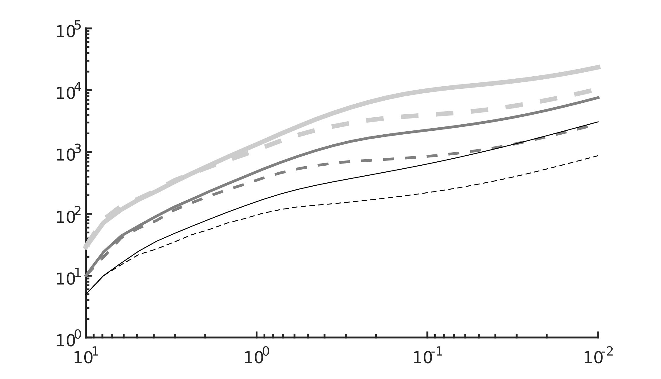
Figure 7: Cumulated number of iterations with respect to $\lambda_{n}$, for different parameters. Dashed lines: warm 3D with $N_{wr}=30$ (from thin dark gray to thick light gray: $\varepsilon_{wr}=\{10^{-4},10^{-5},10^{-6}\}$). Solid lines: classic Tikhonov (from thin dark gray to thick light gray: $\varepsilon_{wr}=\{10^{-4},10^{-5},10^{-6}\}$).

8.2 Parameter selection

In this section, we discuss the problem of the regularization parameter selection. We note again that iterative regularization provide a different way to explore different regularization level, and not a way to choose the right level. For the (3-D) method, the number of iterations $n$ is the regularization parameter, as shown in Proposition 7.1. The problem of choosing the right regularization level– i.e. the right regularization parameter– is of paramount important and still one of the biggest challenges in inverse problems. For illustration purposes, in previous numerical experiments, we used the original image $\bar{x}$ to find the iterate $\bar{n}$ for which the ground truth gap $GTG(x_{n})$ was minimized. This parameter’s choice is clearly unrealistic in practical situations, where we only have access to a noisy data $\hat{y}$. Many automatic parameters choice are known, e.g. Morozov’s discrepancy principle [50], or SURE [70]). Next, we comment on how they can be adapted to (3-D) and in particular, consider the SURE parameter selection method, that we briefly present below.

Remember from (4.1) that our algorithm can be written as $x_{n+1}:=\text{Algorithm}(x_{n};\lambda_{n};\hat{y})$. By recurrence, we can then express each iterate $x_{n}$ as a function of the starting point and the data

$$x_{n}=\text{Algorithm}(..\ \text{Algorithm}(x_{0};\lambda_{0};\hat{y});..\ ;\lambda_{n};\hat{y}),$$

or, more compactly, $x_{n}=\mathcal{A}_{n}(x_{0};\hat{y})$. The SURE is an unbiased estimator for the Mean Squared Error,

$$MSE(x)=(1/d)\|A(x_{n}-\bar{x})\|^{2},$$

provided we have access to the noisy data $\hat{y}$ and the variance of the noise $\sigma^{2}$. This estimator is defined by:

$$SURE(x_{n}):=\frac{1}{d}\|Ax_{n}-\hat{y}\|^{2}+\frac{2\sigma^{2}}{d}\langle AD_{n},\xi\rangle,$$

where $\xi\sim\mathcal{N}(0,Id_{\mathbb{R}^{d}})$ and $D_{n}=\partial_{\hat{y}}\mathcal{A}_{n}(x_{0};\cdot)[\xi]$ is the weak directional derivative of $\mathcal{A}_{n}(x_{0};\cdot)$ at $\hat{y}$ in the direction $\xi$. For more details on this method, and how to compute it in practice, the reader might consult [45, Section 4]).

The SURE estimator is depicted in Figure 8, in the setting of Example 8.1. One can see, and this behavior was observed in all experiments, that the curve of $SURE(x_{n})$ oscillates and is not convex. This can be problematic when looking for a global minimum: the oscillations, together with the fact that the global minimum of $SURE$ often presents a sharp shape, do not allow to find a robust minimizer. To circumvent these artifacts, we applied the following heuristic, which proved to be efficient in our experiments: smoothing the curve of $SURE(x_{n})$, and defining the early stopping iterate $\hat{n}$ as the one minimizing the slope of this smoothed version of $SURE(x_{n})$.

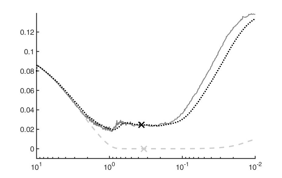
Figure 8: Plot of various estimators with respect to $\lambda_{n}$. Light gray dashed line: true MSE. Light gray cross: minimum of the true MSE. Gray plain line: SURE. Black dotted line: smoothed SURE. Black cross: minimum slope of the smoothed SURE. For display purposes, SURE and its smoothed version are here corrected by an additive constant.

Note that the statistical properties of the SURE estimator rely on the assumption that the noise is Gaussian [70, 45]. Nevertheless, as we will see below, it also provides surprisingly good results for the impulse noise, while being less efficient for the Poisson noise, or the mixed Gaussian-impulse noise.

8.3 Experiments for various noises and models

In this section, we run and compare vanilla 3D and warm 3D on a data-set, considering different noises and models for recovering the images. This data-set, which is available online, is made of 23 images, whose size range from $500\times 375$ to $515\times 512$ pixels. For each experiment, the range of parameters $(\lambda_{max},\lambda_{min})$ will be chosen accordingly to the nature of the noise and its variance. To fairly compare vanilla 3D and warm 3D, we will choose for each example the parameters $(N_{v},N_{wr},\varepsilon_{wr})$ in such a way that the number of iterations for both methods is of the same order ($\sim 10^{3}$). For each experiment, the early stopping will be defined according to two different rules: keeping the notations of Section 8.2, $\bar{n}$ will denote the iterate minimizing the ideal ground truth gap $GTG(x_{n})$, while $\hat{n}$ will be the iterate defined by means of the SURE estimator.

Example 8.2

Each image of the data-set is blurred and corrupted by a salt and pepper noise of intensity $35\%$, and is reconstructed by using an $L^{1}$ data-fit function $D(u,y)=\|u-y\|_{1}$, and a regularizer enforcing sparsity in a wavelet dictionary:

$$(\forall x\in X)\quad R(x)=\|Wx\|_{1}+\frac{1}{2}\|x\|^{2},$$

where here $W$ is a Daubechies wavelet transform. We run the (3-D) algorithm for $(\lambda_{max},\lambda_{min})=(10,10^{-1})$, and take $N_{v}=1000$ and $N_{wr}=20$, $\varepsilon_{wr}=10^{-5}$ for vanilla 3D and warm 3D, respectively. The results are summarized in Table 1 and Figure 9.

	vanilla 3D	warm 3D
Iterations	$1000$	$886\pm 160$
$GTG(x_{\bar{n}})$	$1{,}14.10^{-4}\pm 4{,}5.10^{-5}$	$1{,}11.10^{-4}\pm 4{,}3.10^{-5}$
$GTG(x_{\hat{n}})$	$1{,}37.10^{-4}\pm 5{,}8.10^{-5}$	$1{,}40.10^{-4}\pm 6{,}0.10^{-5}$

Table 1: Results of the experiments for Example 8.2.

$$\begin{array}[]{ccccc}\includegraphics[width=82.38885pt]{camera_noise.png}&\includegraphics[width=82.38885pt]{comete_noise.png}&\includegraphics[width=82.38885pt]{indian_noise.png}&\includegraphics[width=82.38885pt]{mountain_noise.png}&\includegraphics[width=82.38885pt]{raisins_noise.png}\\ \includegraphics[width=82.38885pt]{camera_vanilla_iterates.png}&\includegraphics[width=82.38885pt]{comete_vanilla_iterates.png}&\includegraphics[width=82.38885pt]{indian_vanilla_iterates.png}&\includegraphics[width=82.38885pt]{mountain_vanilla_iterates.png}&\includegraphics[width=82.38885pt]{raisins_vanilla_iterates.png}\\ \includegraphics[width=82.38885pt]{camera_vanilla_sugar.png}&\includegraphics[width=82.38885pt]{comete_vanilla_sugar.png}&\includegraphics[width=82.38885pt]{indian_vanilla_sugar.png}&\includegraphics[width=82.38885pt]{mountain_vanilla_sugar.png}&\includegraphics[width=82.38885pt]{raisins_vanilla_sugar.png}\\ \includegraphics[width=82.38885pt]{camera_warm_iterates.png}&\includegraphics[width=82.38885pt]{comete_warm_iterates.png}&\includegraphics[width=82.38885pt]{indian_warm_iterates.png}&\includegraphics[width=82.38885pt]{mountain_warm_iterates.png}&\includegraphics[width=82.38885pt]{raisins_warm_iterates.png}\\ \includegraphics[width=82.38885pt]{camera_warm_sugar.png}&\includegraphics[width=82.38885pt]{comete_warm_sugar.png}&\includegraphics[width=82.38885pt]{indian_warm_sugar.png}&\includegraphics[width=82.38885pt]{mountain_warm_sugar.png}&\includegraphics[width=82.38885pt]{raisins_warm_sugar.png}\end{array}$$

Figure 9: Samples from Example 8.2. From top to bottom: noisy image, reconstruction with vanilla 3D having access to the GTG (i.e. $x_{\bar{n}}$), reconstruction with vanilla 3D using SURE (i.e. $x_{\hat{n}}$), and reconstruction with warm 3D ($x_{\bar{n}}$ then $x_{\hat{n}}$).

Example 8.3

Each image of the data-set is blurred and corrupted by a salt and pepper noise of intensity $35\%$, and is reconstructed by using an $L^{1}$ data-fit function $D(u,y)=\|u-y\|_{1}$, and a regularizer based on the total variation:

$$(\forall x\in X)\quad R(x)=\frac{1}{10}\|x\|_{TV}+\frac{1}{2}\|x\|^{2}.$$

We run the (3-D) algorithm by taking $(\lambda_{max},\lambda_{min})=(10,10^{-1})$, with $N_{v}=1000$ and $N_{wr}=20$, $\varepsilon_{wr}=10^{-5}$ for vanilla 3D and warm 3D, respectively. The results are summarized in Table 2 and Figure 10.

	vanilla 3D	warm 3D
Iterations	$1000$	$618\pm 106$
$GTG(x_{\bar{n}})$	$1{,}02.10^{-4}\pm 4{,}3.10^{-5}$	$1{,}04.10^{-4}\pm 4{,}0.10^{-5}$
$GTG(x_{\hat{n}})$	$1{,}05.10^{-4}\pm 4{,}4.10^{-5}$	$1{,}13.10^{-4}\pm 4{,}1.10^{-5}$

Table 2: Results of the experiments for Example 8.3.

$$\begin{array}[]{ccccc}\includegraphics[width=82.38885pt]{boats_noise.png}&\includegraphics[width=82.38885pt]{butterfly_noise.png}&\includegraphics[width=82.38885pt]{girl_noise.png}&\includegraphics[width=82.38885pt]{barb_noise.png}&\includegraphics[width=82.38885pt]{louvre_noise.png}\\ \includegraphics[width=82.38885pt]{boats_vanilla_iterates.png}&\includegraphics[width=82.38885pt]{butterfly_vanilla_iterates.png}&\includegraphics[width=82.38885pt]{girl_vanilla_iterates.png}&\includegraphics[width=82.38885pt]{barb_vanilla_iterates.png}&\includegraphics[width=82.38885pt]{louvre_vanilla_iterates.png}\\ \includegraphics[width=82.38885pt]{boats_vanilla_sugar.png}&\includegraphics[width=82.38885pt]{butterfly_vanilla_sugar.png}&\includegraphics[width=82.38885pt]{girl_vanilla_sugar.png}&\includegraphics[width=82.38885pt]{barb_vanilla_sugar.png}&\includegraphics[width=82.38885pt]{louvre_vanilla_sugar.png}\\ \includegraphics[width=82.38885pt]{boats_warm_iterates.png}&\includegraphics[width=82.38885pt]{butterfly_warm_iterates.png}&\includegraphics[width=82.38885pt]{girl_warm_iterates.png}&\includegraphics[width=82.38885pt]{barb_warm_iterates.png}&\includegraphics[width=82.38885pt]{louvre_warm_iterates.png}\\ \includegraphics[width=82.38885pt]{boats_warm_sugar.png}&\includegraphics[width=82.38885pt]{butterfly_warm_sugar.png}&\includegraphics[width=82.38885pt]{girl_warm_sugar.png}&\includegraphics[width=82.38885pt]{barb_warm_sugar.png}&\includegraphics[width=82.38885pt]{louvre_warm_sugar.png}\end{array}$$

Figure 10: Samples from Example 8.3. From top to bottom: noisy image, reconstruction with vanilla 3D having access to the GTG (i.e. $x_{\bar{n}}$), reconstruction with vanilla 3D using SURE (i.e. $x_{\hat{n}}$), and reconstruction with warm 3D ($x_{\bar{n}}$ then $x_{\hat{n}}$).

Example 8.4

Each image of the data-set is blurred and corrupted by a Gaussian noise of variance $10^{-2}$, and is reconstructed by using an $L^{2}$ data-fit function $D(u,y)=(1/2)\|u-y\|^{2}$, and a regularizer based on the total variation:

$$(\forall x\in X)\quad R(x)=\|x\|_{TV}+\frac{1}{2}\|x\|^{2}.$$

We run the (3-D) algorithm by taking $(\lambda_{max},\lambda_{min})=(1,10^{-2})$, with $N_{v}=1000$ and $N_{wr}=20$, $\varepsilon_{wr}=10^{-4}$ for vanilla 3D and warm 3D, respectively. The results are summarized in Table 3 and Figure 11.

	vanilla 3D	warm 3D
Iterations	$1000$	$1096\pm 50$
$GTG(x_{\bar{n}})$	$1{,}41.10^{-4}\pm 4{,}4.10^{-5}$	$1{,}42.10^{-4}\pm 4{,}4.10^{-5}$
$GTG(x_{\hat{n}})$	$1{,}48.10^{-4}\pm 4{,}1.10^{-5}$	$1{,}56.10^{-4}\pm 3{,}9.10^{-5}$

Table 3: Results of the experiments for Example 8.4.

$$\begin{array}[]{ccccc}\includegraphics[width=82.38885pt]{flowers_noise.png}&\includegraphics[width=82.38885pt]{lena_noise.png}&\includegraphics[width=82.38885pt]{monkey_noise.png}&\includegraphics[width=82.38885pt]{pepper_noise.png}&\includegraphics[width=82.38885pt]{village_noise.png}\\ \includegraphics[width=82.38885pt]{flowers_vanilla_iterates.png}&\includegraphics[width=82.38885pt]{lena_vanilla_iterates.png}&\includegraphics[width=82.38885pt]{monkey_vanilla_iterates.png}&\includegraphics[width=82.38885pt]{pepper_vanilla_iterates.png}&\includegraphics[width=82.38885pt]{village_vanilla_iterates.png}\\ \includegraphics[width=82.38885pt]{flowers_vanilla_sugar.png}&\includegraphics[width=82.38885pt]{lena_vanilla_sugar.png}&\includegraphics[width=82.38885pt]{monkey_vanilla_sugar.png}&\includegraphics[width=82.38885pt]{pepper_vanilla_sugar.png}&\includegraphics[width=82.38885pt]{village_vanilla_sugar.png}\\ \includegraphics[width=82.38885pt]{flowers_warm_iterates.png}&\includegraphics[width=82.38885pt]{lena_warm_iterates.png}&\includegraphics[width=82.38885pt]{monkey_warm_iterates.png}&\includegraphics[width=82.38885pt]{pepper_warm_iterates.png}&\includegraphics[width=82.38885pt]{village_warm_iterates.png}\\ \includegraphics[width=82.38885pt]{flowers_warm_sugar.png}&\includegraphics[width=82.38885pt]{lena_warm_sugar.png}&\includegraphics[width=82.38885pt]{monkey_warm_sugar.png}&\includegraphics[width=82.38885pt]{pepper_warm_sugar.png}&\includegraphics[width=82.38885pt]{village_warm_sugar.png}\end{array}$$

Figure 11: Samples from Example 8.4. From top to bottom: noisy image, reconstruction with vanilla 3D having access to the GTG (i.e. $x_{\bar{n}}$), reconstruction with vanilla 3D using SURE (i.e. $x_{\hat{n}}$), and reconstruction with warm 3D ($x_{\bar{n}}$ then $x_{\hat{n}}$).

Example 8.5

Each image of the data-set is blurred and corrupted by a combination of a Gaussian noise of variance $5.10^{-3}$ and a salt and pepper noise of intensity $5\%$, and is reconstructed using an Huber data-fit function $D(u,y)=H_{\sigma}(x-y)$ with $\sigma=0.1$, and a regularizer based on the total variation:

$$(\forall x\in X)\quad R(x)=\|x\|_{TV}+\frac{1}{2}\|x\|^{2}.$$

We run the (3-D) algorithm by taking $(\lambda_{max},\lambda_{min})=(10^{-1},10^{-3})$, with $N_{v}=1000$ and $N_{wr}=20$, $\varepsilon_{wr}=10^{-4}$ for vanilla 3D and warm 3D, respectively. The results are summarized in Table 4 and Figure 12.

	vanilla 3D	warm 3D
Iterations	$1000$	$3760\pm 131$
$GTG(x_{\bar{n}})$	$1{,}56.10^{-4}\pm 4{,}3.10^{-5}$	$1{,}58.10^{-4}\pm 4{,}3.10^{-5}$
$GTG(x_{\hat{n}})$	$2{,}16.10^{-4}\pm 6{,}8.10^{-5}$	$1{,}99.10^{-4}\pm 8{,}2.10^{-5}$

Table 4: Results of the experiments for Example 8.5.

$$\begin{array}[]{ccccc}\includegraphics[width=82.38885pt]{boat_noise.png}&\includegraphics[width=82.38885pt]{bridge_noise.png}&\includegraphics[width=82.38885pt]{flower_noise.png}&\includegraphics[width=82.38885pt]{indian_noise_GSP.png}&\includegraphics[width=82.38885pt]{woman_noise.png}\\ \includegraphics[width=82.38885pt]{boat_vanilla_iterates.png}&\includegraphics[width=82.38885pt]{bridge_vanilla_iterates.png}&\includegraphics[width=82.38885pt]{flower_vanilla_iterates.png}&\includegraphics[width=82.38885pt]{indian_vanilla_iterates_GSP.png}&\includegraphics[width=82.38885pt]{woman_vanilla_iterates.png}\\ \includegraphics[width=82.38885pt]{boat_vanilla_sugar.png}&\includegraphics[width=82.38885pt]{bridge_vanilla_sugar.png}&\includegraphics[width=82.38885pt]{flower_vanilla_sugar.png}&\includegraphics[width=82.38885pt]{indian_vanilla_sugar_GSP.png}&\includegraphics[width=82.38885pt]{woman_vanilla_sugar.png}\\ \includegraphics[width=82.38885pt]{boat_warm_iterates.png}&\includegraphics[width=82.38885pt]{bridge_warm_iterates.png}&\includegraphics[width=82.38885pt]{flower_warm_iterates.png}&\includegraphics[width=82.38885pt]{indian_warm_iterates_GSP.png}&\includegraphics[width=82.38885pt]{woman_warm_iterates.png}\\ \includegraphics[width=82.38885pt]{boat_warm_sugar.png}&\includegraphics[width=82.38885pt]{bridge_warm_sugar.png}&\includegraphics[width=82.38885pt]{flower_warm_sugar.png}&\includegraphics[width=82.38885pt]{indian_warm_sugar_GSP.png}&\includegraphics[width=82.38885pt]{woman_warm_sugar.png}\end{array}$$

Figure 12: Samples from example 8.5. From top to bottom: noisy image, reconstruction with vanilla 3D having access to the GTG (i.e. $x_{\bar{n}}$), reconstruction with vanilla 3D using SURE (i.e. $x_{\hat{n}}$), and reconstruction with warm 3D ($x_{\bar{n}}$ then $x_{\hat{n}}$).

Example 8.6

Each image of the data-set is blurred and corrupted by a Poisson noise, and is reconstructed by using a Kullback-Leibler data-fit function $D(u,y)=\mathrm{KL}(y;u+b)$, where $b$ models a background noise of small intensity, and a regularizer based on the total variation:

$$(\forall x\in X)\quad R(x)=\frac{1}{10}\|x\|_{TV}+\frac{1}{2}\|x\|^{2}.$$

We run the (3-D) algorithm by taking $(\lambda_{max},\lambda_{min})=(10^{-1},10^{-3})$, with $N_{v}=1000$ and $N_{wr}=20$, $\varepsilon_{wr}=10^{-4}$ for vanilla 3D and warm 3D, respectively. The results are summarized in Table 5 and Figure 13.

	vanilla 3D	warm 3D
Iterations	$1000$	$3674\pm 329$
$GTG(x_{\bar{n}})$	$1{,}24.10^{-4}\pm 4{,}2.10^{-5}$	$1{,}26.10^{-4}\pm 4{,}2.10^{-5}$
$GTG(x_{\hat{n}})$	$3{,}51.10^{-4}\pm 3{,}9.10^{-5}$	$6{,}80.10^{-4}\pm 1{,}93.10^{-4}$

Table 5: Results of the experiments for Example 8.6.

$$\begin{array}[]{ccccc}\includegraphics[width=82.38885pt]{base_noise.png}&\includegraphics[width=82.38885pt]{brain_noise.png}&\includegraphics[width=82.38885pt]{parrot_noise.png}&\includegraphics[width=82.38885pt]{pepper_noise_P.png}&\includegraphics[width=82.38885pt]{pistil_noise.png}\\ \includegraphics[width=82.38885pt]{base_vanilla_iterates.png}&\includegraphics[width=82.38885pt]{brain_vanilla_iterates.png}&\includegraphics[width=82.38885pt]{parrot_vanilla_iterates.png}&\includegraphics[width=82.38885pt]{pepper_vanilla_iterates_P.png}&\includegraphics[width=82.38885pt]{pistil_vanilla_iterates.png}\\ \includegraphics[width=82.38885pt]{base_vanilla_sugar.png}&\includegraphics[width=82.38885pt]{brain_vanilla_sugar.png}&\includegraphics[width=82.38885pt]{parrot_vanilla_sugar.png}&\includegraphics[width=82.38885pt]{pepper_vanilla_sugar_P.png}&\includegraphics[width=82.38885pt]{pistil_vanilla_sugar.png}\\ \includegraphics[width=82.38885pt]{base_warm_iterates.png}&\includegraphics[width=82.38885pt]{brain_warm_iterates.png}&\includegraphics[width=82.38885pt]{parrot_warm_iterates.png}&\includegraphics[width=82.38885pt]{pepper_warm_iterates_P.png}&\includegraphics[width=82.38885pt]{pistil_warm_iterates.png}\\ \includegraphics[width=82.38885pt]{base_warm_sugar.png}&\includegraphics[width=82.38885pt]{brain_warm_sugar.png}&\includegraphics[width=82.38885pt]{parrot_warm_sugar.png}&\includegraphics[width=82.38885pt]{pepper_warm_sugar_P.png}&\includegraphics[width=82.38885pt]{pistil_warm_sugar.png}\end{array}$$

Figure 13: Samples from Example 8.6. From top to bottom: noisy image, reconstruction with vanilla 3D having access to the GTG (i.e. $x_{\bar{n}}$), reconstruction with vanilla 3D using SURE (i.e. $x_{\hat{n}}$), and reconstruction with warm 3D ($x_{\bar{n}}$ then $x_{\hat{n}}$).

As can be seen in the above experiments, the results achieved by the vanilla 3D method and the state-of-the-art warm 3D method are qualitatively comparable. Looking at the ideal early stopping rule ${\bar{n}}$, we see that they both perform very well in presence of impulse noise and Poisson noise (Examples 8.2, 8.3 and 8.6), and quite well in presence of Gaussian noise and mixed Gaussian-impulse noise (Examples 8.4 and 8.5). Concerning the early stop $\hat{n}$ defined with the SURE estimator, it provided good reconstructions for Gaussian and impulse noise, but less satisfactory ones for the Poisson noise, and mixed Gaussian-impulse noise. In the latter cases, the blur is removed but the image is contaminated by the noise, due to a late stopping. This suggests that an appropriate stopping rule should be investigated for these specific noises.

We emphasize that the practical performance of warm 3D, its computational time, and the shape of the sequence $(\lambda_{n})_{n\in\mathbb{N}}$, is crucially affected by the choice of $\varepsilon_{wr}$. For instance, in Examples 8.2 and 8.3, $\varepsilon_{wr}=10^{-5}$ and the number of iterations is around $700$, while in Examples 8.5 and 8.6, $\varepsilon_{wr}$ is taken as $10^{-4}$ but the number of iterations is larger (around $3700$). We see then in the vanilla 3D method an advantage, which is its direct control on the complexity of the method, thanks to the a priori choice of $N_{v}$. This can be of interest in practice, if one has a fixed computational budget.

9 Conclusion

In this paper we propose and analyze the (3-D) algorithm, a new iterative regularization method for solving ill-posed inverse problems, and show very good performances in practical imaging problems. To the best of our knowledge this is the first iterative regularization scheme that allows to consider general data fit terms and general regularizers, hence offering an alternative to standard Tikhonov approaches. The method is based on the forward-backward algorithm applied to a dual problem in a diagonal fashion. The proposed framework encompasses in particular the warm restart technique often used for classical Tikhonov regularization.

Our study opens many venues for future research. For example, our stability result appears to be suboptimal, since better result are known in special cases. It would then be interesting to see if it can be improved. Moreover, in our analysis we assume a solution of the linear inverse problem to exists, and it would be interesting to relax this assumption. Finally, considering convex, rather than strongly convex, regularization would be of interesting.

10 Appendix

10.1 Proofs for Section 2

Proof. [of Lemma 2.1] By [14, Theorem 18.15] $f^{*}$ is differentiable on $H_{1}$, and by [14, Proposition 16.23], $\nabla f^{*}=(\partial f)^{-1}$. Let $x\in H_{1}$ and $u\in\partial f(x)$. Since $W$ is surjective and ${\sigma}\|\cdot-x^{\prime}\|^{2}/2$ has full domain, it follows from [14, Proposition 16.42] that

$$u\in W^{*}\partial J(Wx)+\sigma(x-x^{\prime}).$$

Orthogonality of $W$ implies $\sigma^{-1}Wu\in\sigma^{-1}\partial J(Wx)+W(x-x^{\prime})$, and hence

$$(\sigma^{-1}Wu+Wx^{\prime})\in(\sigma^{-1}\partial J+I)(Wx).$$

The definition of proximity operator and the orthogonality of $W$ yield

$$x=W^{*}\mbox{\rm prox}_{\sigma^{-1}J}(\sigma^{-1}Wu+Wx^{\prime})=\nabla f^{*}(u).$$

     

10.2 Proofs for Section 4

We start computing the conditioning modulus of various data-fit function terms and we establish the properties we use.

Lemma 10.1

Let $d\in\mathbb{N}^{*}$, let $Y=\mathbb{R}^{d}$, and suppose that (AD) is satisfied. Then, the following hold.

1. Suppose that $D_{y}=\|\cdot-y\|^{p}/p$ with $p\in\left]1,2\right]$. Then its conditioning modulus satisfies

   $$(\forall t\in\mathbb{R})\ \ m(t)=|t|^{p}/p,\ \text{ and }\ m^{*}(t)=|t|^{q}/q,$$

   where $q$ is the conjugate exponent of $p$.

2. Suppose $D_{y}=\|\cdot-y\|_{1}$. Then its conditioning modulus satisfies

   $$(\forall t\in\mathbb{R})\ \ m(t)=|t|,\ \text{ and }\ m^{*}(t)=\delta_{[-1,1]}.$$

3. Suppose $D_{y}=\alpha_{1}\|\cdot-y\|_{1}\#(\alpha_{2}/2)\|\cdot-y\|^{2}$ for some $(\alpha_{1},\alpha_{2})\in\mathbb{R}_{++}^{2}$. Then its conditioning modulus satisfies, for every $t\in\mathbb{R}$,

   $$m(t)=\alpha_{1}h_{\frac{\alpha_{2}}{\alpha_{1}}}(t)\quad h^{*}(t)=\alpha_{1}\delta_{[-\alpha_{1},\alpha_{1}]}(t)+\frac{1}{2\alpha_{2}}t^{2},$$

   where $h_{\frac{\alpha_{2}}{\alpha_{1}}}$ is the function defined in (3.2).

The proof of the above lemma is straightforward and it is omitted. The computation of the conditioning modulus of the Kullback-Leibler divergence is more involved, and is done in the next lemma.

Lemma 10.2

Let $y\in]0,+\infty[^{d}$, and $D_{y}=\mathrm{KL}(y;\cdot)$.

1. Let $c=d\|y\|_{\infty}$. A conditioning modulus for $D_{y}$ is

   $$(\forall t\in\mathbb{R})\ \ m(t):=|t|-c\ln\left(1+c^{-1}|t|\right).$$

2. $m^{*}(t)=\begin{cases}-c(|t|+\ln(1-|t|))&\text{ if }t\in]-1,1[,\\ +\infty&\text{ otherwise.}\end{cases}$

3. $m(t)=\frac{1}{2c}t^{2}+o(t^{2})$ and $m^{*}(t)=\frac{c}{2}t^{2}+o(t^{2})$ for $t\to 0$.

Proof. In this proof we use the notations of Example 3.3. We will consider, for all $\alpha>0$ and $t\in\mathbb{R}$,

$$m_{\alpha}(t):=\mathrm{kl}(\alpha,\alpha+|t|)=\alpha\ln\left(\frac{\alpha}{\alpha+|t|}\right)+|t|.$$

According to [13], $m_{\alpha}\in\Gamma_{0}(\mathbb{R})$. Moreover, $\operatorname{argmin}m_{\alpha}=\{0\}$, so $t\mapsto m_{\alpha}(t)$ is an increasing function on $[0,+\infty[$. For all $t\in\mathbb{R}$, $\alpha\mapsto m_{\alpha}(t)$ is decreasing, since

$$\forall\alpha>0,\ \frac{{\rm d}}{{\rm d}\alpha}m_{\alpha}(t)=\ln\left(\frac{\alpha}{\alpha+|t|}\right)-\frac{\alpha}{\alpha+|t|}+1\leq 0.$$

Let us start by showing a one dimensional analogue of (2.3):

$$\forall\alpha>0,\forall\beta\in\mathbb{R},\ m_{\alpha}(|\beta-\alpha|)\leq\mathrm{kl}(\alpha,\beta).$$ (10.1)

Note that when $\beta\leq 0$, (10.1) is trivially satisfied because $\mathrm{kl}(\alpha,\beta)=+\infty$. Moreover, if $\beta\geq\alpha$, we have by definition of $m_{\alpha}$ that $m_{\alpha}(|\beta-\alpha|)=\mathrm{kl}(\alpha,\beta)$. So without loss of generality, we can assume that $\beta\in]0,\alpha[$. In this case, $m_{\alpha}(|\beta-\alpha|)=\mathrm{KL}(\alpha,\alpha+(\alpha-\beta))$. Introduce now the function

$$\xi_{\alpha}:t\in[0,\alpha[\ \longmapsto\mathrm{kl}(\alpha,\alpha-t)-\mathrm{kl}(\alpha,\alpha+t).$$

It suffices to prove that $\xi_{\alpha}(t)\geq 0$ on $]0,\alpha[$ and then take $t=\alpha-\beta\in]0,\alpha[$ to obtain (10.1). To prove this, first observe that $\xi_{\alpha}(0)=0$, and then observe that $\xi_{\alpha}$ is increasing on $]0,\alpha[$ by computing its derivative:

$$\forall t\in]0,\alpha[,\ \frac{{\rm d}}{{\rm d}t}\xi_{\alpha}(t)=\frac{2t^{2}}{\alpha^{2}-t^{2}}\geq 0.$$

Now that (10.1) is proved, let us prove item 1. Start by considering $y=(y_{i})_{i\in\{1,...,d\}}$ and $x=(x_{i})_{i\in\{1,...,d\}}$ in $\mathbb{R}^{d}_{++}$, and let $y_{\infty}:=\max\{y_{i}\ |\ i\in\{1,...,d\}\}$. Thanks to (10.1), we can write

$$\mathrm{KL}(y,x)=\sum\limits_{i=1}^{d}\mathrm{kl}(y_{i},x_{i})\geq\sum\limits_{i=1}^{d}m_{y_{i}}(|x_{i}-y_{i}|).$$ (10.2)

By using the fact that $\alpha\mapsto m_{\alpha}(t)$ is decreasing, we can bound the above estimate from below with

$$\mathrm{KL}(y,x)\geq\sum\limits_{i=1}^{d}m_{y_{\infty}}(|x_{i}-y_{i}|).$$

Then, by using Jensen inequality applied to the convex function $m_{y_{\infty}}$, we deduce that

$$\frac{1}{d}\mathrm{KL}(y,x) \geq m_{y_{\infty}}\left(\sum\limits_{i=1}^{d}\frac{1}{d}|x_{i}-y_{i}|\right)=m_{y_{\infty}}\left(\frac{1}{d}\|x_{i}-y_{i}\|_{1}\right).$$

But an easy computation shows that $m_{\alpha}(t/d)=m_{d\alpha}(t)/d$, so that

$$\frac{1}{d}\mathrm{KL}(y,x)\geq\frac{1}{d}m_{dy_{\infty}}\left(\|x-y\|_{1}\right).$$

By observing the fact that $\|x-y\|_{1}\geq\|x-y\|$ and recalling that $m_{dy_{\infty}}$ is an increasing function, we finally obtain $\mathrm{KL}(y,x)\geq m_{dy_{\infty}}(\|x-y\|)$, which proves item 1.

We next prove 2, by computing the Fenchel conjugate of $m$. Since $m(t)=m_{c}(t)=cm_{1}(t/c)$, we derive $m^{*}(t)=cm_{1}^{*}(t)$. We then just have to compute

$$m^{*}_{1}(t)=\sup\limits_{s\in\mathbb{R}}\ \eta_{t}(s),\text{ with }\eta_{t}(s)=\ st-|s|+\ln(1+|s|),$$

for every $s\in\mathbb{R}$. If $t=0$, we see from $\eta_{0}\leq 0$ and $\eta_{0}(0)=0$ that $\eta_{0}$ is maximized at $0$, whence $m_{1}^{*}(0)=0$. If $t\in\left]0,1\right[$, we have

$$\frac{{\rm d}}{{\rm d}s}\eta_{t}(s)=t-1+\frac{1}{1+s}\ \text{ on }\mathbb{R}_{++},$$

which is zero at $s=\frac{t}{1-t}\in\mathbb{R}_{++}$. Since $\eta_{t}$ is concave, this means that it is maximized there, whence $m_{1}^{*}(t)=-t-\ln(1-t)$. If $t\in]-1,0[$, the same argument shows that $\eta_{t}$ is maximized at $s=\frac{t}{1+t}\in\left]-\infty,0\right[$, leading in this case to $m_{1}^{*}(t)=t-\ln(1+t)$. From all of this, we see that $m_{1}^{*}(t)=|t|-\ln(1-|t|)$ on $]-1,1[$. Moreover, $m_{1}^{*}(t)$ tends to $+\infty$ when $|t|\to 1$, so from the convexity of $m_{1}^{*}$ we deduce that $m_{1}^{*}(t)\equiv+\infty$ when $|t|\geq 1$.

Item 3 is a simple consequence of item 2 and the classic Taylor expansion

$$\ln(1+t)=t-\frac{1}{2}t^{2}+o(t^{2})\ \text{ when }t\to 0.$$

     

10.3 Proofs for Section 6

Lemma 10.3

Let $f,g\in\Gamma_{0}(\mathbb{R})$ and let $a\in]0,+\infty]$. Suppose that, $f\leq g$ in $\left]-a,a\right[$. If $\text{\rm argmin}\ g=\{0\}$, then there exists $\varepsilon\in\mathbb{R}_{++}$ such that

$$\forall t\in]-\varepsilon,\varepsilon[,\ f^{*}(t)\geq g^{*}(t).$$

Proof. First, note that $\partial g^{*}(0)=\text{\rm argmin}\ g=\{0\}$ implies that $0\in\mbox{\rm int}\mathop{\mathrm{missing}}{\rm dom}g^{*}$ (see [14, Prop. 11.12 & 14.16]). Let $\varepsilon_{1}>0$ be such that $]-\varepsilon_{1},\varepsilon_{1}[\subset\mbox{\rm int}\mathop{\mathrm{missing}}{\rm dom}g^{*}$. Then $\partial g^{*}$ is nonempty on $\left]-\varepsilon_{1},\varepsilon_{1}\right[$, and we can define a function $\eta\colon\left]-\varepsilon_{1},\varepsilon_{1}\right[\to\mathbb{R}$, such that $\eta(t)\in\partial g^{*}(t)$ for all $t\in]-\varepsilon_{1},\varepsilon_{1}[$. We derive from [14, Th. 17.31] and [14, Prop. 17.36] that $\eta$ is continuous at zero. Now we are ready to prove the desired inequality. By using the Fenchel-Young inequality successively on $g$ and $f$, we write for all $t\in]-\varepsilon_{1},\varepsilon_{1}[$:

$$g(\eta(t))+g^{*}(t)=t\eta(t)\leq f(\eta(t))+f^{*}(t).$$

From the continuity of $\eta$ at zero, we infer the existence of some $\varepsilon_{2}\in]0,\varepsilon_{1}[$ such that $|t|<\varepsilon_{2}\Rightarrow|\eta(t)|<a$. We deduce from our assumption that $f(\eta(t))\leq g(\eta(t))$ holds for any $t\in]-\varepsilon_{2},\varepsilon_{2}[$, and the conclusion follows.      

Proof. [of Lemma 6.6] Let us start by proving $\Rightarrow$. Assume that there exists some $u^{\dagger}\in\operatorname{argmin}d$. Define $\tilde{x}:=\nabla f^{*}(-A^{*}u^{\dagger})$, which is equivalent to say that $0\in A^{*}u^{\dagger}+\partial f(\tilde{x})$. Using Fermat’s rule on $d$ at $u^{\dagger}$, we obtain that $A\nabla f^{*}(-A^{*}u^{\dagger})\in\partial g^{*}(u^{\dagger})$, which is equivalent to $u^{\dagger}\in\partial g(A\tilde{x})$. So we have

$$0\in\partial f(\tilde{x})+A^{*}\partial g(A\tilde{x}),$$ (10.3)

where a classic result [65, Corollary 3.31] shows that it implies $0\in\partial(f+g\circ A)(\tilde{x})$. Because of the strong convexity of $R$, this is a sufficient condition for $\tilde{x}$ to be the unique solution of ($P$), $x^{\dagger}$. It follows from (10.3) that we have $0\in\partial f(x^{\dagger})+A^{*}\partial g^{*}(Ax^{\dagger})$.

Now we turn on proving $\Leftarrow$, and we assume that there exists some $v\in\partial g(Ax^{\dagger})$ such that $-A^{*}v\in\partial f(x^{\dagger})$. Equivalently, $\nabla f^{*}(-A^{*}v)=x^{\dagger}$ holds, and this implies that $A\nabla f^{*}(-A^{*}v)=Ax^{\dagger}$. Since $v\in\partial g(Ax^{\dagger})\Leftrightarrow Ax^{\dagger}\in\partial g^{*}(v)$, we deduce that $A\nabla f^{*}(-A^{*}v)\in\partial g(v)$, which is a sufficient condition for $v$ to be a minimizer of $d$.

Now we end the proof by proving (6.14). Let $u\in Y,x:=\nabla f^{*}(-A^{*}u)$, $z\in\partial g^{*}(u)$, and we also take $z^{\dagger}:=Ax^{\dagger}$. Let $u^{\dagger}\in\operatorname{argmin}d$, so that by using a similar argument as above, we can write $x^{\dagger}=\nabla f^{*}(-A^{*}u^{\dagger})$, and deduce that $z^{\dagger}\in\partial g^{*}(u^{\dagger})$. Define the Lagrangian

$$L(x^{\prime},z^{\prime},u^{\prime}):=f(x^{\prime})+g(z^{\prime})+\langle u^{\prime},Ax^{\prime}-z^{\prime}\rangle,$$

and compute

$$L(x^{\dagger},z^{\dagger},u)-L(x,z,u)=f(x^{\dagger})-f(x)-\langle-A^{*}u,x^{\dagger}-x\rangle+g(z^{\dagger})-g(z)-\langle u,z^{\dagger}-z\rangle.$$

By using the fact that $f$ is $\sigma$-strongly convex with $-A^{*}u\in\partial f(x)$ and that $g$ is convex with $u\in\partial g(z)$, we deduce that

$$L(x^{\dagger},z^{\dagger},u)-L(x,z,u)\geq\frac{\sigma}{2}\|x-x^{\dagger}\|^{2}.$$ (10.4)

On the one hand, using again $-A^{*}u\in\partial f(x)$, $u\in\partial g(z)$ together with the Fenchel-Young theorem gives us

$$L(x,z,u)=-g^{*}(u)-f^{*}(-A^{*}u)=-d(u).$$ (10.5)

On the other hand, using $z^{\dagger}=Ax^{\dagger}$, $-A^{*}u^{\dagger}\in\partial f(x^{\dagger})$ and $u^{\dagger}\in\partial g(z^{\dagger})$ together with the Fenchel-Young theorem leads to

$$L(x^{\dagger},z^{\dagger},u) = f(x^{\dagger})+g(Ax^{\dagger})$$

$$= -f^{*}(-A^{*}u^{\dagger})-g^{*}(u^{\dagger})$$

$$= -d(u^{\dagger})=-\inf d.$$

The result follows then from (10.4), (10.5) and (10.3).      

10.4 Proofs for Section 7

Here we prove the estimations claimed in Example 5.6.

Lemma 10.4

Let $H$ be a Hilbert space, $G\in\Gamma_{0}(H)$ with $\text{\em argmin }G=\{0\}$. Let $(y_{1},y_{2})\in H^{2}$, and $\phi_{i}:=G(\cdot-y_{i})$ for $i\in\{1,2\}$. Then

$$\sup\limits_{\alpha>0}\ \sup\limits_{u\in H}\ \|\mbox{\rm prox}_{\alpha\phi_{1}}(u)-\mbox{\rm prox}_{\alpha\phi_{2}}(u)\|=\|y_{1}-y_{2}\|.$$ (10.7)

Proof. Let $\alpha\in\mathbb{R}_{++}$, and let $u\in H$. By using [37, Table 1.i], we can write for $i\in\{1,2\}$ that

$$\mbox{\rm prox}_{\alpha\phi_{i}}(u)=y_{i}+\mbox{\rm prox}_{\alpha G}(u-y_{i}).$$

Then it follows that

$$\|\mbox{\rm prox}_{\alpha\phi_{1}}(u)-\mbox{\rm prox}_{\alpha\phi_{2}}(u)\|=\|(\operatorname{Id}-\mbox{\rm prox}_{\alpha G})(u-y_{1})-(\operatorname{Id}-\mbox{\rm prox}_{\alpha G})(u-y_{2})\|.$$

By using first the firm non expansiveness of the proximity operator [14, Prop. 12.27], one directly obtains

$$\sup\limits_{\alpha>0}\ \sup\limits_{u\in H}\ \|\mbox{\rm prox}_{\alpha\phi_{1}}(u)-\mbox{\rm prox}_{\alpha\phi_{2}}(u)\|\leq\|y_{1}-y_{2}\|.$$ (10.8)

To achieve the equality in the inequality above, observe that $\mbox{\rm prox}_{\alpha G}(u-y_{i})$ converges strongly to zero when $\alpha\to+\infty$, by using [25, Lem. 1] and $\operatorname{argmin}G=\{0\}$. This implies that

$$\forall u\in H,\ \|\mbox{\rm prox}_{\alpha\phi_{1}}(u)-\mbox{\rm prox}_{\alpha\phi_{2}}(u)\|\overset{\alpha\to+\infty}{\relbar\joinrel\longrightarrow}\|y_{1}-y_{2}\|.$$

     

Lemma 10.5

Let $y_{1},y_{2}\in\mathbb{R}^{d}_{++}$, and $\phi_{i}:=\mathrm{KL}(y_{i},\cdot)$ for $i\in\{1,2\}$. Let $\alpha\in\mathbb{R}_{++}$. Then

$$\sup\limits_{u\in\mathbb{R}^{d}}\ \|\mbox{\rm prox}_{\alpha\phi_{1}}(u)-\mbox{\rm prox}_{\alpha\phi_{2}}(u)\|=\sqrt{\alpha}\|\sqrt{y_{1}}-\sqrt{y_{2}}\|,$$

where $\sqrt{y_{i}}$ shall be understood component-wise.

Proof. Let $u=(u_{j})_{j\in\{1,...,d\}}\in\mathbb{R}^{d}$, and let us denote $y_{i}=(y_{ij})_{j\in\{1,...,d\}}$ for $i\in\{1,2\}$. The proximity operator of $\alpha\phi_{i}$ at $u$ is defined component-wise by (see [31, 48])

$$\left(\mbox{\rm prox}_{\alpha\phi_{i}}(u)\right)_{j}=\frac{1}{2}\left(u_{j}-\alpha+\sqrt{(u_{j}-\alpha)^{2}+4\alpha y_{ij}}\right).$$

Then,

$$\|\mbox{\rm prox}_{\alpha\phi_{1}}(u)-\mbox{\rm prox}_{\alpha\phi_{2}}(u)\|^{2}=\frac{1}{4}\sum\limits_{j=1}^{d}\left|\sqrt{(u_{j}-\alpha)^{2}+4\alpha y_{1j}}-\sqrt{(u_{j}-\alpha)^{2}+4\alpha y_{2j}}\right|^{2}.$$

Let $(a,b)\in[0,+\infty]^{2}$, and define

$$\xi:t\in]0,+\infty[\mapsto\left|\sqrt{t+a}-\sqrt{t+b}\right|^{2}.$$

Since $\xi$ is decreasing on $\mathbb{R}_{+}$, by considering $u_{j}=\alpha$ for all $j\in\{1,\ldots,d\}$,

$$\sup\limits_{u_{j}\in\mathbb{R}}\left|\sqrt{(u_{j}-\alpha)^{2}+4\alpha y_{1j}}-\sqrt{(u_{j}-\alpha)^{2}+4\alpha y_{2j}}\right|^{2}=\left|\sqrt{4\alpha y_{1j}}-\sqrt{4\alpha y_{2j}}\right|^{2}=4\alpha|\sqrt{y_{1j}}-\sqrt{y_{2j}}|^{2}.$$

We then conclude that

$$\sup\limits_{u\in\mathbb{R}^{d}}\ \|\mbox{\rm prox}_{\alpha\phi_{1}}(u)-\mbox{\rm prox}_{\alpha\phi_{2}}(u)\|^{2}=\sum\limits_{j=1}^{d}\alpha|\sqrt{y_{1j}}-\sqrt{y_{2j}}|^{2}=\alpha\|\sqrt{y_{1}}-\sqrt{y_{2}}\|^{2}.$$

References

- [1] P. Alart and B. Lemaire, Penalization in non-classical convex programming via variational convergence, Mathematical Programming, 51, pp. 307–331, 1991.
- [2] F. Alvarez and R. Cominetti, Primal and dual convergence of a proximal point exponential penalty method for linear programming, Mathematical Programming, 93, pp. 87–96, 2002.
- [3] H. Attouch, Viscosity Solutions of Minimization Problems, SIAM Journal on Optimization, 6, pp. 769–806, 1996.
- [4] H. Attouch, A. Cabot, and M.-O. Czarnecki, Asymptotic behavior of non-autonomous monotone and subgradient evolution equations, arXiv:1601.00767, 2016.
- [5] H. Attouch and R. Cominetti, A dynamical approach to convex minimization coupling approximation with the steepest descent method, Journal of Differential Equations, 128, pp. 519-540, 1996.
- [6] H. Attouch and M.-O. Czarnecki, Asymptotic behavior of coupled dynamical systems with multiscale aspects, Journal of Differential Equations, 248, pp. 1315-1344, 2010.
- [7] H. Attouch, M.-O. Czarnecki, and J. Peypouquet, Prox-Penalization and Splitting Methods for Constrained Variational Problems, SIAM Journal on Optimization, 21, pp. 149–173, 2011.
- [8] H. Attouch, M.-O. Czarnecki, and J. Peypouquet, Coupling Forward-Backward with Penalty Schemes and Parallel Splitting for Constrained Variational Inequalities, SIAM Journal on Optimization, 21, pp. 1251–1274, 2011.
- [9] A. Auslender, J.-P. Crouzeix, and P. Fedit, Penalty-proximal methods in convex programming, Journal of Optimization Theory and Applications, 55, pp. 1–21, 1987.
- [10] M. Bachmayr and M. Burger, Iterative total variation schemes for nonlinear inverse problems, Inverse Problems 25, 105004, 26 pp., 2009.
- [11] M. A. Bahraoui and B. Lemaire, Convergence of diagonally stationary sequences in convex optimization, Set-Valued Analysis, 2, pp. 49–61, 1994.
- [12] A. B. Bakushinsky and M. Yu. Kokurin, Iterative Methods for Approximate Solution of Inverse Problems, Springer, New York, 2004.
- [13] H.H. Bauschke and J. Borwein, Joint and Separate Convexity of the Bregman Distance, in Studies in Computational Mathematics, Inherently Parallel Algorithms in Feasibility and Optimization and their Applications, 8, pp. 23–36, 2001.
- [14] H.H. Bauschke and P. Combettes, Convex analysis and monotone operator theory, Springer, New York, 2011.
- [15] A. Beck and S. Sabach, A first order method for finding minimal norm-like solutions of convex optimization problems, Mathematical Programming, 147, pp. 25–46, 2014.
- [16] A. Beck and M. Teboulle, Mirror descent and nonlinear projected subgradient methods for convex optimization, Operations Research Letters, 31, pp. 167–175, 2003.
- [17] S. Becker, J. Bobin, and E. Candès, NESTA: A Fast and Accurate First-Order Method for Sparse Recovery, SIAM Journal on Imaging Sciences, 4, pp. 1–39, 2011.
- [18] M. Bertero and P. Boccacci, Introduction to Inverse Problems in Imaging, IOP Publishing, Bristol and Philadelphia, 1998.
- [19] J. Bolte, T. P. Nguyen, J. Peypouquet, and B. Suter, From error bounds to the complexity of first-order descent methods for convex functions, arXiv:1510.08234, 2015.
- [20] R. I. Bot and B. Hofmann, The impact of a curious type of smoothness conditions on convergence rates in l1-regularization, Eurasian Journal of Mathematical and Computer Applications, 1, pp. 29–40, 2013.
- [21] R. I. Bot and T. Hein, Iterative regularization with a general penalty term: theory and application to L1 and TV regularization, Inverse Problems, 28, pp. 1–19, 2012.
- [22] R. Boyer, Quelques algorithmes diagonaux en optimisation convexe, Ph.D., Université de Provence, 1974.
- [23] K. Bredies, K. Kunisch, and T. Pock, Total generalized variation, SIAM Journal on Imaging Sciences, 3, pp. 492–526, 2010.
- [24] L. Briceño-Arias and P. L. Combettes, A monotone + skew splitting model for composite monotone inclusions in duality, SIAM Journal on Optimization 21, pp. 1230–1250, 2011.
- [25] R. E. Bruck Jr., A strongly convergent iterative solution of for a maximal monotone operator in Hilbert space, Journal of Mathematical Analysis and Applications, 48, pp. 114–126, 1974.
- [26] M. Burger and S. Osher, A guide to the TV zoo. In Level Set and PDE Based Reconstruction Methods in Imaging, pp. 1–70. Springer, 2013.
- [27] M. Burger, E. Resmerita, and L. He, Error estimation for Bregman iterations and inverse scale space methods in image restoration, Computing. Archives for Scientific Computing, 81, pp. 109–135, 2007.
- [28] A. Cabot, The steepest descent dynamical system with control. Applications to constrained minimization, ESAIM: Control, Optimisation and Calculus of Variations, 10, pp. 243–258, 2004.
- [29] A. Cabot, Proximal Point Algorithm Controlled by a Slowly Vanishing Term: Applications to Hierarchical Minimization, SIAM Journal on Optimization, 15, pp. 555–572, 2005.
- [30] L. Calatroni, J.-C. De Los Reyes, and C.-B. Schönlieb, Infimal convolution of data discrepancies for mixed noise removal, arXiv:1611.00690, 2016.
- [31] C. Chaux, P. L. Combettes, J.-C. Pesquet, and V. Wajs, A variational formulation for frame-based inverse problems, Inverse Problems 23, pp. 1495–1518, 2007.
- [32] A. Chambolle and P. L. Lions, Image recovery via total variation minimization and related problems, Numerische Mathematik, 76, pp. 167–188, 1997.
- [33] A. Chambolle and T. Pock, A First-Order Primal-Dual Algorithm for Convex Problems with Applications to Imaging, Journal of Mathematical Imaging and Vision 40, pp. 120–145, 2011.
- [34] A. Chambolle and T. Pock, A remark on accelerated block coordinate descent for computing the proximity operators of a sum of convex functions, preprint hal-01099182v2, 2015.
- [35] P. L. Combettes, Quasi-Fejérian analysis of some optimization algorithms, in Inherently Parallel Algorithms in Feasibility and Optimization and Their Applications, (D. Butnariu, Y. Censor, and S. Reich, Eds.), New York: Elsevier, pp. 115–152, 2001.
- [36] P. L. Combettes, D. Dũng, and B. C. Vũ, Dualization of signal recovery problems, Set-Valued and Variational Analysis, 18, pp. 373–404, 2010.
- [37] P. L. Combettes and J.-C. Pesquet, Proximal splitting methods in signal processing, in Fixed-point algorithms for inverse problems in science and engineering, pp. 185–212, Springer, New York, 2011.
- [38] P. L. Combettes and J.-C. Pesquet, Primal-dual splitting algorithm for solving inclusions with mixtures of composite, Lipschitzian, and parallel-sum type monotone operators. Set-Valued Variational Analysis 20, pp. 307–330, 2012.
- [39] P. L. Combettes and V. Wajs, Signal recovery by proximal forward-backward splitting, Multiscale Modeling & Simulation, 4, pp. 1168–1200, 2005.
- [40] R. Cominetti and O. Alemany, Steepest descent evolution equations: asymptotic behavior of solutions and rate of convergence, Transactions of the American Mathematical Society, 351, pp. 4847–4860, 1999.
- [41] R. Cominetti, J. Peypouquet, and S. Sorin, Strong asymptotic convergence of evolution equations governed by maximal monotone operators with Tikhonov regularization, Journal of Differential Equations, 245, pp. 3753–3763, 2008.
- [42] R. Cominetti, Coupling the Proximal Point Algorithm with Approximation Methods, Journal of Optimization Theory and Applications, 95, pp. 581–600, 1997.
- [43] M.-O. Czarnecki, N. Noun, and J. Peypouquet, Splitting forward-backward penalty scheme for constrained variational problems, arXiv:1408.0974, 2014.
- [44] I. Daubechies, M. Defrise, and C. De Mol, An Iterative Thresholding Algorithm for Linear Inverse Problems with a Sparsity Constraint, Communications on Pure and Applied Mathematics, 57, pp. 1413–1457, 2004.
- [45] C.-A. Deledalle, S. Vaiter, J.-M. Fadili, and G. Peyré, Stein Unbiased GrAdient estimator of the Risk (SUGAR) for multiple parameter selection, SIAM Journal on Imaging Sciences, 7, pp. 2448–2487, 2014.
- [46] D. Donoho and I Johnstone, Ideal spatial adaptation via wavelet shrinkage, Biometrika, 81, pp.425–455, 1994.
- [47] A. Dontchev and T. Zolezzi, Well-posed optimization problems, Springer-Verlag, Berlin, 1993.
- [48] F.-X. Dupé, J. Fadili, andj.-L. Starck, Deconvolution under Poisson noise using exact data-fit function and synthesis or analysis sparsity priors, Statistical Methodology, 9, pp. 4–18, 2012.
- [49] H. Egger, On the Convergence of modified Landweber iteration for nonlinear inverse problems, Johann Radon Institute Computational Applied Mathematics, Technical Report SFB-2010-017, 2010.
- [50] H. Engl, M. Hanke, and A. Neubauer, Regularization of Inverse Problems, Kluwer, Dordrecht, 1996.
- [51] E. Hale, W. Yin, and Y. Zhang, Fixed-Point Continuation for -Minimization: Methodology and Convergence, SIAM Journal on Optimization, 19, pp.1107–1130, 2008.
- [52] M. Hintermüller and A. Langer, Subspace correction methods for a class of non-smooth and non-additive convex variational problems with mixed data-fidelity in image processing, SIAM Journal on Imaging Sciences, 6, pp. 2134–2173, 2013.
- [53] B. Kaltenbacher, A. Neubauer and O. Scherzer, Iterative Regularization Methods for Nonlinear Ill-Posed Problems, De Gruyter, Berlin, 2008.
- [54] A. A. Kaplan, On Convex Programming with Internal Regularization, Soviet Mathematics, Doklady Akademii Nauk, 19, pp. 795–799, 1975.
- [55] A. A. Kaplan, Iteration processes of convex programming with internal regularization, Siberian Mathematical Journal, 20, pp. 219–226, 1979.
- [56] A. Langer, Automated Parameter Selection for Total Variation Minimization in Image Restoration, arXiv 1509.07442v3, 2015.
- [57] T. Le, R. Chartran, and T. Asaki,A variational approach to reconstructing images corrupted by Poisson noise, Journal of Mathematical Imaging and Vision, 27, pp. 257–63, 2007.
- [58] B. Lemaire, Coupling optimization methods and variational convergence, in Trends in Mathematical Optimization, International Series of Numerical Mathematics, 84, pp. 163–179, 1988.
- [59] B. Lemaire, On the Convergence of Some Iterative Methods for Convex Minimization, in Recent Developments in Optimization, Lecture Notes in Economics and Mathematical Systems, 429, pp. 252–268, 1995.
- [60] B. Lemaire, Well-posedness, conditioning and regularization of minimization, inclusion and fixed-point problems, Pliska Studia Mathematica Bulgarica, 12, pp. 71–84, 1998.
- [61] S. Mallat, A Wavelet Tour of Signal Processing, 3rd edition. Elsevier/Academic Press, Amsterdam, 2009.
- [62] B. Martinet, Perturbation des m thodes d’optimisation. Applications, R.A.I.R.O. - Analyse num rique, 12, pp. 153–171, 1978.
- [63] M. Nikolova, Minimizers of cost-functions involving non- smooth data-fidelity terms. Application to the processing of outliers., SIAM Journal of Numerical Analysis 40, pp. 965–994, 2002.
- [64] J. Peypouquet, Coupling the Gradient Method with a General Exterior Penalization Scheme for Convex Minimization, Journal of Optimization Theory and Applications, 153, pp. 123–138, 2011.
- [65] J. Peypouquet, Convex optimization in normed spaces. Theory, methods and examples., Springer, New York, 2015.
- [66] R. Ramlau, TIGRA – an iterative algorithm for regularizing nonlinear ill-posed problems, Inverse Problems, 19, pp. 433–465, 2003.
- [67] S. Matet, L. Rosasco, S .Villa, and B. C. Vũ, Don’t relax: early stopping for convex regularization, manuscript 2016.
- [68] L. Rudin, S. Osher, and E. Fatemi, Nonlinear total variation based noise removal algorithms, Physica D: Nonlinear Phenomena, 60, pp.259–268, 1992.
- [69] O. Scherzer, A Modified Landweber Iteration for Solving Parameter Estimation Problems, Applied Mathematics and Optimization, 38, pp. 45–68, 1998.
- [70] C. Stein, Estimation of the mean of a multivariate normal distribution, Annals of Statistics, 9, pp. 1135–1151, 1981.
- [71] I. Steinwart and A. Christmann, Support Vector Machines, Springer, New York, 2008.
- [72] P. Tossings, The perturbed Tikhonov’s algorithm and some of its applications, ESAIM: Mathematical Modelling and Numerical Analysis, 28, pp. 189–221, 1994.
- [73] P. Tseng, Applications of a Splitting Algorithm to Decomposition in Convex Programming and Variational Inequalities, SIAM Journal on Control and Optimization, 29, pp. 119–138, 1991.
- [74] H. Uzawa, Iterative methods for concave programming, in Studies in Linear and Nonlinear Programming, Stanford University Press, Stanford, pp. 154–165, 1958.
- [75] M. M. Vainberg, Le problème de la minimisation des fonctionelles non linéaires, C.I.M.E. IV ciclo (1970).
- [76] I. Yamada, M. Yukawa and M. Yamagishi, Minimizing the Moreau Envelope of Nonsmooth Convex Functions over the Fixed Point Set of Certain Quasi-Nonexpansive Mappings, in Fixed-Point Algorithms for Inverse Problems in Science and Engineering, Springer New York, 2011.
- [77] T. Zolezzi, On equiwellset minimum problems, Applied Mathematics and Optimization, 4, pp. 209–223, 1978.
- [78] Z. Zou and T. Hastie, Regularization and variable selection via the elastic net, Journal of the Royal Statistical Society, Series B, 67, pp. 301–320, 2005.
- [79] C. Zalinescu, Convex Analysis in General Vector Spaces, World Scientific, Singapore, 2002.