Deep Reinforcement Learning
From Raw Pixels in Doom

Abstract

Using current reinforcement learning methods, it has recently become possible to learn to play unknown 3D games from raw pixels. In this work, we study the challenges that arise in such complex environments, and summarize current methods to approach these. We choose a task within the Doom game, that has not been approached yet. The goal for the agent is to fight enemies in a 3D world consisting of five rooms. We train the DQN and LSTM-A3C algorithms on this task. Results show that both algorithms learn sensible policies, but fail to achieve high scores given the amount of training. We provide insights into the learned behavior, which can serve as a valuable starting point for further research in the Doom domain.

Chapter 1 Introduction

Understanding human-like thinking and behavior is one of our biggest challenges. Scientists approach this problem from diverse disciplines, including psychology, philosophy, neuroscience, cognitive science, and computer science. The computer science community tends to model behavior farther away from the biological example. However, models are commonly evaluated on complex tasks, proving their effectivity.

Specifically, reinforcement learning (RL) and intelligent control, two communities within machine learning and, more generally, artificial intelligence, focus on finding strategies to behave in unknown environments. This general setting allows methods to be applied to financial trading, advertising, robotics, power plant optimization, aircraft design, and more [1, 30].

This thesis provides an overview of current state-of-the-art algorithms in RL and applies a selection of them to the Doom video game, a recent and challenging testbed in RL.

The structure of this work is as follows: We motivate and introduce the RL setting in Chapter 1, and explain the fundamentals of RL methods in Chapter 2. Next, we discuss challenges that arise in complex environments like Doom in Chapter 3, describe state-of-the-art algorithms in Chapter 4, and conduct experiments in Chapter 5. We close with a conclusion in Chapter 6.

1.1 The Reinforcement Learning Setting

The RL setting defines an environment and an agent that interacts with it. The environment can be any problem that we aim to solve. For example, it could be a racing track with a car on it, an advertising network, or the stock market. Each environment reveals information to the agent, such as a camera image from the perspective of the car, the profile of a user that we want to display ads to, or the current stock prices.

The agent uses this information to interact with the environment. In our examples, the agent might control the steering wheel and accelerator, choose ads to display, or buy and sell shares. Moreover, the agent receives a reward signal that depends on the outcome of its actions. The problem of RL is to learn and choose the best action sequences in an initially unknown environment. In the field of control theory, we also refer to this as a control problem because the agent tries to control the environment using the available actions.

1.2 Human-Like Artificial Intelligence

RL has been used to model the behavior of humans and artificial agents. Doing so assumes that humans try to optimize a reward signal. This signal can be arbitrarily complex and could be learned both during lifetime and through evolution over the course of generations. For example, he neurotransmitter dopamine is known to play a critical role in motivation and is related to such a reward system in the human brain.

Modeling human behavior as an RL problem a with complex reward function is not completely agreed on, however. While any behavior can be modeled as following a reward function, simpler underlying principles than this could exist. These principles might be more valuable to model human behavior and build intelligent agents.

Moreover, current RL algorithms can hardly be compared with human behavior. For example, a common approach in RL algorithms is called probability matching, where the agent tries to choose actions relative to their probabilities of reward. Humans tend to prefer the small chance of a high reward over the highest expected reward. For further details, please refer to Shteingart and Loewenstein [22].

1.3 Relation to Supervised and Unsupervised Learning

Supervised learning (SL) is the dominant framework in the field of machine learning. It is fueled by successes in domains like computer vision and natural language processing, and the recent break-through of deep neural networks. In SL, we learn from labeled examples that we assume are independent. The objective is either to classify unseen examples or to predict a scalar property of them.

In comparison to SL, RL is more general by defining sequential problems. While not always useful, we could model any SL problem as a one-step RL problem. Another connection between the two frameworks is that many RL algorithms use SL internally for function approximation (Sections 2.6.1 and 3.1).

Unsupervised learning (UL) is an orthogonal framework to RL, where examples are unlabeled. Thus, unsupervised learning algorithms make sense from data by compression, reconstruction, prediction, or other unsupervised objectives. Especially in complex RL environments, we can employ methods from unsupervised learning to extract good representations to base decisions on (Section 3.1).

1.4 Reinforcement Learning in Games

The RL literature uses different testbeds to evaluate and compare its algorithms. Traditional work often focuses on simple tasks, such as balancing a pole on a cart in 2D. However, we want to build agents that can cope with the additional difficulties that arise in complex environments (Chapter 3).

Video games provide a convenient way to evaluate algorithms in complex environments, because their interface is clearly defined and many games define a score that we forward to the agent as the reward signal. Board games are also commonly addressed using RL approaches but are not considered in this work, because their rules are known in advance.

Most notably, the Atari environment provided by ALE [3] consists of 57 low-resolution 2D games. The agent can learn by observing either screen pixels or the main memory used by game. 3D environments where the agent observes perspective pixel images include the driving simulator Torcs [35], several similar block-world games that we refer to as Minecraft domain, and the first-person shooter game Doom [9] (Section 5.1).

Chapter 2 Reinforcement Learning Background

The field of reinforcement learning provides a general framework that models the interaction of an agent with an unknown environment. Over multiple time steps, the agent receives observations of the environment, responds with actions, and receives rewards. The actions affect the internal environment state.

For example, at each time step, the agent receives a pixel view of the Doom environment and chooses one of the available keyboard keys to press. The environment then advances the game by one time step. If the agent killed an enemy, we reward it with a positive signal of $1$, and otherwise with $0$. Then, the environment sends the next frame to the agent so that it can choose its next action.

2.1 Agent and Environment

Formally, we define the environment as partially observable Markov decision process (POMDP), consisting of a state space $S$, an action space $A$, and an observation space $X$. Further, we define a transition function $T\colon S\times A\rightarrow\mathrm{Dist}(S)$ that we also refer to as the dynamics, an observation function $O\colon S\rightarrow\mathrm{Dist}(X)$, and a reward function $R\colon S\times A\rightarrow\mathrm{Dist}(\mathbb{R})$, where $\mathrm{Dist}(D)$ refers to the space of random variables over $D$. We denote $T_{ss^{\prime}}^{a}=\Pr(T(s,a)=s^{\prime})$. The initial state is $s_{0}\in S$ and we model terminal states implicitly by having a recurrent transition probability of $1$ and a reward of $0$.

We use $O(s)$ to model that the agent might not be able observe the entire state of the environment. When $S=X$ and $\forall s\in S\colon\Pr(O(s)=s)=1$, the environment is fully observable, reducing the POMDP into a Markov decision process (MDP).

The agent defines a policy $\pi\colon\mathcal{P}(X)\rightarrow\mathrm{Dist}(A)$ that describes how it chooses actions based on previous observations from the environment. By convention, we denote the variable of the current action given previous observations as $\pi(x_{t})=\pi((x_{0},\dots,x_{t}))$ and the probability of choosing a particular action as $\pi(a_{t}|x_{t})=\Pr(\pi(x_{t})=a_{t})$. Initially, the agents provides an action $a_{0}$ based on the observation $x_{0}$ observed from $O(s_{0})$.

At each discrete time step $t\in\mathbb{N^{+}}$, the environment observes a state $s_{t}$ from $S(s_{t-1},a_{t-1})$. The agent then observes a reward $r_{t}$ from $R(s_{t-1},a_{t-1})$ and an observation $x_{t}$ from $O(s_{t})$. The environment then observes $a_{t}$ from the agent’s policy $\pi(x_{t})$.

We name a trajectory of all observations starting from $t=0$ an episode, and the tuples $(x_{t-1},a_{t-1},r_{t},x_{t})$ that the agent observes, transitions. Further, we write $E_{\pi}\left[\cdot\right]$ as the expectation over the episodes observed under a given policy $\pi$.

The return $R_{t}$ is a random variable describing the discounted rewards after $t$ with discount factor $\gamma\in\left[0,1\right)$. Without subscript, we assume $t=0$. Note that, although possibly confusing, we stick to the common notation of using the letter $R$ to denote both the reward function and the return from $t=0$.

$$R_{t}=\sum_{i=1}^{\infty}{\gamma^{i}R(s_{t+i},a_{t+i})}.$$

Note that the return is finite as long as the rewards have finite bounds. When all episodes of the MDP are finite, we can also allow $\gamma=1$, because the terminal states only add rewards of $0$ to the return.

The agent’s objective is to maximize the expected return $E_{\pi}\left[R\right]$ under its policy. The solution to this depends on the choice of $\gamma$: Values close to $1$ encourage long-sighted actions while values close to $0$ encourage short-sighted actions.

2.2 Value-Based Methods

RL methods can roughly be separated into value-based and policy-based (Section 2.7) ones. RL theory often assumes fully-observable environments, so for now, we assume that the agent found a way to reconstruct $s_{t}$ from the observations $x_{0},...x_{t}$. Of course, depending on $O$, this might not be completely possible. We discuss the challenge of partial observability later in Section 3.2.

An essential concept of value-based methods is the value function $V^{\pi}(s_{t})=\rm I\kern-3.00003pt\mathbb{E}_{\pi}\left[R_{t}\right]$. We use $V^{*}$ to denote the value function under an optimal policy. The value function has an interesting property, known as Bellman equation:

$$V^{\pi}(s)=\rm I\kern-3.00003pt\mathbb{E}_{\pi}\left[R(s,a)+\gamma\sum_{s^{\prime}\in S}{T_{ss^{\prime}}^{a}V^{\pi}(s^{\prime})}\right].$$ (2.1)

Here and in the following sections, we assume $s$ and $a$ to be of the same time step, $t$, and $s^{\prime}$ and $a^{\prime}$ to be of the following time step $t+1$.

Knowing both, $V^{*}$ and the dynamics of the environment, allows us to act optimally. At each time step, we could greedily choose the action:

$$\operatorname*{arg\,max}_{a\in A}{\sum_{s^{\prime}\in S}{T_{ss^{\prime}}^{a}V^{*}(s^{\prime})}}.$$

While we could try to model the dynamics from observations, we focus on the prevalent approach of model-free reinforcement learning in this work. Similarly to $V^{\pi}(s)$, we now introduce the Q-function:

$$Q^{\pi}(s,a)=\sum_{s^{\prime}\in S}{T_{ss^{\prime}}^{a}V^{\pi}(s^{\prime})}.$$

It is the the expected return under a policy from the Q-state $(s,a)$, which means being in state $s$ after having committed to action $a$. Analogously, $Q^{*}$ is the Q-function under an optimal policy. The Q-function has a similar property:

$$Q^{\pi}(s,a)=R(s,a)+\gamma\rm I\kern-3.00003pt\mathbb{E}_{\pi}\left[Q^{\pi}(s^{\prime},a^{\prime})\right].$$ (2.2)

Interestingly, with $Q^{*}$, we do not need to know the dynamics of the environment in order to act optimally, because $Q^{*}$ includes the weighting by transition probabilities implicitly. The idea of the algorithms we introduce next is to approximate $Q^{*}$ and act greedily with respect to it.

2.3 Policy Iteration

In order to approximate $Q^{*}$, the PolicyIteration algorithm starts from any $\pi_{0}$. In each iteration $k$, we perform two steps: During evaluation, we estimate $Q^{\pi_{k}}$ from observed interactions, for example using a Monte-Carlo estimate. We denote this estimate with $\widehat{Q}^{\pi_{k}}$. During improvement, we update the policy to act greedily with respect to this estimate, constructing a new policy $\pi_{k+1}$ with

$$\pi_{k+1}(a,s)=\begin{cases}1&\text{if }a=\operatorname*{arg\,max}_{a^{\prime}\in A}{\widehat{Q}^{\pi_{k}}(s,a^{\prime})},\\ 0&\text{else.}\end{cases}.$$

We can break ties in the $\operatorname*{arg\,max}$ arbitrarily. When $\widehat{Q}^{\pi_{k}}=Q^{\pi_{k}}$, it is easy to see that this step is a monotonic improvement, because $\pi_{k+1}$ is a valid policy and $\forall s\in S,a\in A\colon\max{a^{\prime}\in A}Q^{\pi}(s,a^{\prime})\geq Q^{\pi}(s,a)$. It is even strictly monotonic, unless $\pi_{k}$ is already optimal or did not visit all Q-states.

In the case of an estimation error, the update may not be a monotonic improvement, but the algorithm is known to converge to $Q^{*}$ as the number of visits of each Q-state approaches infinity [25].

2.4 Exploration versus Exploitation

In PolicyIteration, learning may stagnate early if we do not visit all Q-states over and over again. In particular, we might never visit some states just by following $\pi_{k}$. The problem of visiting new states is called exploration in RL, as opposed to exploitation, which means acting greedily with respect to our current Q-value estimate.

There is a fundamental tradeoff between exploration and exploitation in RL. At any point, we might either choose to follow the policy that we current think is best, or perform actions that we think are worse with the potential of discovering better action sequences. In complex environments, exploration is one of the biggest challenges, and we discuss advanced approaches in Section 3.5.

The dominant approach to exploration is the straightforward EpsilonGreedy strategy, where the agent picks a random action with probability $\varepsilon\in\left[0,1\right]$, and the action according to its normal policy otherwise. We decay $\varepsilon$ exponentially over the course of training to guarantee convergence.

2.5 Temporal Difference Learning

While PolicyIteration combined with the EpsilonGreedy exploration strategy finds the optimal policy eventually, the Monte-Carlo estimates have a comparatively high variance so that we need to observe each Q-state often in order to converge to the optimal policy. We can improve the data efficiency by using the idea of bootstrapping, where we estimate the Q-values from from a single transition:

$$\widehat{Q}^{\pi}(s_{t},a_{t})=\begin{cases}r_{t+1}&\text{if $s_{t}$ is terminal,}\\ r_{t+1}+\gamma\widehat{Q}^{\pi}(s_{t+1},a_{t+1})&\text{else.}\end{cases}$$ (2.3)

The approximation is of considerably less variance but introduces a bias because our initial approximated Q-values might be arbitrarily wrong. In practice, bootstrapping is very common since Monte-Carlo estimates are not tractable.

Equation 2.3 allows us to update the estimate $\widehat{Q}^{\pi}$ after each time step rather than after each episode, resulting in the online-algorithm SARSA [25]. We use a small learning rate $\alpha\in\mathbb{R}$ to update a running estimate of $Q^{\pi}(s_{t},a_{t})$, where $\delta_{t}$ is known as the temporal difference error:

$$\begin{gathered}\delta_{t}=\begin{cases}r_{t+1}&-\widehat{Q}^{\pi}(s_{t},a_{t})\quad\text{if $s_{t}$ is terminal,}\\ r_{t+1}+\gamma\widehat{Q}^{\pi}(s_{t+1},a_{t+1})&-\widehat{Q}^{\pi}(s_{t},a_{t})\quad\text{else,}\end{cases}\\[8.61108pt] \textrm{and }\widehat{Q}^{\pi}(s_{t},a_{t})\leftarrow\widehat{Q}^{\pi}(s_{t},a_{t})+\alpha\delta_{t}.\end{gathered}$$ (2.4)

SARSA approximates expected returns using the current approximation of the Q-value under its own policy. A common modification to this is known as Q-Learning, as proposed by Watkins and Dayan [31]. Here, we bootstrap using what we think is the best action rather than the action observed under our policy. Therefore, we directly approximate $Q^{*}$, denoting the current approximating $\widehat{Q}$:

$$\begin{gathered}\delta_{t}=\begin{cases}r_{t+1}&-\widehat{Q}(s_{t},a_{t})\quad\text{if $s_{t}$ is terminal,}\\ r_{t+1}+\gamma\max_{a^{\prime}\in A}{\widehat{Q}(s_{t+1},a^{\prime})})&-\widehat{Q}(s_{t},a_{t})\quad\text{else,}\end{cases}\\[8.61108pt] \textrm{and }\widehat{Q}(s_{t},a_{t})\leftarrow\widehat{Q}(s_{t},a_{t})+\alpha\delta_{t}.\end{gathered}$$ (2.5)

The Q-Learning algorithm might be one of the more important breakthroughs in RL [25]. It allows us to learn about the optimal way to behave by observing transitions of an arbitrary policy. The policy still effects which Q-states we visit and update, but is only needed for exploration.

Q-Learning converges to $Q^{*}$ given continued exploration [29]. This requirement is minimal: Any optimal method needs to continuously obtain information about the MDP for convergence.

2.6 Eligibility Traces

One problem, temporal difference methods like SARSA and Q-Learning is that updates of the approximated Q-function only affect the Q-values of predecessor states directly. With long time gaps between good actions and the corresponding rewards, many updates of the Q-function may be required for the rewards to propagate backward to the good actions.

This is an instance of the fundamental credit assignment problem in machine learning. When the agent receives a positive reward, it needs to figure out what state and action led to the reward so that we can make this one more likely. The TD($\lambda$) algorithm provides an answer to this by assigning eligibilities to each Q-state.

Upon encountering a reward $r_{t}$, we apply the temporal difference update rule for each Q-state $(s,a)$ with an eligibility trace $e_{t}(s,a)\geq 0$. The update of each Q-state uses the received reward scaled by the current eligibility of the state:

$$\widehat{Q}(s,a)\leftarrow\widehat{Q}(s,a)+\alpha\delta_{t}e_{t}(s,a).$$ (2.6)

A common way to assign eligibilities is based on the duration between visiting the Q-states $(s_{0},a_{0}),\ldots,(s_{t},a_{t})$ and receiving the reward $r_{t+1}$. The state in which we receive the reward has an eligibility of $1$ and the eligibility of previous states decays exponentially over time by a factor $\lambda\in\left[0,1\right]$: $e_{t}(s_{t-k})=(\gamma\lambda)^{k}$. We can implement this by adjusting the eligibilities at each time step:

$$e_{t+1}(s,a)=\begin{cases}1&\text{if }(s,a)=(s_{t},a_{t}),\\ \gamma\lambda e_{t}(s,a)&\text{else.}\end{cases}$$

This way of assigning eligibilities is known as replacing traces because we reset the eligibility of an encountered state to $1$. Alternatives include accumulating traces and Dutch traces, shown in Figure 2.1. In both cases, we keep the existing eligibility value of the visited Q-state and increment it by $1$. For Dutch traces, we additionally scale down the result of this by a factor between $0$ and $1$.

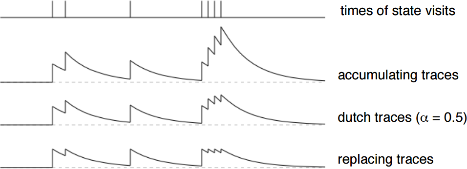
Figure 2.1: Accumulating, Dutch, and replacing eligibility traces (Sutton and Barto [25]).

Using the SARSA update rule in Equation 2.6 yields an algorithm known as TD($\lambda$), while using the Q-Learning update rule yields Q($\lambda$).

Eligibility traces bridge the gap between Monte-Carlo methods and temporal difference methods: With $\lambda=0$, we only consider the current transition, and with $\lambda=1$, we consider the entire episode.

2.6.1 Function Approximation

Until now, we did not specify how to represent $\widehat{Q}$. While we could use a lookup table, in practice, we usually employ a function approximator to address large state spaces (Section 3.1).

In literature, gradient-based function approximation is applied commonly. Using a derivable function approximator like linear regression or neural networks that start from randomly initialized parameters $\theta_{0}$, we can perform the gradient-based update rule:

$$\theta_{t+1}=\theta_{t}+\alpha\delta_{t}\nabla_{\theta}\widehat{Q}(s_{t},a_{t}).$$ (2.7)

Here, $\delta_{t}$ is the scalar offset of the new estimate from the previous one given by the temporal difference error of an algorithm like SARSA or Q-Learning, and $\alpha$ is a small learning rate. Background in function approximation using neural networks is out of the scope of this work.

2.7 Policy-Based Methods

In contrast to value-based methods, policy-based methods parameterize the policy directly. Depending on the problem, finding a good policy can be easier than approximating the Q-function first. Using a parameterized function approximator (Section 2.6.1), we aim to find a good set of parameters $\theta$ such that actions sampled from the policy $a\sim\pi_{\theta}(a_{t},s_{t})$ maximize the reward in a POMDP.

Several methods for searching the space of possible policy parameters have been explored, including random search, evolutionary search , and gradient-based search [6]. In the following, we focus on gradient-based methods.

The PolicyGradient algorithm is the most basic gradient-based method for policy search. The idea is to use the reward signals as objective and tweak the parameters $\theta_{t}$ using gradient ascent. For this to work, we are interested in the gradient of the expected reward under the policy with respect to its parameters:

$$\nabla_{\theta}\rm I\kern-3.00003pt\mathbb{E}_{\pi_{\theta}}\left[R_{t}\right]=\nabla_{\theta}\sum_{s\in S}{d^{\pi_{\theta}}(s)\sum_{a\in A}{\pi_{\theta}(a|s)R_{t}}}$$

where $d^{\pi_{\theta}}(s)$ denotes the probability of being in state $s$ when following $\pi_{\theta}$. Of course, we cannot find that gradient analytically because the agent interacts with an unknown, usually non-differentiable, environment. However, it is possible to obtain an estimate of the gradient using the score-function gradient estimator [26]:

$$\nabla_{\theta}\rm I\kern-3.00003pt\mathbb{E}_{\pi_{\theta}}\left[R_{t}\right] =\nabla_{\theta}\sum_{s_{t}\in S}{d^{\pi_{\theta}}\sum_{a_{t}\in A}{\pi_{\theta}(a|s)R_{t}}}$$ (2.8)

$$=\sum_{s_{t}\in S}{d^{\pi_{\theta}}\sum_{a_{t}\in A}{\nabla_{\theta}\pi_{\theta}(a_{t}|s_{t})R_{t}}}$$

$$=\sum_{s_{t}\in S}{d^{\pi_{\theta}}\sum_{a_{t}\in A}{\pi_{\theta}(a_{t}|s_{t})\frac{\nabla_{\theta}\pi_{\theta}(a_{t}|s_{t})}{\pi_{\theta}(a_{t}|s_{t})}R_{t}}}$$

$$=\sum_{s_{t}\in S}{d^{\pi_{\theta}}\sum_{a_{t}\in A}{\pi_{\theta}(a_{t}|s_{t})\nabla_{\theta}\ln(\pi_{\theta}(a_{t}|s_{t}))R_{t}}}$$

$$=\rm I\kern-3.00003pt\mathbb{E}_{\pi_{\theta}}\left[R_{t}\nabla_{\theta}\ln\pi_{\theta}(a_{t}|s_{t})\right],$$

where we decompose the expectation into a weighted sum following the definition of the expectation and move the gradient inside the sum. We then both multiply and divide the term inside the sum by $\pi_{\theta}(a|s)$, apply the chain rule $\nabla_{\theta}\ln(f(\theta))=\frac{1}{f(\theta)}\nabla_{\theta}f(\theta)$, and bring the result back into the form of an expectation.

As shown in Equation 2.8, we only require the gradient of our policy. Using a derivable function approximator, we can then sample trajectories from the environment to obtain a Monte-Carlo estimate both over states and Equation 2.8. This yields the Reinforce algorithm proposed by Williams [33].

As for value-based methods, the Monte-Carlo estimate is comparatively slow because we only update our estimates at the end of each episode. To improve on that, we can combine this approach with eligibility traces (Section 2.6). We can also reduce the variance of the Monte-Carlo estimates as described in the next section.

2.8 Actor-Critic Methods

In the previous section, we trained the policy along the gradient of the expected reward, that is equivalent to $\rm I\kern-3.00003pt\mathbb{E}_{\pi_{\theta}}\left[R_{t}\nabla_{\theta}\ln\pi_{\theta}(a|s)\right]$. When we sample transitions from the environment to estimate this expectation, the rewards can have a high variance. Thus, Reinforce requires many transitions to obtain a sufficient estimate.

Actor-critic methods improve on the data efficiency of this algorithm by subtracting a baseline $B(s)$ from the reward that reduces the variance of the expectation. When $B(s)$ is an approximated function, we call its approximator critic and the approximator of the policy function actor. To not introduce bias to the gradient of the reward, the gradient of the baseline with respect to the policy must be $0$ [33]:

$$\rm I\kern-3.00003pt\mathbb{E}_{\pi_{\theta}}\left[\nabla_{\theta}\ln\pi_{\theta}(a|s)B(s)\right] =\sum_{s\in S}{d^{\pi_{\theta}}(s)\sum_{a\in A}{\nabla_{\theta}\pi_{\theta}(a|s)B(s)}}$$

$$=\sum_{s\in S}{d^{\pi_{\theta}}(s)B(s)\nabla_{\theta}\sum_{a\in A}{\pi_{\theta}(a|s)}}$$

$$=0.$$

A common choice is $B(s)\approx V^{\pi}(s)$. In this case, we train the policy by the gradient $\rm I\kern-3.00003pt\mathbb{E}_{\pi_{\theta}}\left[\nabla_{\theta}\ln\pi_{\theta}(a|s)(R_{t}-V_{t}(s_{t}))\right]$. Here we can train the critic to approximate $V(s_{t})$ using familiar temporal difference methods (Section 2.5). This algorithm is known as AdvantageActorCritic as $R_{t}-V_{t}(s_{t})$ estimates the advantage function $Q(s_{t},a_{t})-V(s_{t})$ that describes how good an action is compared to how good the average action is in the current state.

Chapter 3 Challenges in Complex Environments

Traditional benchmark problems in RL include tasks like Mountain Car and Cart Pole. In those tasks, the observation and action spaces are small, and the dynamics can be described by simple formulas. Moreover, these environments are usually fully observed so that the agent could reconstruct the system dynamics perfectly, given enough transitions.

In contrast, 3D environments like Doom have complex underlying dynamics and large state spaces that the agent can only partially observe. Therefore, we need more advanced methods to learn successful policies (Chapter 4). We now discuss challenges that arise in complex environments and methods to approach them.

3.1 Large State Space

Doom is a 3D environment where agents observe perspective 2D projections from their position in the world as pixel matrices. Having such a large state space makes tabular versions of RL algorithms intractable. We can adjust those algorithms to the use of function approximators and make them tractable. However, the agent receives tens of thousands of pixels every time step. This is a computational challenge even in the case of function approximation.

Downsampling input images only provides a partial solution to this since we must preserve information necessary for effective control. We would like our agents to find small representations of its observations that are helpful for action selection. Therefore, abstraction from individual pixels is necessary. Convolutional neural networks (CNNs) provide a computationally effective way to learn such abstractions [13].

In comparison to normal fully-connected neural networks, CNNs consist of convolutional layers that learn multiple filters. Each filter is shifted over the whole input or previous layer to produce a feature map. Feature maps can optionally be followed by pooling layers that downsample each feature map individually, using the max or mean of neighboring pixels.

Applying the filters across the whole input or previous layer means that we must only learn a small filter kernel. The number of parameters of this kernel does not depend on the input size. This allows for more efficient computation and faster learning compared to fully-connected networks where a layers adds an amount of parameters that is quadratic in the number of the layer size.

Moreover, CNNs exploit the fact that nearby pixels in the observed images are correlated. For example, walls and other surfaces result in evenly textured regions. Pooling layers help to reduce the dimensionality while keeping information represented small details, when important. This is because each filter learns a high-resolution feature and is downsampled individually.

3.2 Partial Observability

In complex environments, observations do no fully reveal the state of the environment. The perspective view that the agent observes in the Doom environment contains reduced information in multiple ways:

• The agent can only look in forward direction and its field of view only includes a fraction of the whole environment.

• Obstacles like walls hide the parts of the scene behind them.

• The perspective projection loses information about the 3D geometry of the scene. Reconstructing the 3D geometry and thus positions of objects is not trivial and might not even have a unique solution.

• Many 3D environments include basic physics simulations. While the agent can see the objects in its view, the pixels do not directly contain information about velocities. It might be possible to infer them, however.

• Several other temporal factors are not represented in the current image, like whether an item or enemy in another room still exists.

To learn a good policy, the agent has to detect spatial and temporal correlations in its input. For example, it would be beneficial to know the position of objects and the agent itself in the 3D environment. Knowing the positions and velocities of enemies would certainly help aiming.

Using hierarchical function approximators like neural networks allows learning high-level representations like the existence of an enemy in the field of view. For high-level representations, neural networks need more than one layer because a layer can only learn linear combinations of the input or previous layer. Complex features might be impossible to construct from a linear combination of input pixels. Zeiler and Fergus [36] visualize the layers of CNNs and show that they actually learn more abstract features in each layer.

To address the temporal incompleteness of the observations, we can use frame skipping, where we collect multiple images and show this stack as one observation to the agent. The agent then decides for an action we repeat while collecting the next stack of inputs [13].

It is also common to use recurrent neural networks (RNNs) [8, 14] to address the problem of partial observability. Neurons in these architectures have self-connections that allow activations to span multiple time steps. The output of an RNN is a function of the current input and the previous state of the network itself. In particular, a variant called Long Short-Term Memory (LSTM) and its variations like Gated Recurrent Unit (GRU) have proven to be effective in a wide range of sequential problems [12].

Combining CNNs and LSTMs, Oh et al. [16] were able to learn useful representations from videos, allowing them to predict up to $100$ observations in the Atari domain (Figure 3.1).

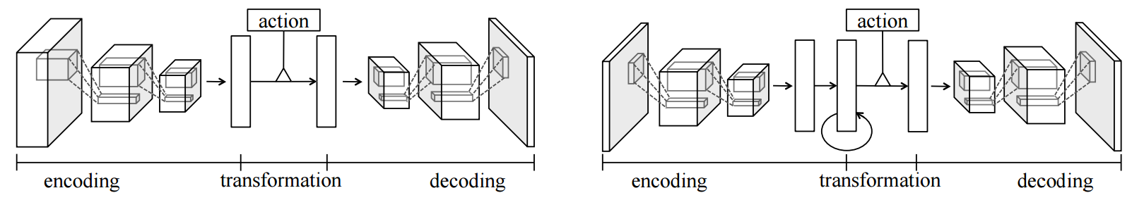
Figure 3.1: Two neural network architectures for learning representations in POMDPs that were used for predicting future observations in Atari. (From Oh et al. [16])

A recent advancement was applying memory network architectures [32, 7] to RL problems in the Minecraft environment [17]. These approximators consist of an RNN that can write to and read from an external memory. This allows the network to clearly carry information over long durations.

3.3 Stable Function Approximation

Various forms of neural networks have been successfully applied to supervised and unsupervised learning problems. In those applications, the dataset is often known prior to training and can be decorrelated and many machine learning algorithms expect independent and identically distributed data. This is problematic in the RL setting, where we want to improve the policy while collecting observations sequentially. The observations can be highly correlated due to the sequential nature underlying the MDP.

To decorrelate data, the agent can use a replay memory as introduced by Mnih et al. [13] to store previously encountered transitions. At each time step, the agent then samples a random batch of transitions from this memory and uses this for training. To initialize the memory, one can run a random policy before the training phase. Note that the transitions are still biased by the start distribution of the MDP.

The mentioned work first managed to learn to play several 2D Atari games [3] without the use of hand-crafted features. It has also been applied to simple tasks in the Minecraft [2] and Doom [9] domains. On the other hand, the replay memory is memory intense and can be seen as unsatisfyingly far from the way humans process information.

In addition, Mnih et al. [13] used the idea of a target network. When training approximators by bootstrapping (Section 2.5), the targets are estimated by the same function approximator. Thus, after each training step, the target computation changes which can prevent convergence as the approximator is trained toward a moving target. We can keep a previous version of the approximator to obtain the targets. After every few time steps, we update the target network by the current version of the training approximator.

Recently, Mnih et al. [14] proposed an alternative to using replay memories that involves multiple versions of the agent simultaneously interacting with copies of the environment. The agents apply gradient updates to a shared set of parameters. Collecting data from multiple environments at the same time sufficiently decorrelated data to learn better policies than replay memory and target network were able to find.

3.4 Sparse and Delayed Rewards

The problem of non-informative feedback is not tied to 3D environments in particular, yet constitutes a significant challenge. Sometimes, we can help and guide the agent by rewarding all actions with positive or negative rewards. But in many real-world tasks, the agent might receive zero rewards most of the time and only see a binary feedback at the end of each episode.

Rare feedback is common when hand-crafting a more informative reward signal is not straightforward, or when we do not want to bias the solutions that the agent might find. In these environments, the agent has to assign credit among all its previous actions when finally receiving a reward.

We can apply eligibility traces (Section 2.6) to function approximation by keeping track of all transitions since the start of the episode. When the agent receives a reward, it incorporates updates for all stored states relative to the decayed reward.

Another way to address sparse and delayed rewards is to employ methods of temporal abstraction as explained in Section 3.5.4

3.5 Efficient Exploration

Algorithms like Q-Learning (Section 2.5) are optimal in the tabular case under the assumption that each state will be visited over and over again, eventually [29]. In complex environments, it is impossible to visit each of the many states. Since we use function approximation, the agent can already generalize between similar states. There are several paradigms to the problem of effectively finding interesting and unknown experiences that help improve the policy.

3.5.1 Random Exploration

We can use a simple EpsilonGreedy strategy for exploration, where at each time step, with a probability of $\varepsilon\in\left(0,1\right]$, we choose a completely random action, and act according to our policy otherwise. When we start at $\varepsilon=1$ and exponentially decay $\varepsilon$ over time, this strategy, in the limit, guarantees to visit each state over and over again.

In simple environments, EpsilonGreedy might actually visit each state often enough to derive the optimal policy. But in complex 3D environments, we do not even visit each state once in a reasonable time. Visiting novel states would be important to discover better policies.

One reason that random exploration still works reasonably well in complex environments [13, 14] can partly be attributed to function approximation. When the function approximator generalizes over similar states, visiting one state also improves the estimate of similar states. However, more elaborate methods exist and can result in better results.

3.5.2 Optimism in the Face of Uncertainty

A simple paradigm to encourage exploration in value-based algorithms (Section 2.2) is to optimistically initialize the estimated Q-values. We can do this either by pre-training the function approximator or by adding a positive bias to its outputs. Whenever the agent visits an unknown state, it will correct its Q-value downward. Less visited states still have high values assigned so that the agent tends to visiting them when facing the choice.

The Bayesian approach is to count the visits of each state to compute the uncertainty of its value estimate [24]. Combined with Q-learning, this converges to the true Q-function, given enough random samples [11]. Unfortunately, it is hard to obtain truly random samples for a general MDP because of its sequential nature. Another problem of counting is that the state space may be large or continuous and we want to generalize between similar states.

Bellemare et al. [4] recently suggested a sequential density estimation model to derive pseudo-counts for each state in a non-tabular setting. Their method significantly outperforms existing methods on some games of the Atari domain, where exploration is challenging.

We can also use uncertainty-based exploration with policy gradient methods (Section 2.7). While we usually do not estimate the Q-function here, we can add the entropy of the policy as a regularization term to the its gradient [34] with a small factor $\beta\in\mathbb{R}$ specifying the amount of regularization:

$$\begin{gathered}\rm I\kern-3.00003pt\mathbb{E}_{\pi_{\theta}}\left[R(s,a)\nabla_{\theta}\log\pi_{\theta}(a|s)\right]+\beta\nabla_{\theta}\mathbb{H}\big{(}\pi_{\theta}(a|s)\big{)},with\\ \mathbb{H}\big{(}\pi_{\theta}(a|s)\big{)}=-\sum_{a^{\prime}\in A}{\pi_{\theta}(a^{\prime}|s)}\log\pi_{\theta}(a^{\prime}|s).\end{gathered}$$ (3.1)

This encourages a uniformly distributed policy until the policy gradient updates outweigh the regularization. The method was successfully applied to Atari and a visual 3D domain Labyrinth by Mnih et al. [14].

3.5.3 Curiosity and Intrinsic Motivation

A related paradigm is to explore in order to attain knowledge about the environment in the absence of external rewards. This usually is a model-based approach that directly encourages novel states based on two function approximators.

The first approximator, called model, tries to predict the next observation and thus approximates the transition function of the MDP. The second approximator, called controller, performs control. Its objective is both to maximize expected returns and to cause the highest reduction in prediction error of the model [19]. It therefore tries to provide new observations to the model that are novel but learnable, inspired by the way humans are bored by both known knowledge and knowledge they cannot understand [20].

The model-controller architecture has been extended in multiple ways. Ngo et al. [15] combined it with planning to escape known areas of the state space more effectively. Schmidhuber [21] recently proposed shared neurons between the model and controller networks in a way that allows the controller to arbitrarily exploit the model for control.

3.5.4 Temporal Abstraction

While most RL algorithms directly produce an action at each time step, humans plan actions on a slower time scale. Adapting this property might be necessary for human level control in complex environments. Most of the mentioned exploration methods (Section 3.5) determine the next exploration action at each time step. Temporally extended actions could be beneficial to both exploration and exploitation [18].

The most common framework for temporal abstraction in the RL literature is the options framework proposed by Sutton et al. [27]. The idea is to learn multiple low-level policies, named options, that interact with the world. A high-level policy observes the same inputs but has the options as actions to choose from. When the high-level policy decides for an option, the corresponding low-level policy is executed for a fixed or random number of time steps.

While there are multiple ways to obtain options, two recent approaches were shown to work in complex environments. Krishnamurthy et al. [10] used spectral clustering to group states with cluster centers representing options. Instead of learning individual low-level policies, the agent greedily follows a distance measure between low-level states and cluster centers that is given by the clustering algorithm.

Also building on the options framework, Tessler et al. [28] trained multiple CNNs on simple tasks in the Minecraft domain. These so-called deep skill networks are added in addition to the low-level actions for the high-level policy to choose from. The authors report promising results on a navigation task.

A limitation of the options framework is its single level of hierarchy. More realistically, multi-level hierarchical algorithms are mainly explored in the fields of cognitive science and computational neuroscience. Rasmussen and Eliasmith [18] propose one such architecture and show that it is able to learn simple visual tasks.

Chapter 4 Algorithms for Learning from Pixels

We explained the background of RL methods in Chapter 2 and described the challenges that arise in complex environments in Chapter 3, where we already outlined the intuition behind some of the current algorithms. In this section, we build on this and explain two state-of-the-art algorithms that have successfully been applied to 3D domains.

4.1 Deep Q-Network

The currently most common algorithm for learning in high-dimension state spaces is the Deep Q-Network (DQN) algorithm suggested by Mnih et al. [13]. It is based on traditional Q-Learning algorithm with function approximation and EpsilonGreedy exploration. In its initial form, DQN does not use eligibility traces.

The algorithm uses a two-layer CNN, followed by a linear fully-connected layer to approximate the Q-function. Instead of taking both state and action as input, it outputs the approximated Q-values for all actions $a\in A$ simultaneously, taking only a state as input.

To decorrelate transitions that the agent collects during play, it uses a large replay memory. After each time step, we select a batch of transitions from the replay memory randomly. We use the temporal difference Q-Learning rule to update the neural network. We initialize $\varepsilon=1$ and start annealing it after the replay memory is filled.

In order to further stabilize training, DQN uses a target network to compute the temporal difference targets. We copy the weights of the primary network to the target network at initialization and after every few time steps. As initially proposed, the algorithms synchronizes the target network every frame, so that the targets are computed using the network weights at the last time step.

DQN has been successfully applied to two tasks within the Doom domain by Kempka et al. [9] who introduced this domain. In the more challenging Health Gathering task, where the agent must collect health items in multiple open rooms, they used three convolutional layers, followed by max-pooling layers and a fully-connected layer. With a small learning rate of $\alpha=0.00001$, a replay memory of $10000$ entries, and one million training steps, the agent learned a successful policy.

Barron et al. [2] applied DQN to two tasks in the Minecraft domain: Collecting as many blocks of a certain color as possible, and navigating forward on a pathway without falling. In both tasks, DQN learned successful policies. Depending on the width of the pathway, a larger convolutional network and several days of training were needed to learn successful policies.

4.2 Asynchronous Advantage Actor Critic

A3C by Mnih et al. [14] is an actor-critic method that is considerable more memory-efficient than DQN, because it does not require the use of a replay memory. Instead, transitions are decorrelated by training in multiple versions of the same environment in parallel and asynchronously updating a shared actor-critic model. Entropy regularization (Section 3.5.2) is employed to encourage exploration.

Each of the originally up to $16$ threads manages a copy of the model, and interacts with an instance of the environment. Each threads collects a few transitions before computing eligibility returns (Section 2.6) and computing gradients according to the AAC algorithm (Section 2.8) based on its current copy of the model. It then applies this gradient to the shared model and updates its copy to the current version of the shared model.

One version of A3C uses the same network architecture as DQN, except for using a softmax activation function in the last layer to model the policy rather than. The critic model shares all convolutional layers and only adds a linear fully-connected layer of size one that is trained to estimate the value function. The authors also proposed a version named LSTM-A3C that adds one LSTM layer between the convolutional layers and the output layers to approach the problem of partial observability.

In addition to Atari and a continuous control domain, A3C was evaluated on a new Labyrinth domain, a 3D maze where the goal is to find and collect as many apples as possible. LSTM-A3C was able to learn a successful policy for this task that avoids to walk into walls and turns around when facing dead ends. Given the recent proposal of the algorithm, it is not likely that the algorithm was applied to other 3D domains yet.

Chapter 5 Experiments in the Doom Domain

We now introduce the Doom domain in detail, focusing on the task used in the experiments. We explain methods that were necessary to train the algorithms (Chapter 4) in a stable manner. While the agents do not reach particularly high scores on average, they learn a range of interesting behaviors that we examine in Section 5.5.

5.1 The Doom Domain

The Doom domain [9] provides RL tasks simulated by the game mechanics of the first-person shooter Doom. This 3D game features different kinds of enemies, items, and weapons. A level editor can be used to create custom tasks. We use the DeathMatch task defined in the Gym collection [5]. We first describe the Doom domain in general.

In Doom, the agent observes image frames that are perspective 2D projections of the world from the agent’s position. A frame also contains user interface elements at the bottom, including the amount of ammunition of the agent’s selected weapon, the remaining health points of the agent, and additional game-specific information. We do not extract this information explicitly.

Each frame is represented as a tensor of dimensions screen width, screen height, and color channel. We can choose the width and height from a set of available screen resolutions. The color channel represents the RGB values of the pixels and thus always has a size of three.

The actions are arbitrary combinations of the $43$ available user inputs to the game. Most actions are binary values to represent whether a given key on the keyboard is in pressed or released position. Some actions represent mouse movement and take on values in the range $\left[-10,10\right]$ with $0$ meaning no movement.

The available actions perform commands in the game, such as attack, jump, crouch, reload, run, move left, look up, select next weapon, and more. For a detailed list, please refer to the whitepaper by Kempka et al. [9].

We focus on the DeathMatch task, where the agent faces multiple kinds of enemies that attack it. The agent must shoot an enemy multiple times, depending on the kind of enemy, to kill it an receive a reward of $+1$. Being hit by enemy attacks reduces the agent’s health points, eventually causing the end of the episode. The agent does not receive any reward the end of the episode. The episode also ends after exceeding $10^{4}$ time steps.

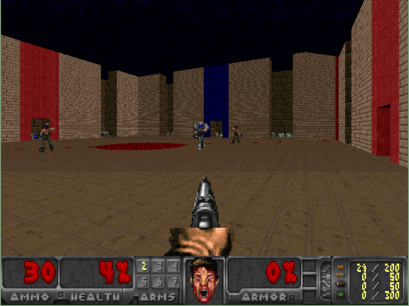
Figure 5.1: The environment of the DeathMatch task contains a hall where enemies appear, and four rooms to the sides. The rooms contain either health items (red entry) or weapons and ammunition (blue entry).

As shown in Figure 5.1, the world consists of one large hall, where enemies appear regularly, and four small rooms to the sides. Two of the small rooms contain items for the agent to restore health points. The other two rooms contain ammunition and stronger weapons than the pistol that the agent begins with. To collect items, ammunition, or weapons, the agent must walk through them. The agent starts at a random position in the hall, facing a random direction.

5.2 Applied Preprocessing

To reduce computation requirements, we choose the smallest available screen resolution of $160\times 120$ pixels. We further down-sample the observations to $80\times 60$ pixels, and average over the color channels to produce a grayscale image. We experiment with delta frames, where we pass the difference between the current and the last observation to the agent. Both variants are visualized in Figure 5.2.

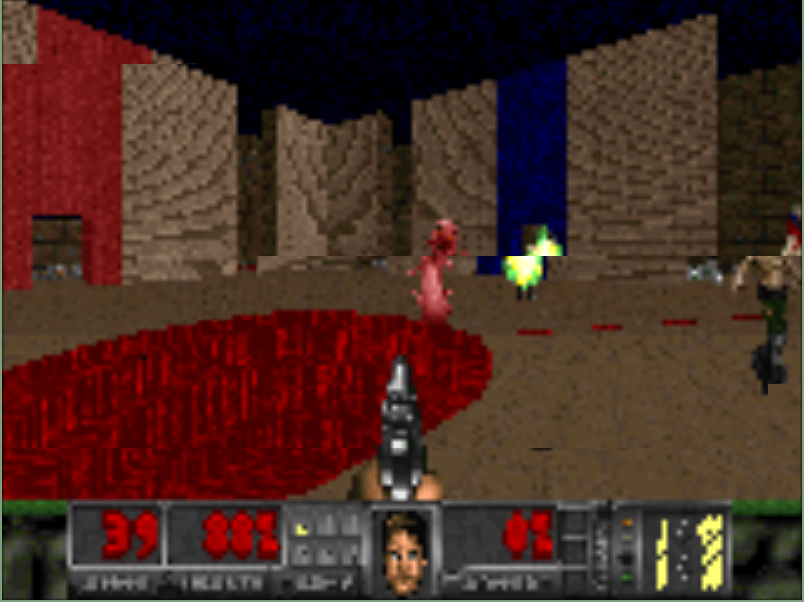
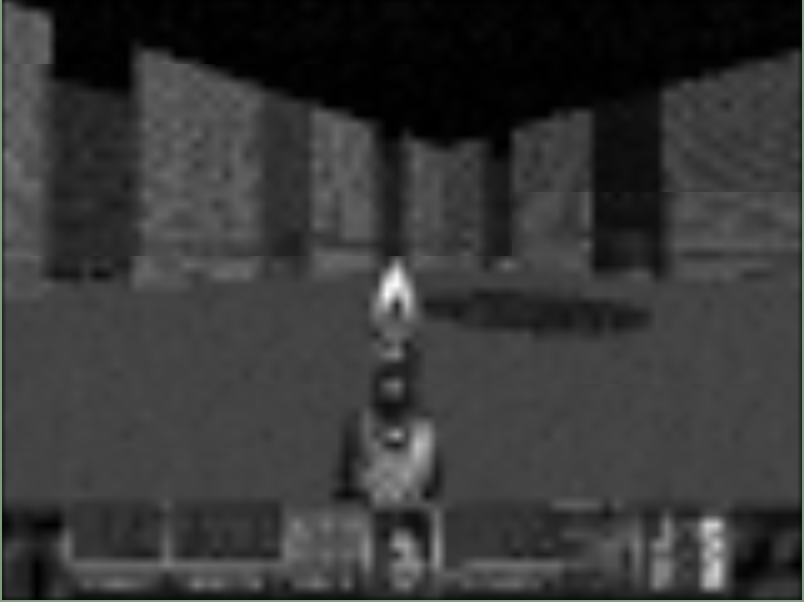
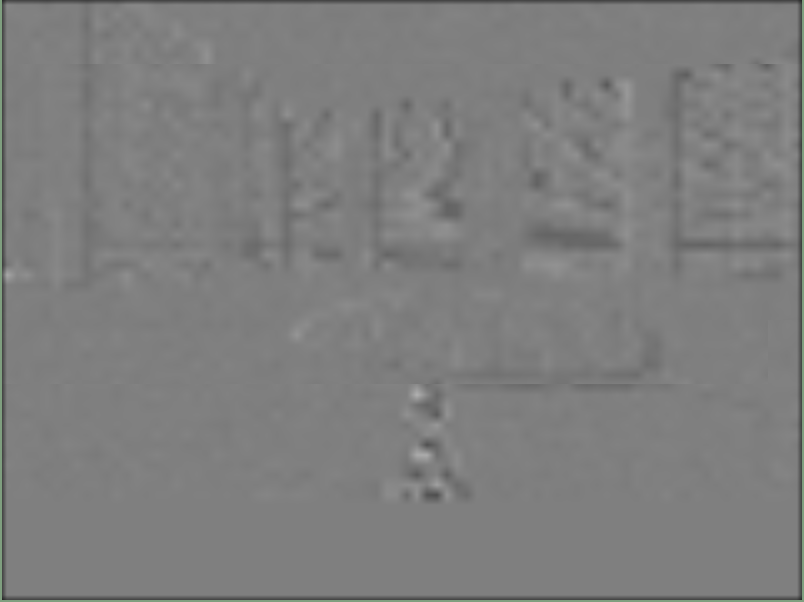
Figure 5.2: Three observations of the DeathMatch task: An unprocessed frame (left), a downsampled grayscale frame (center), and a downsampled grayscale delta frame (right). Based on human testing, both preprocessing methods retain observations sufficient for successful play.

We further employ history frames as originally used by DQN in the Atari domain, and further explored by Kempka et al. [9]. Namely, we collect multiple frames, stack them, and show them to the agent as one observation. We then repeat the agent’s action choice over the next time steps while collecting a new stack of images. We perform a random action during the first stack of an episode. History frames have multiple benefits: They include temporal information, allow more efficient data processing, and cause actions to be extended for multiple time steps, resulting in more smooth behavior.

History frames extend the dimensionality of the observations. We use the grayscale images to compensate for this and keep computation requirements manageable. While color information could be beneficial to the agent, we expect the temporal information contained in history frames to be more valuable, especially to the state-less DQN algorithm. Further experiments would be needed to test this hypothesis.

We remove unnecessary actions from the action space to speed up learning, leaving only the $7$ actions attack, move left, move right, move forward, move backward, turn left, and turn right. Note that we do not include actions to rotate the view upward or downward, so that the agent does not have to learn to look upright.

Finally, we apply normalization: We scale the observed pixels into the range $\left[0,1\right]$ and normalize rewards to $(-1,0,+1)$ using $r_{t}\leftarrow\operatorname{sgn}(r_{t})$ [13]. Further discussion of normalization can be found in the next section.

5.3 Methods to Stabilize Learning

Both DQN and LSTM-A3C are sensitive to the choice of hyper parameters [14, 23]. Because training times lie in the order of hours or days, it is not tractable to perform an excessive hyper parameter search for most researcher. We can normalize observations and rewards as described in the previous section to make it more likely that hyper parameters can be transferred between tasks and domains.

It was found to be essential to clip gradients of the networks in both DQN and LSTM-A3C. Without this step, the approximators diverges in the early phase of learning. Specifically, we set each element $x$ of the gradient to $x\leftarrow\max\left\{-10,\min\left\{x,+10\right\}\right\}$. The exact threshold to clip at did not seem to have a large impact on training stability or results.

We decay the learning rate linearly over the course of training to guarantee convergence, as done by Mnih et al. [13, 14], but not by Kempka et al. [9], Barron et al. [2].

5.4 Evaluation Methodology

DQN uses a replay memory of the last $10^{4}$ transitions and samples batches of size $64$ from it, following the choices by Kempka et al. [9]. We anneal $\varepsilon$ from $1.0$ to $0.1$ over the course of $2*10^{6}$ time steps, which is one third of the training duration. We start both training and annealing $\varepsilon$ after the first $10^{4}$ observations. This is equivalent to initializing the replay memory from transitions collected by a random policy.

For LSTM-A3C, we use $16$ learning threads that apply their accumulated gradients every $5$ observations using shared optimizer statistics, a entropy regularization factor of $\beta=0.01$. Further, we scale the loss of the critic by $0.5$ [14].

Both algorithms operate on frames of history $6$ at a time and use RMSProp with a decay parameter of $0.99$ for optimization [14]. The learning rate starts at $\alpha=2*10^{-5}$, similar to Kempka et al. [9] who use a fixed learning rate of $10^{-5}$ in the Doom domain.

We train both algorithms for $20$ epochs, where one epoch corresponds to $5*10^{4}$ observations for DQN and $8*10^{5}$ observations for LSTM-A3C, resulting in comparable running times of both algorithms. After each epoch, we evaluate the learned policies on $10^{4}$ or $10^{5}$ observations, respectively. We measure the score, that is, the sum of collected rewards, that we average over the training episodes. DQN uses $\varepsilon=0.05$ during evaluation.

5.5 Characteristics of Learned Policies

In the conducted experiments, both algorithms were able to learn interesting policies during the $20$ epochs. We describe and discuss instances of such policies in this section. The results of DQN and LSTM-A3C are similar in many cases, suggesting that both algorithms discover common structures of the DeathMatch task.

The agents did not show particular changes when receiving delta frames (Section 5.2) as inputs. This might be because given history frames, neural networks can easily learn to compute differences between those frames if useful to solve the task. Therefore, we conclude that delta frames may not be useful in combination with history frames.

5.5.1 Fighting Against Enemies

As expected, the agents develop a tendency to aim at enemies. Because an agent needs to directly look toward enemies in order to shoot them, it always faces an enemy the time step before receiving a positive reward. However, the aiming is inaccurate and the agents tend to look past their enemies to the left and right side, alternatingly. It would be interesting to conduct experiments without stacking history frames to understand whether the learned policies are limited by the action repeat.

In several instances, the agents lose enemies from their field of view by turning, usually toward other enemies. No trained agent was found to memorize such enemies after not seeming them anymore. As a result, the agents were often attacked from the back, causing the episode to end.

Surprisingly, LSTM-A3C agents tend to only attack when facing an enemy, but sometimes miss out the chance to do so. In contrast, DQN agents were found to shoot regularly and more often than LSTM-A3C. Further experiments would be needed to verify, whether this behavior persists after training for more than $20$ episodes.

5.5.2 Navigation in the World

Most agents learn to avoid running into walls while facing them, suggesting at least a limited amount of spatial awareness. In comparison, a random agent repeatedly runs into a wall and gets stuck in this position until the end of the episode.

In some instances, the agent walks backward against a wall at an angle, so that it slides along the wall until reaching the entrance of a side room. This behavior overfits to the particular environment of the DeathMatch task, but represents a reasonable policy to pick up the more powerful weapons inside two of the side rooms. We did not find testing episodes in which the agent used this strategy to enter one of the rooms containing health restoring items. This could be attributed to the lack of any negative reward when the agent dies.

Notably, in one experiment, LSTM-A3C agent collects the rocket launcher weapon using this wall-sliding strategy, and starts to fire after collecting it. The agents did not fire before collecting that weapon. During training, there might have been successful episodes, where the agent initially collected this weapon. Another reason for this could be that the first enemies only appear after a couple of time steps so there is no reason to fire in the beginning of an episode.

In general, both tested algorithms, DQN and LSTM-A3C, were able to learn interesting policies for our task in the Doom domain in relatively short amounts of training time. On the other hand, the agents did not find ways to effectively shoot multiple enemies in a row. An evaluation over multiple choices of hyper parameters and longer training times would be a sensible next step.

Chapter 6 Conclusions

We started by introducing reinforcement learning (RL) and summarized basic reinforcement learning methods. Compared to traditional benchmarks, complex 3D environments can be more challenging in many ways. We analyze these challenges and review current algorithms and ideas to approach these.

Following this background, we select to algorithms that were successfully applied to learn from pixels in 3D environments. We apply both algorithms to a challenging task within the recently presented Doom domain, that is based on a 3D first-person-shooter game.

Applying the selected algorithms yields policies that do not reach particularly high scores, but show interesting behavior. The agents tend to aim at enemies, avoid getting stuck in walls, and find surprising strategies within this Doom task.

We also assess that using delta frames does not affect the training much when combined with stacking multiple images together as input to the agent. In would be interesting to see if using fewer action repeats allows for more accurate aiming.

The drawn conclusions are not final because other hyper parameters or longer training might allow these algorithms to perform better. We analyze instances of learned behavior and believe that observations reported in the work provide a valuable starting point for further experiments in the Doom domain.

Declaration of Authorship

I hereby declare that the thesis submitted is my own unaided work. All direct or indirect sources used are acknowledged as references.

Potsdam, March 8, 2024

Danijar Hafner

References

- Abbeel et al. [2007] P. Abbeel, A. Coates, M. Quigley, and A. Y. Ng. An application of reinforcement learning to aerobatic helicopter flight. Advances in neural information processing systems, 19:1, 2007.
- Barron et al. [2016] T. Barron, M. Whitehead, and A. Yeung. Deep reinforcement learning in a 3-d blockworld environment. In Deep Reinforcement Learning: Frontiers and Challenges, IJCAI 2016, 2016.
- Bellemare et al. [2012] M. G. Bellemare, Y. Naddaf, J. Veness, and M. Bowling. The arcade learning environment: An evaluation platform for general agents. Journal of Artificial Intelligence Research, 2012.
- Bellemare et al. [2016] M. G. Bellemare, S. Srinivasan, G. Ostrovski, T. Schaul, D. Saxton, and R. Munos. Unifying count-based exploration and intrinsic motivation. arXiv preprint arXiv:1606.01868, 2016.
- Brockman et al. [2016] G. Brockman, V. Cheung, L. Pettersson, J. Schneider, J. Schulman, J. Tang, and W. Zaremba. Openai gym, 2016.
- Deisenroth et al. [2013] M. P. Deisenroth, G. Neumann, J. Peters, et al. A survey on policy search for robotics. Foundations and Trends in Robotics, 2(1-2):1–142, 2013.
- Graves et al. [2014] A. Graves, G. Wayne, and I. Danihelka. Neural turing machines. arXiv preprint arXiv:1410.5401, 2014.
- Hausknecht and Stone [2015] M. Hausknecht and P. Stone. Deep recurrent q-learning for partially observable mdps. arXiv preprint arXiv:1507.06527, 2015.
- Kempka et al. [2016] M. Kempka, M. Wydmuch, G. Runc, J. Toczek, and W. Jaśkowski. Vizdoom: A doom-based ai research platform for visual reinforcement learning. CoRR, 2016.
- Krishnamurthy et al. [2016] R. Krishnamurthy, A. S. Lakshminarayanan, P. Kumar, and B. Ravindran. Hierarchical reinforcement learning using spatio-temporal abstractions and deep neural networks. arXiv preprint arXiv:1605.05359, 2016.
- Li [2009] L. Li. A unifying framework for computational reinforcement learning theory. PhD thesis, Rutgers, The State University of New Jersey, 2009.
- Lipton et al. [2015] Z. C. Lipton, J. Berkowitz, and C. Elkan. A critical review of recurrent neural networks for sequence learning. arXiv preprint arXiv:1506.00019, 2015.
- Mnih et al. [2013] V. Mnih, K. Kavukcuoglu, D. Silver, A. Graves, I. Antonoglou, D. Wierstra, and M. Riedmiller. Playing atari with deep reinforcement learning. In 5602, 2013.
- Mnih et al. [2016] V. Mnih, A. P. Badia, M. Mirza, A. Graves, T. P. Lillicrap, T. Harley, D. Silver, and K. Kavukcuoglu. Asynchronous methods for deep reinforcement learning. In Proceedings of the 33rd International Conference on Machine Learning, 2016.
- Ngo et al. [2013] H. Ngo, M. Luciw, A. Förster, and J. Schmidhuber. Confidence-based progress-driven self-generated goals for skill acquisition in developmental robots. Frontiers in Psychology, 4:833, 2013.
- Oh et al. [2015] J. Oh, X. Guo, H. Lee, R. L. Lewis, and S. Singh. Action-conditional video prediction using deep networks in atari games. In Advances in Neural Information Processing Systems, pages 2863–2871, 2015.
- Oh et al. [2016] J. Oh, V. Chockalingam, S. Singh, and H. Lee. Control of memory, active perception, and action in minecraft. CoRR, abs/1605.09128, 2016.
- Rasmussen and Eliasmith [2014] D. Rasmussen and C. Eliasmith. A neural model of hierarchical reinforcement learning. In Proceedings of the 36th Annual Conference of the Cognitive Science Society, pages 1252–1257. Cognitive Science Society Austin, TX, 2014.
- Schmidhuber [1991] J. Schmidhuber. A possibility for implementing curiosity and boredom in model-building neural controllers. In From animals to animats: proceedings of the first international conference on simulation of adaptive behavior. Citeseer, 1991.
- Schmidhuber [2010] J. Schmidhuber. Formal theory of creativity, fun, and intrinsic motivation (1990–2010). IEEE Transactions on Autonomous Mental Development, 2(3):230–247, 2010.
- Schmidhuber [2015] J. Schmidhuber. On learning to think: Algorithmic information theory for novel combinations of reinforcement learning controllers and recurrent neural world models. arXiv preprint arXiv:1511.09249, 2015.
- Shteingart and Loewenstein [2014] H. Shteingart and Y. Loewenstein. Reinforcement learning and human behavior. Current opinion in neurobiology, 25:93–98, 2014.
- Sprague [2015] N. Sprague. Parameter selection for the deep q-learning algorithm. In Proceedings of the Multidisciplinary Conference on Reinforcement Learning and Decision Making (RLDM), 2015.
- Strens [2000] M. Strens. A bayesian framework for reinforcement learning. In ICML, pages 943–950, 2000.
- Sutton and Barto [1998] R. S. Sutton and A. G. Barto. Reinforcement learning: An introduction, volume 1. MIT press Cambridge, 1998.
- Sutton et al. [1999a] R. S. Sutton, D. A. McAllester, S. P. Singh, Y. Mansour, et al. Policy gradient methods for reinforcement learning with function approximation. In NIPS, volume 99, pages 1057–1063, 1999a.
- Sutton et al. [1999b] R. S. Sutton, D. Precup, and S. Singh. Between mdps and semi-mdps: A framework for temporal abstraction in reinforcement learning. Artificial intelligence, 112(1):181–211, 1999b.
- Tessler et al. [2016] C. Tessler, S. Givony, T. Zahavy, D. J. Mankowitz, and S. Mannor. A deep hierarchical approach to lifelong learning in minecraft. arXiv preprint arXiv:1604.07255, 2016.
- Tsitsiklis [1994] J. N. Tsitsiklis. Asynchronous stochastic approximation and q-learning. Machine Learning, 16(3):185–202, 1994.
- Vamvoudakis and Lewis [2010] K. G. Vamvoudakis and F. L. Lewis. Online actor–critic algorithm to solve the continuous-time infinite horizon optimal control problem. Automatica, 46(5):878–888, 2010.
- Watkins and Dayan [1992] C. J. Watkins and P. Dayan. Q-learning. Machine learning, 8(3-4):279–292, 1992.
- Weston et al. [2014] J. Weston, S. Chopra, and A. Bordes. Memory networks. arXiv preprint arXiv:1410.3916, 2014.
- Williams [1992] R. J. Williams. Simple statistical gradient-following algorithms for connectionist reinforcement learning. Machine learning, 8(3-4):229–256, 1992.
- Williams and Peng [1991] R. J. Williams and J. Peng. Function optimization using connectionist reinforcement learning algorithms. Connection Science, 3(3):241–268, 1991.
- Wymann et al. [2013] B. Wymann, C. Dimitrakakis, A. Sumner, E. Espié, C. Guionneau, and R. Coulom. TORCS, the open racing car simulator, v1.3.5. http://www.torcs.org, 2013.
- Zeiler and Fergus [2014] M. D. Zeiler and R. Fergus. Visualizing and understanding convolutional networks. In European Conference on Computer Vision, pages 818–833. Springer, 2014.