A Chiral Solution to the Ginsparg-Wilson Equation

Abstract

We present a chiral solution of the Ginsparg-Wilson equation. This work is motivated by our recent proposal for nonperturbatively regulating chiral gauge theories, where five-dimensional domain wall fermions couple to a four-dimensional gauge field that is extended into the extra dimension as the solution to a gradient flow equation. Mirror fermions at the far surface decouple from the gauge field as if they have form factors that become infinitely soft as the distance between the two surfaces is increased. In the limit of an infinite extra dimension we derive an effective four-dimensional chiral overlap operator which is shown to obey the Ginsparg-Wilson equation, and which correctly reproduces a number of properties expected of chiral gauge theories in the continuum.

I Introduction

Defining a nonperturbative regulator for chiral gauge theories has been a long-standing problem in quantum field theory. While it may be that finding a regulator is just a technical issue, one should be open to the possibility that its resolution could entail new physics – either in the form of new particles or interactions, or through elucidation of some of the outstanding puzzles of the Standard Model, such as the strong CP problem. The difficulty in constructing a regulator comes down to defining a discretized version of the Euclidian fermion kinetic operator ${\cal D}$ for Weyl fermions in a complex representation of the gauge group, where $\det{\cal D}$ is the fermion contribution to the integration measure for the gauge field path integral. The naive target for the lattice theory is the kinetic operator $\not{D}P_{-}$ , where $D_{\mu}$ is the gauge covariant derivative and $P_{\pm}=(1\pm\gamma_{5})/2$. However, as has been discussed extensively in the literature, while the modulus of this determinant is given by the square root of the Dirac determinant, $|\det{\cal D}|=\sqrt{\det\not{D}}$, its phase is not well-defined. The ambiguity in the phase arises because the operator ${\cal D}$ maps negative chirality spinors into positive chirality spinors and therefore its eigenvalues cannot be uniquely defined. As the negative and positive chirality Hilbert spaces are independent, redefining each basis by an unrelated phase redefines the determinant by a phase which is an arbitrary functional of the gauge field (although most choices of phase could not result from a local fermion action). Furthermore, the phase of the determinant is only gauge-invariant when a theory has no gauge anomalies.

A definition of the Euclidian chiral determinant in the continuum was proposed in Ref. Alvarez-Gaume and Ginsparg (1984), where the authors introduced neutral spectators of opposite chirality, so that that ${\cal D}=\not{\partial}+i\not{A}P_{-}$, which in a chiral representation looks like

$${\cal D}=\begin{pmatrix}\ &D_{\mu}\sigma_{\mu}\\ \partial_{\mu}\bar{\sigma}_{\mu}&\end{pmatrix}\ ,$$ (1)

with $\sigma_{\mu}=\{1,-i\vec{\sigma}\}$, $\bar{\sigma}_{\mu}=\sigma_{\mu}^{\dagger}$. While this form of ${\cal D}$ is not self-adjoint, it does have a well-defined eigenvalue problem and its determinant can be uniquely determined Alvarez-Gaume et al. (1986).

This definition of ${\cal D}$ cannot be directly implemented on the lattice, as is evident when considering the global $U(1)$ chiral anomaly. Chiral symmetry of the fermion action can be expressed by the equation $\{{\cal D},\gamma_{5}\}=0$, or equivalently (in the absence of exact zeromodes) as

$$\left\{{\cal D}^{-1},\gamma_{5}\right\}=0\ .$$ (2)

However, in the continuum the path integral measure cannot be regulated in a way that preserves both gauge and chiral symmetries Fujikawa (1979), which gives rise to the anomalous divergence of the axial current Adler (1969); Bell and Jackiw (1969)

$$\partial_{\mu}j_{\mu}^{5}=\frac{\alpha}{2\pi}{\rm Tr\,}F\widetilde{F}\ .$$ (3)

In contrast, the path integration measure on the lattice is defined in a way that is invariant under both gauge and chiral symmetries. Since it involves only a finite number of degrees of freedom, there are no anomalies and thus no anomalous divergence of the axial current. The correct continuum limit with the axial anomaly can therefore only be attained if the lattice action is not invariant under chiral symmetry transformations. In general such explicit symmetry breaking requires fine tuning to achieve a symmetry that is only broken anomalously in the continuum limit. Additionally at finite lattice spacing, important consequences of chiral symmetry, such as multiplicative mass renormalization, are usually lost. Ginsparg and Wilson argued, however, that by modifying Eq. (2) to read

$$\left\{{\cal D}^{-1},\gamma_{5}\right\}=a\gamma_{5}\ ,$$ (4)

where $a$ is the lattice spacing, chiral symmetry would be broken in just the right way to reproduce the anomaly without fine tuning Ginsparg and Wilson (1982). It was subsequently shown that a solution to the Ginsparg-Wilson equation indeed gives rise to the correct anomaly, while at the same time ensuring an exact symmetry of the action at finite lattice spacing that enforces multiplicative mass renormalization and the absence of fine-tuning Hasenfratz et al. (1998); Luscher (1998). In a chiral basis the general solution to Eq. (4) is

$${\cal D}^{-1}=\begin{pmatrix}0&S_{1}\\ -S_{2}^{\dagger}&0\end{pmatrix}+\frac{a}{2}\begin{pmatrix}1&0\\ 0&1\end{pmatrix}$$ (5)

where each block scales in size with the number of lattice sites, and $S_{1}$, $S_{2}$ can be independent operators; they are constrained by the desired continuum limit and locality, but not by Eq. (4).

The Ginsparg-Wilson equation does not specify whether ${\cal D}$ refers to fermions in a real (Dirac) or complex (chiral) representation of the gauge group. Its solution in the Dirac case is given by the Narayanan-Neuberger overlap operator Narayanan and Neuberger (1994, 1995); Neuberger (1998a, b). In this case $S_{1}={S_{2}}$ and the effect of the diagonal term in ${\cal D}^{-1}$ is very simple. The eigenvalues of the continuum Euclidian Dirac propagator $\not{D}^{-1}$ lie on the imaginary axis while the eigenvalues of ${\cal D}^{-1}$ lie along a parallel line displaced from the imaginary axis by $a/2$; $\not{D}^{-1}$ has an infinite density of eigenvalues approaching the real axis while the lattice propagator ${\cal D}^{-1}$ has a finite density, thanks to the lattice cutoff. The second term on the right side in Eq. (5) is responsible for the $a/2$ displacement and represents the explicit chiral symmetry breaking that is required to reproduce the continuum anomaly.

For a lattice regularization of the target theory given in Eq. (1) – a chiral gauge theory with noninteracting mirror fermions – we would expect that the solution Eq. (5) still pertains, but with $S_{1}\neq{S_{2}}$ and eigenvalues therefore no longer lying on a line parallel to the imaginary axis. However, in this case the chiral symmetry violating part of the solution apparently requires either violating the gauge symmetry explicitly, or else allowing the mirror fermions to participate in the gauge interactions. Either choice is a significant departure from the perturbative scheme. If gauge symmetry is explicitly broken, a path to restoring it in the continuum limit must be devised Golterman and Shamir (2004); if the mirror fermions are gauged, one must understand how to decouple them in the continuum limit. Both strategies have their theoretical challenges, and both have been pursued in the literature; we do not intend to review past work on the subject, but refer the reader to the review Ref. Golterman (2001) as well as the more recent papers Refs. Luscher (2002); Wen (2013); Giedt et al. (2014); You and Xu (2015) and references therein.

The focus of this paper is an alternative approach based on the proposal in Ref. Grabowska and Kaplan (2016). In this theory fermions of one chirality are surface modes on a five-dimensional slab coupling to a gauge field $A$, while their mirror partners of the opposite chirality are modes on the opposite surface coupling to a different gauge field $A_{\star}$. The two gauge fields are related by a gauge-covariant flow equation, where the field $A$ on one surface flows to $A_{\star}$ on the other. In the limit of infinite extra dimension we find a solution to the Ginsparg-Wilson equation of the form Eq. (5) with the continuum limit

$$\lim_{a\to 0}\hat{\cal D}_{\chi}=\begin{pmatrix}0&\sigma_{\mu}D_{\mu}(A)\\ \bar{\sigma}_{\mu}D_{\mu}(A_{\star})&0\end{pmatrix}\ .$$ (6)

Since we only consider gauge-covariant flow equations, the gauge fields $A$ and $A_{\star}$ transform identically under gauge transformations and the diagonal entries of ${\cal D}^{-1}$ at nonzero lattice spacing do not violate gauge invariance. In the limit of infinite extra dimension, $A_{\star}$ is the fixed point of the flow equation given the initial data $A$. We will be interested in two possible scenarios: one where $A_{\star}$ is the classical multi-instanton solution with winding number equal to that of $A$, and the other where $A_{\star}$ is pure gauge, the latter being a possible fixed point for a gauge covariant gradient flow equation on the lattice. In either case, with all dynamical degrees of freedom damped out of $A_{\star}$, one might expect the mirror fermions to entirely decouple in the continuum and infinite volume limits, effectively realizing the continuum construction in Eq. (1).

In the next section we review the proposal of Ref. Grabowska and Kaplan (2016) for five-dimensional fermions coupled to a four-dimensional gauge field, extended into the extra dimension via gradient flow. We then review the technology developed by Narayanan and Neuberger to construct the effective overlap fermion operator for vector-like gauge theories from domain wall fermions with infinite extra dimension Narayanan and Neuberger (1994, 1995); Neuberger (1998a, b). By applying their reasoning to the theory of Ref. Grabowska and Kaplan (2016) we attain the main result of this paper. After discussing the behavior of the chiral overlap operator for gauge fields with nontrivial topology we suggest a simulation to test key ideas presented here.

II Domain wall fermions for chiral gauge theories

Domain wall fermions can be formulated as Dirac fermions in five Euclidean dimensions with masses that depend on the extra dimension. Specifically, consider the coordinate of the extra dimension to be $s\in[-L,L]$, with periodic boundary conditions for a Dirac fermion field which has a positive mass on half the space and a negative mass on the other half Kaplan (1992, 2009); Grabowska and Kaplan (2016). The spectrum contains a light boundstate at each of the two mass defects that behave as a four-dimensional Dirac fermion with a mass which vanishes exponentially fast in the $L\to\infty$ limit; the two boundstates become positive and negative chirality eigenstates respectively in that limit. The domain wall fermion construction provides a solution to the problem of realizing chiral symmetry correctly for lattice fermions in a vector-like representation of the gauge group: (i) the chiral anomaly is correctly realized via the Callan-Harvey effect, where a Chern-Simons operator is generated by integrating out the massive bulk fermions Callan and Harvey (1985), and (ii) any small mass term introduced for the light modes can only be multiplicatively renormalized due to the vanishing wavefunction overlap between the negative and positive chirality fermion modes in the absence of such a mass term. Furthermore the number and chiralities of the light surface modes in the spectrum is a topological invariant of the bulk fermion dispersion relation in momentum space, as shown in Ref. Golterman et al. (1993), and is not simply given by the number of fields in the five-dimensional theory.

An important feature discovered in Refs. Jansen and Schmaltz (1992); Golterman et al. (1993) is that in a regulated theory the contributions to the Chern-Simons current can trivially vanish in half of the bulk, making that region a true insulator. Thus one can take the fermion mass to be infinite on the $s\in(-L,0)$ half space, essentially excising that part of the space, and instead only consider the half-space $s\in[0,L]$, with fermion zeromodes confined to the surfaces of the slab. This gives rise to Shamir’s formulation of domain wall fermions Shamir (1993); Furman and Shamir (1995) which serves as the foundation for practical simulations of lattice QCD.

From the beginning, the physical separation of chiral fermion modes in the extra dimension has been seen as a promising starting point for the construction of chiral gauge theories Kaplan (1992). Multiple flavors of fermions in different representations of the gauge group can be trivially incorporated in the construction, with either chirality localized at a specific surface. Of particular interest are systems where the coefficient of the bulk Chern-Simons operator in the effective theory vanishes due to cancellations between contributions from the different flavors of fermions, eliminating charge exchange between the two surfaces. Such a cancellation is equivalent to the group theoretical statement that the chiral fermions at each surface are independently in a representation that is free from gauge anomalies, and hence each is in its own right a candidate for a healthy four-dimensional gauge theory. Constructions of anomaly cancellation models were examined in the early 1990s Jansen (1992); Kaplan (1992, 1993), the most trivial consisting of two five-dimensional (or three-dimensional) fermions in the same gauge representation but with opposite signs for their masses, rendering the theory $P$- and $T$-invariant, with the zeromode spectrum at each surface consisting of a massless Dirac fermion. Quantum field theories exhibiting less trivial anomaly cancellation were also studied, such as the 3-4-5 $U(1)$ gauge theory in two dimensions Jansen and Schmaltz (1992). Models where the surface modes are Majorana fermions were also constructed for the purpose of simulating supersymmetry, where the massless Majorana fermions serve as gauginos Neuberger (1998c); Kaplan and Schmaltz (2000).

These phenomena have direct analogues in condensed matter physics. The Chern-Simons operator with its quantized coefficient and bulk current flow describes the integer quantum Hall effect. The most basic model which exhibits anomaly cancelation, giving rise to a massless Dirac fermion at each defect, is the same model rediscovered over a decade later in condensed matter systems by Kane and Mele Kane and Mele (2005), and the anomalous flow of global chiral charge between the two surfaces has been dubbed the “Quantum Spin Hall Effect”. Such materials are referred to as topological insulators because of the topological stability of the zeromodes as shown in Ref. Golterman et al. (1993). Models with Majorana surface modes were rediscovered in the context of quantum computation in Ref. Kitaev (2001). We are not aware of condensed matter analogues of the less trivial anomaly cancellation models, however, such as the 3-4-5 model of Ref. Jansen (1992).

While it is easy to construct models with chiral fermion representations for which gauge anomalies cancel at each surface of the extra dimension theory, it is a challenge to eliminate gauge couplings between the fermions at one surface from their mirror partners at the other. This difficulty is closely related to the problem discussed in the previous section: the domain wall construction correctly reproduces the chiral $U(1)$ anomaly by coupling the chiral modes at the two surfaces to each other via the bulk fermions, and gauge invariance then requires that they both couple to the same gauge fields. This automatically gives rise to a vector-like gauge theory in the continuum unless one either constructs a mechanism to gap the mirror fermions in a gauge-invariant way, localizes the gauge fields in the extra dimension in the region near one of the surfaces, or resorts to explicit breaking of gauge invariance. Numerous attempts to gap the mirror fermions have failed (see, for example Ref. Giedt et al. (2014)) as have attempts to eliminate mirror fermions by localizing the gauge fields (reviewed in Ref. Golterman (2001)).

An alternative was proposed in Ref. Grabowska and Kaplan (2016). A four-dimensional gauge field with an s-dependent profile, ${\cal A}_{\mu}(x,s)$, is defined throughout the five-dimensional space $s\in[-L,L]$ as the solution to a gradient flow equation with periodic boundary conditions; the field is even in $s$. As the gradient flow equation is a first order differential equation in $s$, the field throughout the bulk is determined by the value of the field at $s=0$, which is also the four-dimensional gauge field $A(x)$ appearing as the integration variable of the path integral. For positive $s$ the continuum version of the flow equation advocated is the conventional one discussed in the literature Atiyah and Bott (1983); Narayanan and Neuberger (2006); Luscher (2010),

$$\partial_{\tau}{\cal A}_{\mu}=\text{sgn}(\tau)D_{\nu}{\cal F}_{\mu\nu}\ ,\qquad{\cal A}_{\mu}(x,0)=A_{\mu}(x)$$ (7)

where $D_{\nu}$ and ${\cal F}_{\mu\nu}$ are constructed from ${\cal A}_{\mu}(x,s)$, with Lorentz indices running over $\mu=1,\ldots,4$. Here the “flow time” $\tau(s)$ is taken to be an odd monotonic function of the coordinate $s$. The only reason we do not take $\tau(s)=s$ is because we wish to consider the case of ${\cal A}$ changing abruptly with $s$ in between the two surfaces at $s=0$ and $s=\pm L$.

The effects of gradient flow are simply explained with the example of a two-dimensional $U(1)$ gauge field. In this case the gauge field decomposes into a physical degree of freedom $\lambda$ and a gauge degree of freedom $\omega$,

$${\cal A}_{\mu}(x,s)=\epsilon_{\mu\nu}\partial_{\mu}\lambda(x,s)+\partial_{\mu}\omega(x,s)\,,$$ (8)

where $\omega$ shifts under a gauge transformation while $\lambda$ is invariant. The gradient flow equation Eq. (7) for the Fourier transforms of $\lambda$, $\omega$ takes the form

$$\partial_{s}\tilde{\lambda}(p,s)=-\text{sgn}(s)\frac{p^{2}\tilde{\lambda}(p,s)}{\Lambda}\qquad\partial_{s}\tilde{\omega}(p,s)=0\,,$$ (9)

where we have set $\tau(s)=\Lambda s$ and $\Lambda$ is some mass scale. The solutions are

$$\tilde{\lambda}(p,s)=e^{-p^{2}|s|/\Lambda}\tilde{\lambda}(p,0)\qquad\tilde{\omega}(p,s)=\tilde{\omega}(p,0)\,,$$ (10)

where $\tilde{\lambda}(p,0)$ and $\tilde{\omega}(p,0)$ are the boundary data for the gauge field at $s=0$. We see that gradient flow causes the physical field $\tilde{\lambda}$ to vanish exponentially fast in $s$ with an exponent proportional to $p^{2}$, while the gauge degree of freedom $\omega$ is unaffected. A fermion which interacts with ${\cal A}_{\mu}(x,s)$ therefore appears to be a charged particle, but one with a gaussian form factor, behaving as a particle of size $\sqrt{s/\Lambda}$. Thus the fermion zeromodes localized at $s=0$ look like ordinary particles, while those localized at $s=L$ effectively have size $\ell=\sqrt{L/\Lambda}$ and are dubbed “fluff”; their size grows as $L$ increases and in the limit $L\to\infty$ they become incapable of exchanging momenta with other fermions via gauge boson exchange. In that limit the physical gauge field $\lambda$ decouples from the mirror fermions and they only see the gauge degree of freedom $\omega$; gradient flow acts as a projection operator on the initial gauge field, eliminating all physical degrees of freedom. This behavior, that gradient flow only smooths out the physical degrees of freedom, persists when looking at nonabelian groups. Therefore, for any gauge group the chiral zeromodes at $s=0$ interact mainly with gauge field $A(x)$, while the mirror fermions at $s=L$ interact with $A_{\star}(x)$, where

$$A_{\star}(x)={\cal A}(x,L)\ .$$ (11)

In the above example, the gauge covariance of the flow equation Eq. (7) under $s$-independent gauge transformations is reflected in the $s$-independence of the solution for $\omega$. This guarantees that the fields $A$ and $A_{\star}$ at the two domain walls transform identically under gauge transformations, as do the zeromodes residing there. Since the fermion fields have five-dimensional dynamics, this makes our application of gradient flow quite different from preceding applications, having physical consequences rather than simply being a regularization scheme to smooth out operators.

One feature of gradient flow is oversimplified in the above example. No continuous flow equation can change the topology of the gauge field and therefore a nonabelian gauge field $A$ in four dimensions characterized by a winding number $\nu$ can only flow to a gauge field $A_{\star}$ with winding number $\nu_{\star}=\nu$. Thus for $\nu\neq 0$ $A_{\star}$ cannot be pure gauge. More generally, any gauge field $A$ will flow at large $L$ toward an attractive fixed point of the flow equation, which for Eq. (7) implies a stable solution to the Euclidian equations of motion. In each topological sector these fixed points include at least all of the classical multi-instanton (or anti-instanton) solutions. It seems plausible that these are in fact the only attractive fixed points, and in particular that there are no attractive fixed points containing an instanton-anti-instanton pair. As discussed in Ref. Grabowska and Kaplan (2016), having topological correlations between $A$ and $A_{\star}$ will induce correlations (e.g. interactions) between the zeromodes at the two surfaces, even at infinite domain wall separation. However these correlations will be neither local nor extensive, and it is unclear whether they survive the infinite volume limit. It was left as an open question there whether these unusual topological properties of the theory could be exploited to solve the strong CP problem in QCD, a question recently revisited in more detail in Okumura and Suzuki (2016).

Figure 1: Left: the conventional domain wall fermion construction, with negative and positive chiral modes bound to the $s=0$ and $s=L$ surfaces of the extra dimension respectively; the gauge field $A$ is constant over the extra dimension. Center: the chiral construction where the gauge field in the extra dimension is a solution of the gradient flow equation, flowing from initial value $A$ on the left to the corresponding fixed point value $A_{\star}$ on the right. Right: Flow which makes an abrupt transition from $A$ to $A_{\star}$, a case that is more easily treated analytically. When assuming this scenario we place hats on our lattice operators, such as $\hat{\cal D}_{\chi}$.

The order of limits taken in Ref. Grabowska and Kaplan (2016) – where the continuum limit was taken first, and the resulting theory considered at large but finite $L$ – plays a crucial role in the above discussion about gauge field topology. Of course, finite $L$ is required if the five-dimensional theory is to be numerically simulated. However, the mirror fermions in such a theory couple to gauge fields with gaussian form factors $\exp(-p^{2}L/\Lambda)$ and while such form factors may be very small in Euclidian space, they have no sensible analytic continuation to Minkowski spacetime: $p^{2}$, the square of the gauge boson momentum transfer, is not positive definite in Minkowski spacetime and so such form factors can diverge for large $L$ or large negative $p^{2}$. For this reason we consider in this paper the opposite order of limits, taking the infinite $L$ limit at finite lattice spacing first, before taking the continuum limit. As Narayanan and Neuberger showed, there exists at finite lattice spacing a relatively simple four-dimensional description of vector-like domain wall fermions in the $L\to\infty$ limit in terms of the overlap operator Narayanan and Neuberger (1994, 1995); Neuberger (1998c, a, b). Therefore in this paper we apply their analysis to the chiral domain wall theory with gradient flow, seeking a purely four-dimensional description of the five-dimensional lattice theory in the $L\to\infty$ limit.

One immediate consequence of working at finite lattice spacing is that the flow equation Eq. (7) must be replaced by a discrete version, such as the discretized Wilson flow equations for link variables discussed in Ref. Luscher (2010). It is believed that Wilson flow has no nontrivial attractive fixed points Luscher (1982); Teper (1985, 1986a, 1986b), in which case the discrete version of the $A_{\star}$ gauge field experienced by the mirror fermions can be pure gauge with $\nu_{\star}=0$, regardless of the initial topology $\nu$. Other discretized flow equations Braam and van Baal (1989); Garcia Perez et al. (1990); de Forcrand et al. (1997) may behave more like the continuum case Eq. (7). Therefore the two cases of greatest interest to us will be $\nu_{\star}=\nu$ (the flow equation preserves topology), and $\nu_{\star}=0$ (the flow equation completely destroys topology).

III Review of the derivation of vector overlap operator

The two salient features of the conventional domain wall construction in the $L\to\infty$ limit are (i) the correct realization of anomalies via the Chern-Simons term due to non-decoupling of the bulk fermions, and (ii) the protection of fermion mass terms from additive radiative corrections due to the localization of the positive and negative chiral modes far from each other in the extra dimension. However neither feature can be dealt with simply or rigorously in the five-dimensional formulation. A truly four-dimensional lattice description of this theory was derived in a series of brilliant papers by Narayanan and Neuberger who realized that the domain wall partition function in the $L\to\infty$ limit can be described in terms of the overlap of vacua of two different four-dimensional Hamiltonians Narayanan and Neuberger (1995, 1994). With an expression for the fermion determinant in hand as a guide, they were then able to construct the fermion kinetic operator (known as the overlap operator) and show that it solves the Ginsparg-Wilson (GW) equation. Lüscher then showed that simply by being a solution of the GW equation the overlap operator correctly reproduces the index theorem relating fermion zeromodes to gauge topology, accounting for the physics of the Chern-Simons operator in the five-dimensional formulation Luscher (1998). He also showed that the overlap operator respects an exact $U(1)$ symmetry, even at finite lattice spacing, ensuring that fermion masses could only be multiplicatively renormalized. This was the final piece of the puzzle to explain how domain wall fermions in the limit $L\to\infty$ correctly regulate massless Dirac fermions. Here we review the construction of the conventional overlap operator for the vector-like theory, and then apply the same analysis to the chiral theory.

Our starting point is the Shamir form of the five-dimensional lattice theory on a slab to better make connection with much of the literature on overlap fermions, in particular Refs. Vranas (1998); Neuberger (1998c); Kikukawa and Noguchi (2000). The domain wall theory for vector-like gauge theories is pictured in Fig. 1, corresponding to the lattice action

$$S=\sum_{x,s}\bar{\psi}\left[-P_{-}\nabla_{5}+P_{+}\nabla_{5}^{*}+\gamma_{5}H\right]\psi$$ (12)

where

$$\gamma_{5}H = {\textstyle{\frac{1}{2}}}\left[\gamma_{\mu}(\nabla_{\mu}+\nabla_{\mu}^{*})-\nabla_{\mu}\nabla_{\mu}^{*}\right]-m$$ (13)

$$\equiv D_{w}-m$$ (15)

with $m$ is the fermion mass, $\mu=1,\ldots,4$, and

$$P_{\pm}=\frac{1\pm\gamma_{5}}{2}\ .$$ (16)

The coordinate runs over $s=0,\ldots,L$, the $\gamma_{\mu}$ are hermitian, and we have set the lattice spacing and fermion mass to $a_{5}=a=1$. The forward and backward lattice covariant derivatives are $\nabla$ and $\nabla^{*}$ respectively, defined as

$$\nabla_{\alpha}\psi_{\mathbf{n}} = U_{\alpha}({\mathbf{n}})\psi_{{\mathbf{n}}+\hat{\alpha}}-\psi_{\mathbf{n}}\ ,$$ (17)

$$\nabla^{*}_{\alpha}\psi_{\mathbf{n}} = \psi_{\mathbf{n}}-U^{\dagger}_{\alpha}({\mathbf{n}}-\hat{\alpha})\psi_{{\mathbf{n}}-\hat{\alpha}}\ ,$$ (19)

where $U_{\alpha}$ are the $s$-independent gauge links in the $\hat{a}$ direction with $U_{5}=1$. The fermions satisfy the boundary conditions

$$P_{+}\psi(x,0)=P_{-}\psi(x,L)=0\ .$$ (20)

Requiring that the negative chirality fermion be localized near $s=0$ bounds the fermion mass to lie in the range $1\geq m>0$. We choose $m=1$ so that the negative chirality fermion is confined to sit at the $s=0$ slice; similarly, the positive chirality fermion is confined to $s=L$.

The spectrum of this theory includes in the large $L$ limit a massless negative chirality fermion bound to the surface at $s=0$, and a massless positive chirality fermion bound to the surface at $s=L$, where the mass vanishes exponentially fast in $L$. In addition to the fermions, Pauli-Villars fields with anti-periodic boundary conditions at $s=0,L$ but identical action are also needed Vranas (1998). Considering the discrete $s$ coordinate as a flavor index, the $L\to\infty$ limit corresponds to $N_{f}\to\infty$, and the role of the Pauli-Villars fields, first introduced in Ref. Narayanan and Neuberger (1994), is to cancel contributions from the bulk fermions that would lead to divergences in this limit.

The effective kinetic operator for the surface modes was computed in Ref. Kikukawa and Noguchi (2000) using techniques developed in Refs. Narayanan and Neuberger (1995); Neuberger (1998c) for computing the fermion determinant, with the result that

$${\cal D}_{V}=2\lim_{L\to\infty}\frac{{\cal D}_{f}}{{\cal D}_{PV}}\ ,$$ (21)

where ${\cal D}_{f}$, ${\cal D}_{PV}$ are the fermion and Pauli-Villars contributions respectively, computed to be (up to common factors)

$${\cal D}_{f}=\frac{1+\gamma_{5}\tanh\frac{L}{2}H}{1-\gamma_{5}\tanh\frac{L}{2}H}\ ,\qquad{\cal D}_{PV}={\cal D}_{f}+1\ .$$ (22)

The large $L$ limit can be taken by defining a matrix ${\cal E}^{(L)}_{V}$ in terms of the transfer matrix $T=\exp{(-H)}$ for propagation in the fifth dimension

$${\cal E}^{(L)}_{V}=\frac{1-T^{L}}{1+T^{L}}=\tanh\frac{L}{2}H\ .$$ (23)

The large $L$ limit of ${\cal E}^{(L)}_{V}$ is

$$\lim_{L\to\infty}{\cal E}^{(L)}_{V}=\epsilon(H)$$ (24)

where $\epsilon$ is the sign function which can be represented as

$$\epsilon(h)=\frac{h}{\sqrt{h^{2}}}$$ (25)

for a Hermitian matrix $h$. Combining the above equations leads to the result

$${\cal D}_{V} = \lim_{L\to\infty}\left(1+\gamma_{5}{\cal E}^{(L)}_{V}\right)=1+\gamma_{5}\epsilon\ ,$$ (26)

where we adopt the abbreviation $\epsilon\equiv\epsilon(H)$. While the Hamiltonian defined via the transfer matrix is not the same as the Hamiltonian in Eq. (15), the latter can be used for defining $\epsilon$ in the $L\to\infty$ limit. This is the standard overlap operator that solves the GW equation Neuberger (1998a, b); it solves the GW equation by virtue of the fact that $\epsilon^{2}=1$. The important role of $\epsilon$ was already recognized in Ref. Narayanan and Neuberger (1994).

IV Derivation and properties of a chiral overlap operator

It is straightforward to generalize the derivation of $D_{V}$ given in the previous section to the problem of interest here, namely the marriage of domain wall fermions with gradient flow for the gauge field, pictured in the middle panel of Fig 1, where the negative chirality component interacts with an arbitrary gauge field $A$, while the positive chirality component sees a gauge field $A_{\star}$. For general flow we can simply replace $T^{L}$ in Eq. (23) by

$$T^{L}\to\prod_{s=L}^{1}T(s)=\prod_{s=L}^{1}e^{-H(s)}$$ (27)

where the $s$-dependence of the transfer matrix is solely due to the $s$-dependence of the flowing gauge field. The formal expression for the chiral overlap operator is therefore

$${\cal D}_{\chi}=1+\gamma_{5}{\cal E}_{\chi}\ ,$$ (28)

where

$${\cal E}_{\chi} = \lim_{L\to\infty}{\cal E}^{(L)}_{\chi}\ ,$$ (29)

$${\cal E}^{(L)}_{\chi} = \frac{1-\prod_{s}T(s)}{1+\prod_{s}T(s)}=\tanh\left[\frac{L}{2}\log\left(\prod_{s}T(s)\right)^{\frac{1}{L}}\right]\ .$$ (30)

and the logarithm is well-defined as $T(s)$ is positive. If one regards the logarithm in the above expression as a sort of averaged Hamiltonian with finite eigenvalues in the large $L$ limit then ${\cal E}_{\chi}^{2}=1$, which ensures that $D_{\chi}$ obeys the Ginsparg-Wilson equation. This is analagous to the vector case where ${\cal E}_{V}=\epsilon(H)$.

To allow for explicit analysis we consider the special case shown in the right panel of Fig 1. The flow time $\tau(s)$ in Eq. (7) is a function of $s$ such that the gauge field $A$ remains roughly constant over a region of $O(L)$ near the $s=0$ boundary, then makes a quick transition to the fixed point gauge field $A_{\star}$, which remains roughly constant over a region of size $O(L)$ near the $s=L$ surface. There are potential problems with this simplification which we will address below. The simplification allows us to construct the corresponding chiral overlap operator $\hat{\cal D}_{\chi}$ by simply replacing

$$T^{L}\to T_{\star}^{L/2}T^{L/2}$$ (31)

in Eq. (23) before taking the $L\to\infty$ limit. The transfer matrices $T$ and $T_{\star}$ corresponding to Hamiltonians with gauge fields $A$ and $A_{\star}$ respectively. Therefore we have

$$\hat{\cal D}_{\chi}=\left(1+\gamma_{5}\hat{\cal E}_{\chi}\right)\ .$$ (32)

where the hats on $\hat{\cal D}_{\chi}$ and $\hat{\cal E}_{\chi}$ signifies the assumption of an abrupt transition from $A$ to $A_{\star}$, distinguishing them from the more general formulas of Eqs. (28-30). We see that $\hat{\cal E}_{\chi}$ is defined as the limit

$$\hat{\cal E}_{\chi} = \lim_{L\to\infty}\hat{\cal E}_{\chi}^{(L)}=\lim_{L\to\infty}\left(\frac{1-T_{\star}^{L/2}T^{L/2}}{1+T_{\star}^{L/2}T^{L/2}}\right)\ .$$ (33)

The matrix $T_{\star}^{L/2}T^{L/2}$ in the above expression has positive definite real eigenvalues, being the product of two positive semi-definite hermitian matrices. Thus the eigenvalues of the matrix $\hat{\cal E}_{\chi}^{(L)}$ are bounded to lie in the interval $(-1,1)$. Since the eigenvalues of both $T_{\star}^{L/2}$ and $T^{L/2}$ become either zero or infinite in the infinite $L$ limit, the eigenvalues of $T_{\star}^{L/2}T^{L/2}$ will also become either zero or infinite in this limit except at possible exceptional gauge field configurations for which the spectra of $H$ and $H_{\star}$ are related. This implies that the eigenvalues of $\hat{\cal E}_{\chi}$ will equal $\pm 1$. As an example of how this conclusion could fail, suppose there exists a vector $\psi$ satisfying $H\psi=-H_{\star}\psi=E\psi$; in this case $\hat{\cal E}_{\chi}$ has a zero eigenvalue. This will not happen for generic gauge fields, nor will it occur in perturbation theory.

A more useful form for $\hat{\cal E}_{\chi}$ can be found by making use of the limits

$$\lim_{L\to\infty}\frac{1-T^{L}}{1+T^{L}}=\epsilon\ ,\qquad\lim_{L\to\infty}\frac{1-T_{\star}^{L}}{1+T_{\star}^{L}}=\epsilon_{\star}$$ (34)

where

$$\epsilon\equiv\epsilon(H[A])\ ,\qquad\epsilon_{\star}\equiv\epsilon(H[A_{\star}])\ ,$$ (35)

and $H$ is the Wilson Hamiltonian in Eq. (15). By manipulating the matrices carefully at finite $L$ before taking the $L\to\infty$ limit we arrive a central result of this paper,

$$\hat{\cal E}_{\chi}=\left[1-\left(1-\epsilon_{\star}\right)\frac{1}{1+\epsilon\,\epsilon_{\star}}\left(1-\epsilon\right)\right]\ ,$$ (36)

with chiral overlap operator $\hat{\cal D}_{\chi}=1+\gamma_{5}\hat{\cal E}_{\chi}$.

The above expression requires some care in its interpretation since the denominator $(1+\epsilon\,\epsilon_{\star})$ can have zero eigenvalues. In fact, as we show in the appendix, the denominator has zero eigenvalues whenever gradient flow destroys topology. However, the numerator also vanishes in this case and so Eq. (36) is consistent with the bound we have placed on the eigenvalues of $\hat{\cal E}_{\chi}$. We return to this case in the next section but first we exhibit the key properties of $\hat{\cal D}_{\chi}$ for the case $\nu=\nu_{\star}$, where $\nu$ and $\nu_{\star}$ are integers defined as

$$\nu\equiv{\textstyle{\frac{1}{2}}}{\rm Tr\,}\epsilon\ ,\qquad\nu_{\star}\equiv{\textstyle{\frac{1}{2}}}{\rm Tr\,}\epsilon_{\star}\ ,$$ (37)

and both $\epsilon$ and $\epsilon_{\star}$ have even dimension. In the continuum limit, $\nu$ and $\nu_{\star}$ can be identified as the winding number in the gauge fields $A$, $A_{\star}$ respectively. For the case $\nu=\nu_{\star}$ that we are considering here, $1+\epsilon\epsilon_{\star}$ is generically invertible and $\hat{\cal E}_{\chi}$ well-defined.

IV.1 The continuum limit of $\hat{\cal D}_{\chi}$

In order for $\hat{\cal D}_{\chi}$ to be the Euclidean fermion operator for Weyl fermions, it must have the expected continuum limit, i.e. the negative and positive chirality Weyl fermions must decouple. The continuum limit should be as given in Eq. (6). The operator $\epsilon(H)$ has the continuum expansion

$$\epsilon = \gamma_{5}\left(-1+\not{D}(A)+O(a)\right)\ ,$$ (38)

$$\epsilon_{\star} = \gamma_{5}\left(-1+\not{D}(A_{\star})+O(a)\right)\ ,$$ (39)

where we have set $m=1$. For the vector theory this expansion leads to the continuum limit

$${\cal D}_{V}=\not{D}+O(a)\ ;$$ (40)

the proper normalization occurs because with $m=1$, the zeromodes are completely confined to the four-dimensional surfaces at $s=0$ and $s=L$ to leading order in perturbation theory. Performing the same expansion for $\hat{\cal D}_{\chi}$ in Eq. (36) we find

$$\hat{\cal D}_{\chi}=\begin{pmatrix}0&\sigma_{\mu}D_{\mu}(A)\\ \bar{\sigma}_{\mu}D_{\mu}(A_{\star})&0\end{pmatrix}+O(a)\ .$$ (41)

This result is then identical to Eq. (6), and confirms that in the continuum limit, the negative chirality zeromode sees a field $A$ while its positive chirality partner sees the flowed field $A_{\star}$. This is a desirable result, but in itself is insufficient to show that the mirror fermions decouple in the continuum, as it is a tree level calculation. One would like to see the determinant factor into fermion and mirror contributions in the continuum limit, but being a loop calculation, the subleading terms dropped in Eq. (41) can spoil the desired factorization.

IV.2 $\hat{\cal D}_{\chi}$ satisfies the Ginsparg-Wilson equation

Any operator of the form

$${\cal D}=1+\gamma_{5}{\cal E}$$ (42)

satisfies the Ginsparg-Wilson equation if ${\cal E}^{2}=1$. For the vector overlap operator,

$${\cal E}_{V}=\epsilon$$ (43)

and so ${\cal E}_{V}^{2}=1$. For the chiral overlap operator, we have already argued that except for possible exceptional gauge fields, the eigenvalues of ${\cal E}_{\chi}$ equal $\pm 1$, assuring that ${\cal D}_{\chi}$ also satisfies the GW equation. For an explicit calculation using the expression in Eq. (36) we can write

$$\hat{\cal E}_{\chi} = \left[1-\left(1-\epsilon_{\star}\right)\frac{1}{1+\epsilon\,\epsilon_{\star}}\left(1-\epsilon\right)\right]$$ (44)

$$= \left[\epsilon+\left(1+\epsilon\right)\frac{1}{\epsilon+\epsilon_{\star}}\left(1-\epsilon\right)\right]\ ,$$ (46)

and in the latter form one sees that the second term does not contribute to $\hat{\cal E}_{\chi}^{2}$ and so it follows immediately that $\hat{\cal E}_{\chi}^{2}=1$. Therefore $\hat{\cal D}_{\chi}$ satisfies the GW equation. The chiral solution is also a generalization of the vector solution, since for the special case $A_{\star}\to A$ one has $\epsilon_{\star}\to\epsilon$ and $\hat{\cal D}_{\chi}\to D_{V}$, as is evident from the five-dimensional domain wall construction when gradient flow is turned off.

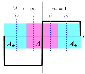
Figure 2: The four regions in the domain wall construction of Ref. Grabowska and Kaplan (2016).

IV.3 $\hat{\cal D}_{\chi}$ does not suffer from phase ambiguity

To see that there is no phase ambiguity in the definition of the determinant of $\hat{\cal D}_{\chi}$, it is convenient to consider the five-dimensional domain wall construction of Ref. Grabowska and Kaplan (2016) shown in Fig. 2, with a Dirac fermion living in the space $s\in[-L,L]$ with $s=\pm L$ identified. The fermion mass changes sign across the defects at $s=0$ and $s=\pm L$, while the gauge field equals $A$ near the $s=0$ defect and $A_{\star}$ near the $s=L$ defect. Two Pauli-Villars fields can be introduce to eliminate bulk effects, one with mass $M$ on $s\in[-L,0]$ and the other with mass $-m$ on $s\in[0,L]$, both with anti-periodic boundary conditions in $s$. Thus there are four distinct regions in $s$ corresponding to the two values for the fermion mass and the two values of the gauge field, described by the Hamiltonians

$$H_{1} = \gamma_{5}\left(D_{w}(A)+M\right)\ ,$$ (47)

$$H_{2} = \gamma_{5}\left(D_{w}(A)-m\right)\ ,$$ (48)

$$H_{3} = \gamma_{5}\left(D_{w}(A_{\star})-m\right)\ ,$$ (49)

$$H_{4} = \gamma_{5}\left(D_{w}(A_{\star})+M\right)\ ,$$ (50)

where $D_{w}$ is the Wilson operator given in Eq. (15), and we will take $M\to\infty$ and set $m=1$ in lattice units.

In the original Narayanan-Neuberger derivation, there is no gradient flow and so $A_{\star}=A$. Inserting a complete basis of states at two of the four s-slices (i and ii in Fig. 2) and taking the large $L$ limit, with the distances between all the relevant surfaces becoming infinite, all excited energy states are projected out and the partition function can be expressed in terms of the many-body ground states of the Hamiltonians $H_{n}$, denoted $\ket{\Omega_{n}}$, as

$$\det{\cal D}_{V}=\frac{\braket{\Omega_{1}}{\Omega_{2}}\braket{\Omega_{2}}{\Omega_{1}}}{\braket{\Omega_{1}}{\Omega_{1}}\braket{\Omega_{2}}{\Omega_{2}}}\ ,$$ (51)

where the numerator arises from the fermions while the denominator is due to the Pauli-Villars fields. The $\ket{\Omega_{n}}$ ground states in each case correspond to a filled Dirac sea and their overlap can be expressed as determinants of the overlap of negative energy single-particle wavefunctions.

Extending the Narayanan-Neuberger procedure to the more complicated system we are interested in with $A_{\star}\neq A$, we insert a complete set of states at all four $s$-slices (i-iv) shown in Fig. 2 and take the $L\to\infty$ limit. Again, the partition function can be expressed in terms of the $\ket{\Omega_{n}}$ states as

$$\det\hat{\cal D}_{\chi}=\frac{\braket{\Omega_{1}}{\Omega_{2}}\braket{\Omega_{2}}{\Omega_{3}}\braket{\Omega_{3}}{\Omega_{4}}\braket{\Omega_{4}}{\Omega_{1}}}{\left|\braket{\Omega_{2}}{\Omega_{3}}\right|^{2}\left|\braket{\Omega_{1}}{\Omega_{4}}\right|^{2}}\ .$$ (52)

While Eq. (52) is not particularly useful for deriving $\hat{\cal D}_{\chi}$, the cyclic arrangement of the four $\ket{\Omega_{n}}\bra{\Omega_{n}}$ factors in the numerator – which follows from the compact nature of the fifth dimension in the domain wall formulation – makes this expression for the chiral partition function both manifestly complex and independent of any phase convention for the ground states $\ket{\Omega_{n}}$. This is to be contrasted with earlier attempts to define the chiral determinant on a non-compact fifth dimension Kaplan (1992); Narayanan and Neuberger (1994) which suffered the same phase ambiguity encountered in defining the chiral fermion determinant in the four-dimensional continuum, namely that the right and left Hilbert spaces are subject to independent phase conventions.

V The Index of the chiral overlap operator

The $U(1)_{A}$ anomaly for the vector overlap operator can be expressed by the index theorem

$$-{\textstyle{\frac{1}{2}}}{\rm Tr\,}\gamma_{5}{\cal D}_{V}=-\nu=(N_{+}-N_{-})\ ,$$ (53)

where $N_{\pm}$ are the number of exact zeromodes of ${\cal D}_{V}$ and $\nu$ is defined in Eq. (37). Only the fact that ${\cal D}_{V}$ satisfies the GW equation is required to prove this relation Luscher (1998). In the continuum limit and for smooth gauge fields, the integer $\nu$ as calculated from $\epsilon$ can be equated to the usual topological winding number of the gauge fields, proportional to $\int{\rm Tr\,}F\widetilde{F}$. In this case Eq. (53) coincides with the continuum index theorem for a Dirac fermion Fujikawa (1999); Adams (2002); Suzuki (1999).

To understand what to expect for the index equation for ${\cal D}_{\chi}$ analogous to Eq. (53) we first consider the continuum operator Eq. (6). From the properties of the Dirac operator in a background gauge field $A$ with winding number $\nu$, we know that there are ${\textstyle{\frac{1}{2}}}(|\nu|+\nu)$ normalizable 2-component solutions to the differential equation

$$D_{\mu}(A)\sigma_{\mu}\phi=0\ ,$$ (54)

and ${\textstyle{\frac{1}{2}}}(|\nu|-\nu)$ normalizeable solutions to

$$(D_{\mu}(A))^{\dagger}\sigma_{\mu}\phi=0\ .$$ (55)

Here we are ignoring “accidental zeromode” solutions for special gauge field which are not mandated by topology. Analogous equations hold substituting $A\to A_{\star}$ and $\nu\to\nu_{\star}$. Since $\bar{\sigma}_{\mu}=\sigma_{\mu}^{\dagger}$ if follows that ${\cal D}_{\chi}$ in Eq. (6) has $n_{\pm}$ right zeromodes with chirality $\pm 1$ and $\bar{n}_{\pm}$ left zeromodes with chirality $\pm 1$ where

$$n_{+} =\frac{|\nu_{\star}|-\nu_{\star}}{2}\ ,\quad n_{-} =\frac{|\nu|+\nu}{2}\ ,$$ (56)

$$\bar{n}_{+} =\frac{|\nu|-\nu}{2}\ , \bar{n}_{-} =\frac{|\nu_{\star}|+\nu_{\star}}{2}\ .$$

giving rise to nonzero matrix elements of the generic form

$$\langle{\bar{\psi}}^{\bar{n}_{-}}_{R}{\bar{\psi}}^{\bar{n}_{+}}_{L}\psi^{n_{+}}_{R}\psi^{n_{-}}_{L}\rangle$$ (57)

which violates the chiral charge by

$$\Delta Q_{5} = -\left(\underbrace{(n_{-}-\bar{n}_{+})}_{\nu}+\underbrace{(\bar{n}_{-}-n_{+})}_{\nu_{\star}}\right)$$ (58)

$$= -(\nu+\nu_{\star})\ .$$

Thus we expect the analogue to Eq. (53) for the chiral operator should be

$$-{\rm Tr\,}\gamma_{5}{\cal D}_{\chi}=-(\nu+\nu_{\star})=2(N_{+}-N_{-})\ ,$$ (59)

where

$$n_{-}=\bar{n}_{-}=N_{-}\ ,\quad n_{+}=\bar{n}_{+}=N_{+}\ .$$ (60)

We now compute the lattice version of Eq. (59) directly from our expression for $\hat{\cal D}_{\chi}$, understood as the limit in Eq. (33). Since $\hat{\cal D}_{\chi}$ obeys the GW equation, it too obeys the chiral anomaly equation

$$-{\rm Tr\,}\gamma_{5}\hat{\cal D}_{\chi}=-{\rm Tr\,}\hat{\cal E}_{\chi}=2(N_{+}-N_{-})\ ,$$ (61)

with

$$\hat{\cal E}_{\chi}=\left[1-\left(1-\epsilon_{\star}\right)\frac{1}{1+\epsilon\,\epsilon_{\star}}\left(1-\epsilon\right)\right]\ .$$ (62)

What remains to do, then, is to show that ${\rm Tr\,}\hat{\cal E}_{\chi}=(\nu+\nu_{\star})$. This is easy to do for the case of topology preserving flow, where $\nu=\nu_{\star}$. As discussed in the appendix, for this case $(1+\epsilon\,\epsilon_{\star})$ is invertible and the trace can be trivially computed using the form in Eq. (46) with the desired result that

$${\rm Tr\,}\hat{\cal E}_{\chi}=2\nu\qquad\text{for}\,\nu=\nu_{\star}\ .$$ (63)

For unconstrained $\nu$ and $\nu_{\star}$, relevant for when the lattice gradient flow equation causes topology to vanish, the analysis is more complicated since $(1+\epsilon\,\epsilon_{\star})$ is no longer invertible and $\hat{\cal E}_{\chi}$ must be defined as the limit in Eq. (33). In Eq. (102) this trace is computed with the result

$${\rm Tr\,}\hat{\cal E}_{\chi}=(\nu+\nu_{\star})+\sum_{i=1}^{|\nu-\nu_{\star}|}\xi_{i}\ ,\qquad\xi_{i}=\pm 1\ .$$ (64)

In the above expression the first term is the contribution from eigenstates of $U=\epsilon\epsilon_{\star}$ with eigenvalue $+1$, and the second term is the contribution from eigenstates of $U$ with eigenvalue $-1$. This second term vanishes when the flow preserves topology and $\nu=\nu_{\star}$ . The $\xi_{i}$ parameters cannot be determined solely in terms of $\nu$ and $\nu_{\star}$ as they depend on the interplay between the two gauge fields; they must take on values of $\pm 1$. While $U$ also has eigenstates with generally complex eigenvalues, they are shown not to contribute to the trace. We see that for cases where $|\nu-\nu_{\star}|$ is an even integer it might be possible for the $\xi_{i}$ sum to vanish, recovering the correct continuum anomaly Eq. (59); however for odd $|\nu-\nu_{\star}|$ this is never possible.

The conclusion of this section is that when we assume a rapid transition from $A$ to $A_{\star}$ in the bulk, obtaining the correct index theorem requires topology preserving gradient flow on the lattice.

VI Problems with sudden flow

In order to be able to treat the derivation of the chiral overlap operator analytically we have chosen to consider the sudden flow scenario pictured in the third panel of Fig. 1, instead of the gradual flow shown in the middle panel. This allowed us to replace the general form for the product of transfer matrices in Eq. (27) with the more tractable form in Eq. (31). From the five-dimensional picture, however, the decoupling of fermions on one surface from their mirror partners on the other relied on the fermions having purely local interactions with a mass gap in the bulk. In effect the sudden transition from $A$ to $A_{\star}$ in the middle of the sample implies that a fermion in the bulk can couple simultaneously to the gauge fields at both boundaries. On integrating out the bulk fermion one can then in principle generate gauge invariant operators which are functions of the difference $(A-A_{\star})$, an object that transforms homogeneously under gauge transformations.

An example of such an unwanted term for the theory considered here in the sudden gauge field flow scenario was found in Ref. Makino and Morikawa (2016), which computed the anomaly for smooth gauge fields. The authors of that paper found that the divergence of the fermion current included a Lorentz-violating operator of the form

$$\sum_{\mu}\partial_{\mu}{\rm Tr\,}C^{3}_{\mu}\ ,$$ (65)

where $C=(A_{\star}-A)$. This result implies that $\nu$ and $\nu_{\star}$ are not given by the standard gauge field winding number in the continuum limit. This operator is seen to vanish under the same condition that ensures cancellation of gauge anomalies, namely that the symmetrized trace of three gauge generators vanishes, ${\rm Tr\,}T_{a}\{T_{b},T_{c}\}=0$. However, chiral gauge theories will contain other $U(1)$ charges for which such a term will not vanish. A simple example is an $SU(5)$ chiral gauge theory with Weyl fermions transforming as $\bar{5}\oplus 10$. Such a theory has no $SU(5)$ gauge anomaly; it also has an anomaly-free global $U(1)$ symmetry where the $\bar{5}$ carries charge $Q=3$ and the $10$ carries charge $Q=-1$. The results of Ref. Makino and Morikawa (2016) imply that computation of the divergence of this current on the lattice using the sudden flow result Eq. (36) will result in a term of the form

$$\sum_{\mu}\partial_{\mu}{\rm Tr\,}QC^{3}_{\mu}\$$ (66)

which will not vanish. This result, which persists in the continuum limit, is incompatible with the fermion determinant successfully factorizing into fermion and mirror contributions. From the five-dimensional picture we do not expect such terms to exist when gradual gauge flow is used, as in Eq. (27), but that remains to be shown.

VII Discussion

We have considered here the lattice formulation of the proposal in Ref. Grabowska and Kaplan (2016) for combining five-dimensional domain wall fermions with gradient flow for the gauge fields. Our proposal Eqs. (28-30) for a chiral fermion operator follows a venerable list of such proposals in the literature that have succumbed for various reasons. Therefore it is important to explore this new one further, both analytically and numerically, to test its viability. In particular it is important to understand better the issue of factorization of the fermion determinant in the continuum limit. One possibly interesting avenue for numerical exploration is the role of topologically induced interactions between matter and fluff, as discussed briefly in Ref. Grabowska and Kaplan (2016), and whether they persist in the large volume limit. These questions can most likely be explored by constructing $D_{\chi}$ for two fermions in conjugate representations of the gauge group, so that the “chiral” gauge theory being considered is actually vector-like. Choosing a theory such as QCD, which has been well-studied on the lattice, allows for comparison with conventionally obtained results and is likely to not be afflicted by a sign problem, unlike less trivial chiral gauge theories.

In order to treat $D_{\chi}$ explicitly we considered the particular choice of abrupt flow from $A$ to $A_{\star}$, pictured in the third panel of Fig. 1, for which the expression $\hat{D}_{\chi}$ was derived in Eq. (32). This allowed us to illustrate explicitly that $\hat{\cal D}_{\chi}$ obeyed the GW equation and, for topology preserving flow, gave the relation between the its index and the topological index $\nu$. However, in relating $\nu$ to the winding number of smooth gauge fields, the results of Ref. Makino and Morikawa (2016) exhibit a pathological dependence on the gauge fields which indicates that fermions and their mirrors do not successfully decouple from each other. We therefore believe that the gradual flow form given by Eq. (27) is the proper formulation of our idea, although we do not have a simple analytical form for the fermion operator in this case. Since our conclusion that the flow has to be topology preserving is only based on the abrupt flow scenario, we remain agnostic about whether or not a topology changing flow equation on the lattice must be ruled out entirely.

It is also necessary to better understand better the role of gauge anomalies, a topic not addressed in this paper. A feature of our proposal is that it is manifestly gauge invariant, while a chiral gauge theory with an anomalous fermion representation in the continuum is not. In the five-dimensional domain wall construction of the theory, models which do not have anomaly cancellation at each defect are characterized by a nonzero coefficient for a bulk Chern-Simons operator, which is nonlocal due to the gradient flow of the gauge field Grabowska and Kaplan (2016). We have not explored here the consequences of anomalous fermion representations for our four-dimensional chiral overlap operator $\hat{\cal D}_{\chi}$. The subject of global anomalies has also been recently explored for domain wall fermions with gradient flow in Ref. Fukaya et al. (2016), but how that physics manifests itself in the chiral overlap operator remains to be explored.

Finally, it would be gratifying to be able to establish a connection between the chiral overlap operator derived here, and Lüscher’s lattice construction of Abelian chiral gauge theories and consistency conditions on nonabelian ones presented in Refs. Luscher (2000, 1999).

Appendix A Properties of $\epsilon\epsilon_{\star}$

Here we discuss some properties of the matrix $U\equiv\epsilon\epsilon_{\star}$, where $\epsilon$ and $\epsilon_{\star}$ are the sign functions of two independent $2N\times 2N$ hermitian matrices $H$ and $H_{\star}$,

$$\epsilon=\frac{H}{\sqrt{H^{2}}}\ ,\qquad\epsilon_{\star}=\frac{H_{\star}}{\sqrt{H_{\star}^{2}}}\ ,$$ (67)

with traces given by

$${\rm Tr\,}\epsilon=2\nu\ ,\qquad{\rm Tr\,}\epsilon_{\star}=2\nu_{\star}\ .$$ (68)

The properties of

$$U\equiv\epsilon\epsilon_{\star}$$ (69)

are important for understanding our expression for $D_{\chi}$ as it involves the inverse of $\Delta^{+}=(1+U)$; these properties are examined in this section.

Lemma 1

Eigenvalues of $U$ take the values of $\pm 1$, or come in complex conjugate pairs, where $\epsilon$ is the conjugation matrix.

As matrix $U$ is unitary its eigenvalues are phases; left and right eigenvectors are conjugates of each other and we can represent them using Dirac’s bra-ket notation:

$$U\ket{m}=\eta_{m}\ket{m}\ ,\quad\bra{m}U=\eta_{m}\bra{m}\$$ (70)

with $|\eta_{m}|^{2}=$ and $\braket{m}{n}=\delta_{mn}$. The state $\ket{m}$ must also satisfy

$$U^{\dagger}\ket{m}=\eta_{m}^{*}\ket{m}\ .$$ (71)

Since $U=\epsilon\epsilon_{\star}$ and $U^{\dagger}=\epsilon_{\star}\epsilon$,

$$U\epsilon\ket{m}=\epsilon U^{\dagger}\ket{m}=\eta_{m}^{*}\epsilon\ket{m}\ .$$ (72)

Therefore the complex eigenvalues of $U$ must come in conjugate pairs, while the real eigenvalues can only take the values $+1$ or $-1$.

Lemma 2

The number of non-accidental $\pm 1$ eigenvalues of $U$ equals $|\nu\pm\nu_{\star}|$.

If we define the projection operators $Q^{\pm}$ and $Q_{\star}^{\pm}$ as

$$Q^{\pm}=\frac{1\pm\epsilon}{2}\ ,\quad Q_{\star}^{\pm}=\frac{1\pm\epsilon_{\star}}{2}\ ,$$ (73)

and

$$\Delta^{\pm}\equiv(1\pm U)\ .$$ (74)

then they are related by

$$\Delta^{+} = \epsilon(\epsilon+\epsilon_{\star})=2\epsilon\left(Q^{+}-Q^{-}_{\star}\right)=2\epsilon\left(Q^{+}_{\star}-Q^{-}\right)\ ,$$ (75)

$$\Delta^{-} = \epsilon(\epsilon-\epsilon_{\star})=2\epsilon\left(Q^{+}-Q^{+}_{\star}\right)=2\epsilon\left(Q^{-}_{\star}-Q^{-}\right)\ .$$ (76)

If these are all $2N\times 2N$ matrices, then $\epsilon$ is rank $2N$ while $Q^{\pm}$ and $Q^{\pm}_{\star}$ are rank $N\pm\nu$ and $N\pm\nu_{\star}$ respectively. It follows from the subadditivity of rank that

$$\text{rank}\,\Delta^{\pm}\leq 2N-|\nu\mp\nu_{\star}|\ ,$$ (77)

meaning that $\Delta^{\pm}$ must have at least $|\nu\mp\nu_{\star}|$ zero eigenvalues. We will assume that typically this inequality is saturated, and that additional accidental zeromodes are not important. Thus $U$ has $|\nu\pm\nu_{\star}|$ non-accidental eigenvalues equal to $\pm 1$ respectively. It immediately follows that $(1+U)$ is not invertible when $\nu\neq\nu_{\star}$.

Lemma 3

Eigenstates of $U$ corresponding to eigenvalues $\pm 1$ can be taken to be simultaneous eigenstates of $\epsilon$ and $\epsilon_{\star}$.

From Eq. (72), if $\ket{+1}$ satisfies $U\ket{+1}=\ket{+1}$, then so does the state $\epsilon\ket{+1}$. Therefore we can take as our basis vectors the nonvanishing $Q^{\pm}\ket{+1}$ vectors. These are eigenstates of $\epsilon$ with eigenvalues $\pm 1$ respectively. It follows from the definition $U=\epsilon\epsilon_{\star}$ that these states are also simultaneous eigenstates of $\epsilon_{\star}$ with eigenvalue $\pm 1$ respectively.

Similar reasoning for an eigenstate $\ket{-1}$ satisfying $U\ket{-1}=-\ket{-1}$ leads to states $Q^{\pm}\ket{-1}$ which are eigenstates of $\epsilon$ with eigenvalue $\pm 1$, and of $\epsilon_{\star}$ with eigenvalue $\mp 1$ respectively.

Lemma 4

The non-accidental eigenstates of $U$ with eigenvalue $\pm 1$ are simultaneous eigenstates of $\epsilon$ with eigenvalue ${\rm Sign}[\nu\pm\nu_{\star}]$

An index theorem for $U$ can be proven by adapting the methods of Luscher (1998). We note that $\Delta^{\pm}$ satisfy equations similar to the GW equation, with $\epsilon$ playing the role of $\gamma_{5}$:

$$\left\{\Delta^{\pm},\epsilon\,\right\}=\Delta^{\pm}\,\epsilon\,\Delta^{\pm}\ ,$$ (78)

from which one can derive the relation

$$(z-\Delta^{\pm})\epsilon\,(z-\Delta^{\pm})\hskip 140.92627pt\$$ (81)

$$\ =z(2-z)\epsilon-(1-z)\left[(z-\Delta^{\pm})\epsilon+\epsilon\,(z-\Delta^{\pm})\right]$$

for arbitrary complex variable $z$. Multiplying this on the right by $(z-\Delta^{\pm})^{-1}$ and taking the trace yields

$$-{\rm Tr\,}\epsilon\,\Delta^{\pm} = -(2-z){\rm Tr\,}\epsilon$$ (82)

$$+ z(2-z){\rm Tr\,}\epsilon\,(z-\Delta^{\pm})^{-1}\ .$$

Integrating this equation on a sufficiently small circle about the origin in the complex $z$ plane yields the index theorem. The integral

$$(\nu\mp\nu_{\star})={\rm Tr\,}\epsilon\,{\cal P}^{\pm}_{0}=(\mathfrak{n}^{\pm}_{+}-\mathfrak{n}^{\pm}_{-})\ ,$$ (83)

where

$${\cal P}^{\pm}_{0}=\oint\frac{dz}{2\pi i}(z-\Delta^{\pm})^{-1}$$ (84)

serves as a projector onto the space of zeromodes of $\Delta^{\pm}$. In Eq. (83), $\mathfrak{n}^{\pm}_{+}$ is the number of states in the kernel of $(1\pm U)$ that are simultaneously eigenstates of $\epsilon$ with eigenvalue $+1$, and $\mathfrak{n}^{\pm}_{-}$ is the number of states in the kernel of $(1\pm U)$ that are simultaneously eigenstates of $\epsilon$ with eigenvalue $-1$. Again assuming that there are no accidental zeromodes, we conclude that

$$\{\mathfrak{n}^{+}_{+},\mathfrak{n}^{+}_{-}\}=\begin{cases}\{|\nu-\nu_{\star}|,0\}&\nu>\nu_{\star}\\ \{0,0\}&\nu=\nu_{\star}\\ \{0,|\nu-\nu_{\star}|\}&\nu<\nu_{\star}\end{cases}\ ,$$ (85)

and

$$\{\mathfrak{n}^{-}_{+},\mathfrak{n}^{-}_{-}\}=\begin{cases}\{|\nu+\nu_{\star}|,0\}&\nu>-\nu_{\star}\\ \{0,0\}&\nu=-\nu_{\star}\\ \{0,|\nu+\nu_{\star}|\}&\nu<-\nu_{\star}\end{cases}\ .$$ (86)

Accidental zeromodes will occur when a pair of states with eigenvalues $e^{\pm i\delta}$ exhibits a level crossing with $\delta$ passing through a multiple of $\pi$. For the particular gauge field for which such a crossing occurs, both $\mathfrak{n}^{-}_{\pm}$ will change by one if at $\delta=0\ \text{Mod}[2\pi]$, while both $\mathfrak{n}^{+}_{\pm}$ will change by one if at $\delta=\pi\ \text{Mod}[2\pi]$.

Appendix B Matrix elements of $\hat{\cal E}_{\chi}$ for general gauge field topology

Our proposal for $\hat{\cal D}_{\chi}$ in Eq. (36) is

$$\hat{\cal D}_{\chi} = 1+\gamma_{5}\hat{\cal E}_{\chi}\ ,$$ (87)

$$\hat{\cal E}_{\chi} = 1-(1-\epsilon_{\star})\frac{1}{1+U}(1-\epsilon)\ .$$ (88)

where $U=\epsilon\epsilon_{\star}$ as in Eq. (69). In Sec. IV.2 we showed that $\hat{\cal D}_{\chi}$ obeyed the GW equation whenever the matrix $\Delta^{+}=(1+U)$ is invertible. This only occurs when $\nu=\nu_{\star}$, as was shown in the previous appendix, Lemma 2. Using the definition of these quantities in Eq. (68), we conclude that $1+U$ is only invertible when the gradient flow preserves topology. In order to show that $\hat{\cal D}_{\chi}$ generally obeys the GW equation for any type of gauge-covariant flow equation, one must generalize $\hat{\cal E}_{\chi}$ to the case when $\Delta^{+}=(1+U)$ is not invertible, which we do here. This will also allow us to compute ${\rm Tr\,}\hat{\cal E}_{\chi}$, which is the chiral index of $\hat{\cal D}_{\chi}$ and yields the chiral anomaly.

To better understand $\hat{\cal E}_{\chi}$ when $\nu\neq\nu_{\star}$ we can use eigenstates of $U$ to define the Hilbert space, which is divided into three distinct subspaces spanned by states $\ket{I}$, $\ket{m}$, $\ket{i}$ where

$$U\ket{I} = \ket{I}\ ,\ I =1,\ldots,|\nu+\nu_{\star}|$$ (89)

$$U\ket{i} = -\ket{i}\ ,\ i =1,\ldots,|\nu-\nu_{\star}|$$

$$U\ket{m} = \eta_{m}\ket{m}\ ,\ m =1,\ldots,2N-|\nu+\nu_{\star}|-|\nu-\nu_{\star}|\ ,$$

with $|\eta_{m}|=1$ and $\eta_{m}\neq\pm 1$; the complex eigenvalues come in complex conjugate pairs. The action of $\epsilon$ and $\epsilon_{\star}$ on these states is

$$\epsilon\ket{I} = +\epsilon_{\star}\ket{I} = \text{ sign}[\nu+\nu_{\star}]\ket{I}$$ (90)

$$\epsilon\ket{i} = -\epsilon_{\star}\ket{i} = \text{ sign}[\nu-\nu_{\star}]\ket{i}\ ,$$

while

$$\epsilon\ket{m}\equiv\ket{\kern 0.6pt\overline{\kern-0.6ptm\kern-0.6pt}\kern 0.6pt}\ ,\quad\epsilon_{\star}\ket{m}\equiv\eta_{m}\ket{\kern 0.6pt\overline{\kern-0.6ptm\kern-0.6pt}\kern 0.6pt}$$ (91)

where $\ket{\kern 0.6pt\overline{\kern-0.6ptm\kern-0.6pt}\kern 0.6pt}$ is the state with $U$ eigenvalue $\eta_{m}^{*}$, and we have made a particular phase choice in its definition.

It is evident that in this basis the matrix $\hat{\cal E}_{\chi}$ is diagonal in the $\ket{I}$, $\ket{i}$ sectors, and is block diagonal in the remaining space, in $2\times 2$ blocks acting on each $\left\{\ket{m},\ket{\bar{m}}\right\}$ pair of states. Using the results in the above equations, the nonzero matrix elements of $\hat{\cal E}_{\chi}$ are given by

$$\langle I|\hat{\cal E}_{\chi}|I\rangle = \text{ sign}[\nu+\nu_{\star}]\ ,$$ (92)

$$\langle i|\hat{\cal E}_{\chi}|i\rangle = \xi_{i}\ ,$$ (94)

$$\begin{pmatrix}\bra{m}\\ \bra{\kern 0.6pt\overline{\kern-0.6ptm\kern-0.6pt}\kern 0.6pt}\end{pmatrix}\,\hat{\cal E}_{\chi}\,\begin{pmatrix}\ket{m}&\ket{\kern 0.6pt\overline{\kern-0.6ptm\kern-0.6pt}\kern 0.6pt}\end{pmatrix} = \frac{1}{1+\eta_{m}}\begin{pmatrix}\eta_{m}-1&2\\ 2\eta_{m}&1-\eta_{m}\end{pmatrix}$$ (97)

$$\ .$$

In order for $\hat{\cal D}_{\chi}$ to satisfy the GW equation, $\hat{\cal E}_{\chi}^{2}=1$ and, given that

$$\left(\text{ sign}[\nu+\nu_{\star}]\right)^{2} = 1\ ,$$ (98)

$$\frac{1}{(1+\eta_{m})^{2}}\begin{pmatrix}\eta_{m}-1&2\\ 2\eta_{m}&1-\eta_{m}\end{pmatrix}^{2} = \begin{pmatrix}1&0\\ 0&1\end{pmatrix}\ ,$$ (100)

it follows that $\xi_{i}^{2}=1$ for every index $i$.

If we naively try to compute the $\xi_{i}=\langle i|\hat{\cal E}_{\chi}|i\rangle$ matrix elements from Eq. (89) and Eq. (90) we will find the ratio of two vanishing quantities. Nevertheless, as was shown in Sec. IV the eigenvalues of $\hat{\cal E}_{\chi}$ are bounded between $\pm 1$, and as the $\xi_{i}$ are such eigenvalues, it follows that

$$-1\leq\xi_{i}\leq 1\ .$$ (101)

Furthermore, we argued that except at exceptional gauge fields that relate the spectrum of $H$ to that of $H_{\star}$ in a special way, the $\xi_{i}$ must saturate the bounds with $\xi_{i}=\pm 1$.

What this argument does not tell us is how many of the $\xi_{i}$ equal $+1$ and how many equal $-1$; it is not possible to determine this knowing $\nu$ and $\nu_{\star}$ alone. To see this, consider rescaling $H$ and $H_{\star}$ by number $c$ and $c_{\star}$ respectively. These rescalings do not affect $\epsilon$ or $\epsilon_{\star}$. If $c\to 0$ while $c_{\star}=1$ then we can ignore $T$ in Eq. (33) and $\hat{\cal E}_{\chi}\to\epsilon$; if we do the reverse, then we get $\hat{\cal E}_{\chi}\to\epsilon_{\star}$. Thus by changing $H$ and $H_{\star}$ relative to each other without changing the signs of their eigenvalues, we can change the trace of $\hat{\cal E}_{\chi}$, presumably by jumps of 2 as successive $\xi_{i}$ change sign.

We conclude that, except for exceptional gauge fields, $\hat{\cal E}_{\chi}$ obeys the GW equation, and that it is precisely when one passes through those special gauge fields that it is possible for the trace of $\hat{\cal E}_{\chi}$ to jump by $\pm 2$.

For the anomaly we need to compute the trace of $\hat{\cal E}_{\chi}$. Using the above analysis, we find

$${\rm Tr\,}\hat{\cal E}_{\chi}=(\nu+\nu_{\star})+\sum_{i=1}^{|\nu-\nu_{\star}|}\xi_{i}$$ (102)

where the first term comes from the $\ket{I}$ space where $\epsilon\epsilon_{*}=+1$, and the second term arises from the $\ket{i}$ space where $\epsilon\epsilon_{*}=-1$. Note that the complex eigenvalue sectors do not contribute as the corresponding $2\times 2$ matrix elements in Eq. (97) are traceless.

References

- Alvarez-Gaume and Ginsparg (1984) L. Alvarez-Gaume and P. H. Ginsparg, Nucl. Phys. B243, 449 (1984).
- Alvarez-Gaume et al. (1986) L. Alvarez-Gaume, S. Della Pietra, and V. Della Pietra, Phys. Lett. B166, 177 (1986).
- Fujikawa (1979) K. Fujikawa, Phys. Rev. Lett. 42, 1195 (1979).
- Adler (1969) S. L. Adler, Phys. Rev. 177, 2426 (1969).
- Bell and Jackiw (1969) J. S. Bell and R. Jackiw, Nuovo Cimento A Serie 60, 47 (1969).
- Ginsparg and Wilson (1982) P. H. Ginsparg and K. G. Wilson, Phys. Rev. D25, 2649 (1982).
- Hasenfratz et al. (1998) P. Hasenfratz, V. Laliena, and F. Niedermayer, Phys. Lett. B427, 125 (1998), arXiv:hep-lat/9801021 [hep-lat] .
- Luscher (1998) M. Luscher, Phys. Lett. B428, 342 (1998), arXiv:hep-lat/9802011 [hep-lat] .
- Narayanan and Neuberger (1994) R. Narayanan and H. Neuberger, Nucl. Phys. B412, 574 (1994), arXiv:hep-lat/9307006 [hep-lat] .
- Narayanan and Neuberger (1995) R. Narayanan and H. Neuberger, Nucl. Phys. B443, 305 (1995), arXiv:hep-th/9411108 [hep-th] .
- Neuberger (1998a) H. Neuberger, Phys.Lett. B417, 141 (1998a), arXiv:hep-lat/9707022 [hep-lat] .
- Neuberger (1998b) H. Neuberger, Phys. Lett. B427, 353 (1998b), arXiv:hep-lat/9801031 [hep-lat] .
- Golterman and Shamir (2004) M. Golterman and Y. Shamir, Physical Review D 70, 094506 (2004).
- Golterman (2001) M. Golterman, Nucl. Phys. Proc. Suppl. 94, 189 (2001), arXiv:hep-lat/0011027 [hep-lat] .
- Luscher (2002) M. Luscher, Theory and experiment heading for new physics. Proceedings, 38th course of the International School of subnuclear physics, Erice, Italy, August 27-September 5, 2000, Subnucl. Ser. 38, 41 (2002), arXiv:hep-th/0102028 [hep-th] .
- Wen (2013) X.-G. Wen, Chin. Phys. Lett. 30, 111101 (2013), arXiv:1305.1045 [hep-lat] .
- Giedt et al. (2014) J. Giedt, C. Chen, and E. Poppitz, Proceedings, 31st International Symposium on Lattice Field Theory (Lattice 2013), PoS LATTICE2013, 131 (2014), arXiv:1403.5146 [hep-lat] .
- You and Xu (2015) Y.-Z. You and C. Xu, Physical Review B 91, 125147 (2015).
- Grabowska and Kaplan (2016) D. M. Grabowska and D. B. Kaplan, Phys. Rev. Lett. 116, 211602 (2016), arXiv:1511.03649 [hep-lat] .
- (20) D. M. Grabowska, Talk delivered at Lattice 2016: https://conference.ippp.dur.ac.uk/event/470/session/16/contribution/364 .
- (21) D. B. Kaplan, Talk delivered at Lattice 2016: https://conference.ippp.dur.ac.uk/event/470/session/1/contribution/398 .
- Kaplan (1992) D. B. Kaplan, Phys. Lett. B288, 342 (1992), arXiv:hep-lat/9206013 [hep-lat] .
- Kaplan (2009) D. B. Kaplan, in Modern perspectives in lattice QCD: Quantum field theory and high performance computing. Proceedings, International School, 93rd Session, Les Houches, France, August 3-28, 2009 (2009) pp. 223–272, arXiv:0912.2560 [hep-lat] .
- Callan and Harvey (1985) C. G. Callan, Jr. and J. A. Harvey, Nucl. Phys. B250, 427 (1985).
- Golterman et al. (1993) M. F. L. Golterman, K. Jansen, and D. B. Kaplan, Phys. Lett. B301, 219 (1993), arXiv:hep-lat/9209003 [hep-lat] .
- Jansen and Schmaltz (1992) K. Jansen and M. Schmaltz, Phys. Lett. B296, 374 (1992), arXiv:hep-lat/9209002 [hep-lat] .
- Shamir (1993) Y. Shamir, Nucl. Phys. B406, 90 (1993), arXiv:hep-lat/9303005 [hep-lat] .
- Furman and Shamir (1995) V. Furman and Y. Shamir, Nucl. Phys. B439, 54 (1995), arXiv:hep-lat/9405004 [hep-lat] .
- Jansen (1992) K. Jansen, Phys. Lett. B288, 348 (1992), arXiv:hep-lat/9206014 [hep-lat] .
- Kaplan (1993) D. B. Kaplan, Nucl. Phys. Proc. Suppl. 30, 597 (1993).
- Neuberger (1998c) H. Neuberger, Phys. Rev. D57, 5417 (1998c), arXiv:hep-lat/9710089 [hep-lat] .
- Kaplan and Schmaltz (2000) D. B. Kaplan and M. Schmaltz, Chiral gauge theories. Proceedings, Workshop, Chiral’99, Taipei, Taiwan, September 13-18, 1999, Chin. J. Phys. 38, 543 (2000), arXiv:hep-lat/0002030 [hep-lat] .
- Kane and Mele (2005) C. L. Kane and E. J. Mele, Phys. Rev. Lett. 95, 226801 (2005).
- Kitaev (2001) A. Y. Kitaev, Physics-Uspekhi 44, 131 (2001).
- Atiyah and Bott (1983) M. F. Atiyah and R. Bott, Philosophical Transactions of the Royal Society of London A: Mathematical, Physical and Engineering Sciences 308, 523 (1983).
- Narayanan and Neuberger (2006) R. Narayanan and H. Neuberger, JHEP 03, 064 (2006), arXiv:hep-th/0601210 [hep-th] .
- Luscher (2010) M. Luscher, JHEP 1008, 071 (2010), arXiv:1006.4518 [hep-lat] .
- Okumura and Suzuki (2016) K.-i. Okumura and H. Suzuki, (2016), arXiv:1608.02217 [hep-lat] .
- Luscher (1982) M. Luscher, Comm. Math. Phys. 85, 39 (1982).
- Teper (1985) M. Teper, Phys. Lett. B162, 357 (1985).
- Teper (1986a) M. Teper, Phys. Lett. B171, 81 (1986a).
- Teper (1986b) M. Teper, Phys. Lett. B171, 86 (1986b).
- Braam and van Baal (1989) P. J. Braam and P. van Baal, Commun. Math. Phys. 122, 267 (1989).
- Garcia Perez et al. (1990) M. Garcia Perez, A. Gonzalez-Arroyo, and B. Soderberg, Phys. Lett. B235, 117 (1990).
- de Forcrand et al. (1997) P. de Forcrand, M. Garcia Perez, and I.-O. Stamatescu, Nucl. Phys. B499, 409 (1997), arXiv:hep-lat/9701012 [hep-lat] .
- Garcia Perez et al. (1994) M. Garcia Perez, A. Gonzalez-Arroyo, J. R. Snippe, and P. van Baal, Nucl. Phys. B413, 535 (1994), arXiv:hep-lat/9309009 [hep-lat] .
- Vranas (1998) P. M. Vranas, Phys. Rev. D57, 1415 (1998), arXiv:hep-lat/9705023 [hep-lat] .
- Kikukawa and Noguchi (2000) Y. Kikukawa and T. Noguchi, Lattice field theory. Proceedings, 17th International Symposium, Lattice’99, Pisa, Italy, June 29-July 3, 1999, Nucl. Phys. Proc. Suppl. 83, 630 (2000), arXiv:hep-lat/9902022 [hep-lat] .
- Fujikawa (1999) K. Fujikawa, Nucl. Phys. B546, 480 (1999), arXiv:hep-th/9811235 [hep-th] .
- Adams (2002) D. H. Adams, Annals Phys. 296, 131 (2002), arXiv:hep-lat/9812003 [hep-lat] .
- Suzuki (1999) H. Suzuki, Prog. Theor. Phys. 102, 141 (1999), arXiv:hep-th/9812019 [hep-th] .
- Makino and Morikawa (2016) H. Makino and O. Morikawa, (2016), arXiv:1609.08376 [hep-lat] .
- Fukaya et al. (2016) H. Fukaya, T. Onogi, S. Yamamoto, and R. Yamamura, (2016), arXiv:1607.06174 [hep-th] .
- Luscher (2000) M. Luscher, Nucl. Phys. B568, 162 (2000), arXiv:hep-lat/9904009 [hep-lat] .
- Luscher (1999) M. Luscher, Nucl. Phys. B549, 295 (1999), arXiv:hep-lat/9811032 [hep-lat] .