Feasibility study for the measurement of $\pi N$ TDAs at $\overline{\mbox{\sf\bf P}}$ANDA in $\bar{p}p\to J/\psi\pi^{0}$

Abstract

The exclusive charmonium production process in $\bar{p}p$ annihilation with an associated $\pi^{0}$ meson $\bar{p}p\to J/\psi\pi^{0}$ is studied in the framework of QCD collinear factorization. The feasibility of measuring this reaction through the $J/\psi\to e^{+}e^{-}$ decay channel with the $\overline{\mbox{\sf P}}$ANDA (AntiProton ANnihilation at DArmstadt) experiment is investigated. Simulations on signal reconstruction efficiency as well as the background rejection from various sources including the $\bar{p}p\to\pi^{+}\pi^{-}\pi^{0}$ and $\bar{p}p\to J/\psi\pi^{0}\pi^{0}$ reactions are performed with PandaRoot, the simulation and analysis software framework of the $\overline{\mbox{\sf P}}$ANDA experiment. It is shown that the measurement can be done at $\overline{\mbox{\sf P}}$ANDA with significant constraining power under the assumption of an integrated luminosity attainable in four to five months of data taking at the maximum design luminosity.

I Introduction

Understanding of the hadronic structure in terms of the fundamental degrees of freedom of QCD is one of the fascinating questions of the present day physics. Lepton beam initiated reactions, allowing to resolve individual quarks and gluons inside hadrons, proved to be a handy tool for this issue. The factorization property established for several classes of hard (semi-)inclusive and exclusive processes allows to separate the short distance dominated stage of interaction and the universal non-perturbative hadronic matrix elements. Some of the matrix elements which have been the subject of significant interest include the Parton Distribution Functions (PDFs) Collins et al. (1989), Generalized Parton Distributions (GPDs) Guidal et al. (2013); Mueller (2014), Transverse Momentum Dependent Parton Distribution Functions (TMD PDFs) Barone et al. (2010), (Generalized) Distribution Amplitudes ((G)DAs) Braun et al. (1999) and Transition Distribution Amplitudes (TDAs) Frankfurt et al. (1999); Pire and Szymanowski (2005) encoding valuable information on the hadron constituents.

Alongside with the study of lepton beam induced reactions, one can get access to the same non-perturbative functions in a complementary way by considering the cross conjugated channels of the corresponding reactions. For example, proton-antiproton annihilation into a lepton pair and a photon (or a meson) can be seen as the cross conjugated counterpart of the leptoproduction of photons (or mesons) off protons, and provides access to nucleon GPDs and/or nucleon-to-photon (nucleon-to-meson) TDAs.

Such investigations have been hindered up to now by the limitations of antiproton beam luminosities. However, very significant results on the electromagnetic form factors in the time-like region using the $p\bar{p}\to e^{+}e^{-}$ reaction were obtained by the E835 experiment at FNAL (Fermilab National Accelerator Laboratory) Andreotti et al. (2003). But inclusive lepton pair production and hard exclusive channels still remain unexplored.

This situation will be largely improved in the next decade with the availability of the high intensity antiproton beam at FAIR (Facility for Antiproton and Ion Research) with momentum up to $15$ GeV/$c$. The $\overline{\mbox{\sf P}}$ANDA experiment Erni et al. (2009) will dedicate an important part of its physics program to the investigation of the nucleon structure in antiproton-proton annihilation reactions. It includes the detailed study of the time-like electromagnetic nucleon form factors employing both the $e^{+}e^{-}$ and $\mu^{+}\mu^{-}$ production channels in a broad kinematic range. It is also planned to access PDFs through the Drell-Yan mechanism, by measuring inclusive $e^{+}e^{-}$ production and GPDs considering $\gamma^{*}\gamma$ and $\gamma^{*}\pi^{0}$ exclusive channels at large production angles. Finally, the reactions $\bar{p}p\to\gamma^{*}M\to e^{+}e^{-}M$ and $\bar{p}p\to J/\psi M\to e^{+}e^{-}M$, where $M$ stands for a light meson $M=\{\pi^{0},\,\eta,\rho^{0},\,\omega,\,\ldots\}$, are proposed to study nucleon-to-meson TDAs.

Nucleon-to-meson (and particularly nucleon-to-pion) TDAs were introduced as a further generalization of the concepts of both GPDs and nucleon light-cone wave functions (DAs). They describe partonic correlations inside nucleons and allow to access the non-minimal Fock components of the nucleon light-cone wave function with additional quark-antiquark pair seen as a light meson. Therefore, in particular, $\pi N$ TDAs provide information on the nucleon’s pion cloud.

Nucleon-to-pion TDAs arise in the collinear factorized description of several hard exclusive reactions such as backward electroproduction of pions off nucleons Lansberg et al. (2007a, 2012a), which can be studied at JLab Kubarovskiy (2013) and COMPASS in the space-like regime, while $\overline{\mbox{\sf P}}$ANDA will provide access to the same non-perturbative functions in the time-like regime Lansberg et al. (2007b, 2012b).

On the theory side, the possibility to study nucleon-to-meson TDAs is provided by the collinear factorization theorem similar to the well known collinear factorization theorem for hard meson electroproduction Collins et al. (1997), giving rise to the description in terms of GPDs. However, the collinear factorization theorem for the TDA case has never been proven explicitly. Therefore, one of the important experimental tasks is to look for experimental evidence of the validity of the factorized description of the corresponding reactions in terms of nucleon-to-meson TDAs. This can be done either by verifying the appropriate scaling behavior or by checking the angular dependence of the produced lepton pair specific for the dominant reaction mechanism. Bringing trustworthy evidence for the validity of the factorized description of a new class of hard exclusive reaction will, by itself, represent a major experimental achievement of $\overline{\mbox{\sf P}}$ANDA.

Recently, a detailed study of the access to $\pi N$ TDAs in the reaction $\bar{p}p\to\gamma^{*}\pi^{0}\to e^{+}e^{-}\pi^{0}$ following the cross section estimates of Ref. Lansberg et al. (2007b) with $\overline{\mbox{\sf P}}$ANDA has been presented in Ref. Singh et al. (2015). The investigation of the reaction $\bar{p}p\to J/\psi\pi^{0}\to e^{+}e^{-}\pi^{0}$ constitutes a natural complement to the latter study. The resonant case presents the noticeable advantage of a larger cross section, and a cleaner signal selection due to the resonant $e^{+}e^{-}$ production. The simultaneous measurement of both resonant and non-resonant channels provides constraints to the $\pi N$ TDAs in different kinematic ranges, and allows to test the universality of $\pi N$ TDAs. While the non-resonant $\bar{p}p\to\gamma^{*}\pi^{0}\to e^{+}e^{-}\pi^{0}$ has never been measured, some scarce data exist for $\bar{p}p\to J/\psi\pi^{0}\to e^{+}e^{-}\pi^{0}$ Armstrong et al. (1992); Joffe (2004); Andreotti et al. (2005), which can be used to constrain the predictions. Production of a $J/\psi$ with an associated $\pi^{0}$ in $\bar{p}p$ collisions has indeed been investigated in the past by the E760 experiment at FNAL, since it constitutes a background in the search for charmonium states via their decay into $J/\psi\pi^{0}$. An important part of the $\overline{\mbox{\sf P}}$ANDA program will also focus on such studies, as described in Ref. Lundborg et al. (2006). This brings additional motivation for the detailed measurements of the $\bar{p}p\to J/\psi\pi^{0}\to e^{+}e^{-}\pi^{0}$ reaction. From the theory point of view, access to the $\pi N$ TDA in the $J/\psi$ production channel is also more favorable, since one can take advantage of the known $J/\psi\to\bar{p}p$ decay width Olive et al. (2014) in order to reduce ambiguities related to the choice of the phenomenological parametrization for the relevant nucleon DA Pire et al. (2013).

The aim of the present study is therefore to explore the feasibility of the measurement of the reaction $\bar{p}p\to J/\psi\pi^{0}\to e^{+}e^{-}\pi^{0}$ with $\overline{\mbox{\sf P}}$ANDA at different incident momenta of the antiproton beam, based on the cross section estimates of Ref. Pire et al. (2013). The paper is organized as follows: Section II outlines the design of the $\overline{\mbox{\sf P}}$ANDA experimental setup with a focus on the most relevant components to the analysis. Section III covers the properties of the $\bar{p}p\to J/\psi\pi^{0}\to e^{+}e^{-}\pi^{0}$ reaction which constitutes the signal. In Section IV, the different background contributions are discussed. Section V is devoted to the description of the simulation and analysis procedure. In Section VI, the expected precision on differential cross section measurements is presented.

II $\overline{\mbox{\sf\bf P}}$ANDA Experimental Setup

II.1 FAIR Accelerator Complex

The FAIR accelerator complex which is under construction to extend the existing GSI (Gesellschaft für Schwerionenforschung) facilities in Darmstadt, Germany, will provide beam for four experimental pillars, one of which is the $\overline{\mbox{\sf P}}$ANDA experiment dedicated to hadronic physics. FAIR will use the existing SIS18 synchrotron as an injection ring into a new larger synchrotron SIS100. The SIS100 ring will generate an intense pulsed beam of protons with energies reaching up to 29 GeV that can be directed at an antiproton production target. Time averaged production rates in the range of $5.6\times 10^{6}$ to $10^{7}~{}\bar{p}~{}s^{-1}$ are expected. Antiprotons are collected and phase space cooled in the CR (Collector Ring), then transferred to the RESR (Recycled Experimental Storage Ring) accumulator, and then injected into the HESR (High Energy Storage Ring), equipped with stochastic and electron cooling, where they will be used by the $\overline{\mbox{\sf P}}$ANDA experiment in a fixed target setup. This full setup is designed to provide beams with up to $10^{11}$ antiprotons, and peak instantaneous luminosities reaching up to $2\times 10^{32}$ cm^-2s^-1. Such a scenario will allow the accumulation of an integrated luminosity of 2 fb^-1 in about five months, which will be used as the basis for all results shown in this analysis. However, the more likely scenario currently is a staged construction with a reduced setup at the start of operations without the RESR until the full design can be realized. In this case, the HESR will be used as an accumulator in addition to its original task of cooling the beam and storing it for experiments with internal targets. This will result in a luminosity that is about a factor ten lower than the full design goal during the initial phases of operating FAIR.

II.2 The $\overline{\mbox{\sf\bf P}}$ANDA Detector

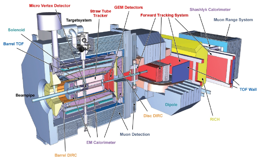
Figure 1: The proposed $\overline{\mbox{\sf P}}$ANDA experimental setup Erni et al. (2009).

The proposed $\overline{\mbox{\sf P}}$ANDA detector is depicted in Fig. 1. The discussion here will focus on the subsystems that are particularly relevant for the presented analysis. The $\overline{\mbox{\sf P}}$ANDA detector consists of the target spectrometer surrounding the target area and the forward spectrometer designed to detect particles in the forward rapidity region. The target spectrometer is divided into a barrel region with polar angle reach from 22^∘ to 145^∘, and an endcap region that covers polar angles below 22^∘, down to 10^∘ in the horizontal plane and 5^∘ in the vertical plane. Particles with polar angles below the endcap coverage are detected by the forward spectrometer. In addition, $\overline{\mbox{\sf P}}$ANDA will be equipped with a Luminosity Monitor Detector (LMD) at very forward angles, built for precise determination of both absolute and relative time integrated luminosities.

Two technologies are being developed to provide a hydrogen target with sufficient density that allows to reach the design luminosity within the restricted space available Erni et al. (2009). A target thickness of $4\times 10^{15}$ hydrogen atoms per cm² is required to achieve a peak luminosity of $2\times 10^{32}$ cm^-2s^-1 assuming 10¹¹ stored antiprotons in the HESR. The Cluster-Jet Target system operates by pumping pressurized cold hydrogen gas into vacuum through a Laval-type nozzle, leading to a condensation of hydrogen molecules into a narrow jet of hydrogen clusters with each cluster containing $10^{3}$ – $10^{6}$ hydrogen molecules. The main advantages of this setup are the homogeneous density profile and the ability to focus the antiproton beam at the highest areal density point. The Pellet Target system creates a stream of frozen hydrogen micro-spheres (pellets) of diameter 25 – 40 $\mathrm{\mu}$m, that cross the antiproton beam perpendicularly. The Pellet Target will be equipped with an optical tracking system that can determine the vertex position of individual events with high precision.

The innermost part of the barrel region is occupied by charged particle tracking detectors, which in turn are surrounded by particle identification detectors, followed by a solenoid magnet that generates a nearly uniform 2 T field pointing in the direction of the beam. The innermost layers of tracking are provided by the Micro Vertex Detector (MVD) Erni et al. (2012a), based on silicon pixel detectors for the innermost two layers, and a double sided strip detectors for the remaining two layers. The Straw Tube Tracker (STT) Erni et al. (2012b) is constructed from aluminized mylar tubes with gold-plated tungsten anode wires running along the axis. The tubes operate with an active gas mixture composed of argon and CO₂ held at a pressure of 2 bar allowing them to be mechanically self-supporting. The STT adds only about X/X${}_{0}\approx~{}1.2\%$ to the total radiation length of the tracking system on top of the $\approx~{}10\%$ expected from the MVD. The MVD and the STT also measure ionization energy loss by charged particles in their layers. A truncated mean of the specific energy loss of the tracks measured by the MVD and STT layers is used to estimate the energy loss $dE/dx$ for each track.

The barrel region tracking subsystems are immediately surrounded by various dedicated particle identification (PID) detectors. The innermost PID detector that is used in this analysis is the barrel DIRC Hoek et al. (2014) (Detection of Internally Reflected Cherenkov light), where particles are identified by the size of the Cherenkov opening angle. The DIRC is followed by the barrel Electromagnetic Calorimeter (EMC) Erni et al. (2008), constructed from lead tungstate (PbWO₄) doped crystals, operated at a temperature of -25^∘C to optimize the light yield. Photons from each crystal in the barrel EMC are detected by a pair of APDs (Avalanche Photodiodes). The EMC constitutes the most powerful detector for the identification of electrons through the momentum-energy correlation, particularly at momenta higher than $\approx$ 1 GeV/$c$. The DIRC, together with the MVD and STT $dE/dx$ measurements, ensure coverage at lower momenta where the EMC electron identification (EID) capacity is weaker.

The design of the barrel spectrometer of $\overline{\mbox{\sf P}}$ANDA also includes a Muon Range System (MRS) surrounding the Solenoid for the identification of muons as well as Time of Flight (TOF) detectors between the tracking layers and the DIRC for general PID. The MRS and TOF are not used in the analysis presented here.

For the endcap section of the target spectrometer, tracking points are provided by the STT as well as a set of four disc shaped MVD layers, and three chambers of Gas Electron Multiplier (GEM) trackers. PID is performed using information from the endcap EMC and the endcap DIRC Merle et al. (2014) (also called Disc DIRC in reference to its geometrical shape). Apart from its location, and angular coverage, the Disc DIRC operates using the same basic principle as the barrel DIRC. The endcap EMC is instrumented using the same PbWO₄ crystals as the barrel EMC, however photon detection is performed using APDs only for the outer lying crystals. The crystals close to the beam axis are readout by VPTs (Vacuum Phototriodes) because of the stringent requirements on radiation hardness there.

The design of $\overline{\mbox{\sf P}}$ANDA also provides for coverage at angles below those of the target spectrometer ($<5^{\circ}$), through the Forward Tracking System (FTS), a Ring Imaging Cerenkov (RICH) detector system and a Shashlyk calorimeter. Charged particles traversing the forward tracking system are subject to a field integral of 2 Tm generated by a dipole magnet, allowing for momentum determination. For this analysis, the forward Shashlyk calorimeter was not included in the simulations. As a result, our efficiency prediction is underestimated for events whose kinematics leads to charged particles requiring energy measurement for identification in the extremely forward direction. With the full $\overline{\mbox{\sf P}}$ANDA setup, the performance for such events will be better than that reported in this paper.

Precise determination of integrated luminosity is a critically important ingredient for the whole $\overline{\mbox{\sf P}}$ANDA physics program. The LMD is a detector that has been designed to provide both absolute and relative time integrated luminosity measurements with 5% and 1% systematic uncertainty, respectively Pan . The LMD will rely on the determination of the differential cross section of antiproton – proton elastic scattering into a polar angle (laboratory reference frame) range of 3.5 – 8 mrad and full azimuth to achieve this goal. The LMD tracks antiprotons using four planes of HV-MAPS (High Voltage Monolithic Active Pixel Sensors) tracking stations, a setup chosen to fulfil the constraints of high spatial resolution and low material budget. The LMD will be placed 10.5 m downstream from the interaction point within a vacuum sealed enclosure to reduce systematic uncertainties from multiple scattering.

II.3 Simulation and Analysis Software Environment

The simulation and analysis software framework called PandaRoot Bertini et al. (2008); Spataro (2012) is used for the feasibility study described here. PandaRoot is a collection of tools used for the simulation of the transport of particles through a GEANT4 Agostinelli et al. (2003) implementation of the $\overline{\mbox{\sf P}}$ANDA detector geometry, as well as detailed response simulation and digitization of hits in the various detector elements that takes into account electronic noise. Software for the reconstruction of tracks based on the simulated tracking detector hit points is implemented in PandaRoot, as well as the association of reconstructed tracks to signal in outer PID detectors. A PID probability is assigned to each track based on the response in all the outer detectors, using a simulation of five possible particle species: $e^{\pm},\ \mu^{\pm},\ \pi^{\pm},\ K^{\pm},\ p^{\pm}$. Clusters in the electromagnetic calorimeter that are not associated to a reconstructed track are designated as neutral candidates, and used for the reconstruction of photons. The simulation studies are done in the $e^{+}e^{-}$ decay channel for the $J/\psi$ due to much higher EID efficiency as compared to muon identification efficiency, at a fixed pion rejection probability. This is particularly pertinent for $\bar{p}p\to J/\psi\pi^{0}$, due to the very high pionic background event rates, as will be discussed in Section IV.

The tracking points from the tracking detectors are used for pattern recognition to find charged particle tracks. Points that are found to belong to the same track are in a first step fitted to a simplified helix for an initial estimate of the momentum, which is then used as a starting point for an iterative Kalman Filter procedure relying on the GEANE Innocente et al. (1991) track follower. The output from the Kalman Filter is a more refined estimate of the momentum of tracks that takes into account multiple scattering as well as changes in curvature due to energy loss in the detector material.

Since the Kalman Filter does not take into account non-Gaussian alterations of track parameters, it can not correctly handle changes of track momentum through Bremsstrahlung energy loss. This is particularly pernicious for electrons that can lose on average up to 10% of their total energy through photon emission. To correct this effect event by event, a procedure was developed Ma (2014). For each track this algorithm looks for potential Bremsstrahlung photon candidates in the EMC, and adds that energy to the track. This method was demonstrated to work over a wide range of momenta and angles including those relevant for this analysis.

III Theoretical Description of the Signal Channel

The feasibility study presented here is carried out at three values of the square of the center-of-mass (c.m.) energy $s$: $12.3$ GeV², $16.9$ GeV² and $24.3$ GeV². The first value is chosen to coincide with existing data from E835 for $\bar{p}p\to J/\psi\pi^{0}$ Armstrong et al. (1992); Joffe (2004); Andreotti et al. (2005). The remaining two values are chosen at the incident $\bar{p}$ momenta of $8$ GeV/$c$ and $12$ GeV/$c$, respectively, to explore the kinematic zone between the first point and the maximum available $\bar{p}$ momentum at FAIR of $15$ GeV/$c$.

III.1 Kinematics

In order to present the cross section estimates within the description based on the $\pi N$ TDAs employed for our feasibility study, we would like to review briefly the kinematics of the signal reaction:

$$N(p_{N})\;+\bar{N}(p_{\bar{N}})\;\to J/\psi(p_{\psi})\;+\;\pi(p_{\pi}),$$ (1)

making special emphasis on the kinematic quantities employed in the collinear factorization approach. The natural hard scale for the reaction (1) is introduced by the c.m. energy squared $s={(p_{N}+p_{\bar{N}})}^{2}$ and the charmonium mass squared $M^{2}_{\psi}$. The collinear factorized description is supposed to be valid in the two distinct kinematic regimes, corresponding to the generalized Bjorken limit (large $s$ and $Q^{2}\equiv M^{2}_{\psi}$ for a given $s/Q^{2}$ ratio and small cross channel momentum transfer squared):

• the near-forward kinematics $|t|\equiv|{(p_{\pi}-p_{\bar{N}})}^{2}|\ll s,\ M^{2}_{\psi}$; it corresponds to the pion moving almost in the direction of the initial antinucleon in the $N\bar{N}$ center-of-mass system (CMS);

• the near-backward kinematics $|u|\equiv|{(p_{\pi}-p_{N})}^{2}|\ll s,\ M^{2}_{\psi}$ corresponding to the pion moving almost in the direction of the initial nucleon in the $N\bar{N}$ CMS.

Due to the charge-conjugation invariance of the strong interaction there exists a perfect symmetry between the near-forward and near-backward kinematic regimes of the reaction (1). These two regimes can be considered in exactly the same way, and the amplitude of the reaction within the $u$-channel factorization regime can be obtained from that within the $t$-channel factorization regime, with the help of the obvious change of the kinematic variables (see Eq. (8) below). In the $N\bar{N}$ CMS these two regions look perfectly symmetric. However, we note that $\overline{\mbox{\sf P}}$ANDA operates with the antibaryon at beam momentum and the baryon at rest in the lab frame. Consequently, the symmetry between the near-forward and near-backward kinematics is not seen immediately in the $\overline{\mbox{\sf P}}$ANDA detector. Moreover, this introduces acceptance differences between the two regimes which will be explored in Section 6 as a function of the incident $p_{\bar{N}}$ momentum.

For definiteness below, we consider the near-forward ($t$-channel) kinematic regime. The detailed account of the relevant kinematic quantities is presented in Appendix A of Ref. Lansberg et al. (2012b). It is convenient to choose the $z$-axis along the nucleon-antinucleon colliding path, selecting the direction of the antinucleon as the positive direction. Introducing the light-cone vectors $p^{t}$ and $n^{2}$ ($2p^{t}\cdot n^{t}=1)$, one can perform the Sudakov decomposition of the particle momenta. Neglecting the small mass corrections (assuming $m_{\pi}=0$ and $m_{N}\ll\sqrt{s}$) we obtain:

$$p_{\bar{N}}=(1+\xi^{t})p^{t};\ \ \ p_{N}=\frac{s}{1+\xi}n^{t};$$

$$p_{\pi}=(1-\xi^{t})p^{t};\ \ \ p_{\psi}=2\xi^{t}p^{t}+\frac{s}{1+\xi}n^{t},$$ (2)

where $\xi^{t}$ stands for the $t$-channel skewness variable, which characterizes the $t$-channel longitudinal momentum transfer:

$$\xi^{t}\equiv-\frac{(p_{\pi}-p_{\bar{N}})\cdot n^{t}}{(p_{\pi}+p_{\bar{N}})\cdot n^{t}}.$$ (3)

We also introduce the transverse (with respect to the selected $z$-axis) $t$-channel momentum transfer squared ${(\Delta_{T}^{t})}^{2}$. This quantity can be expressed in terms of the skewness variable $\xi$ from Eq. (3) and the $t$-channel momentum transfer squared ${(\Delta^{t})}^{2}\equiv t$ as:

$${{(\Delta_{T}^{t})}^{2}}=\frac{1-\xi^{t}}{1+\xi^{t}}\left({(\Delta^{t})}^{2}-2\xi\left[\frac{m_{N}^{2}}{1+\xi^{t}}-\frac{m_{\pi}^{2}}{1-\xi^{t}}\right]\right).$$ (4)

For ${(\Delta_{T}^{t})}^{2}=0$ the momentum transfer is purely longitudinal and hence the pion is produced exactly in the forward direction. This corresponds to the maximal possible value of the momentum transfer squared:

$$\Delta^{2}_{\max}\equiv\frac{2\xi^{t}\left({m_{N}^{2}}(\xi^{t}-1)+m_{\pi}^{2}(\xi^{t}+1)\right)}{{\xi^{t}}^{2}-1}.$$ (5)

The $t$ -channel skewness variable can be expressed through the reaction invariants as:

$$\xi^{t}\simeq\frac{M_{\psi}^{2}-t-m_{N}^{2}}{2s-M_{\psi}^{2}+t-3m_{N}^{2}}.$$ (6)

In the present study, following Ref. Pire et al. (2013) we neglect all $t/s$ and $m_{N}^{2}/s$ corrections, and employ the simple expression for the skewness variable:

$$\xi^{t}\equiv-\frac{(p_{\pi}-p_{\bar{N}})\cdot n^{t}}{(p_{\pi}+p_{\bar{N}})\cdot n^{t}}\simeq\frac{M^{2}_{\psi}}{2s-M^{2}_{\psi}}.$$ (7)

In order to apply the same formalism for the $u$-channel (near-backward) kinematic regime, it suffices to perform the following variable transformations in the relevant formula:

$$p_{N}\to p_{\bar{N}};\ \ \ p_{\bar{N}}\to p_{{N}};$$

$$\Delta^{t}\equiv(p_{\pi}-p_{\bar{N}})\to\Delta^{u}\equiv(p_{\pi}-p_{N});$$

$$t\to u;\ \ \ \xi^{t}\to\xi^{u}.$$ (8)

Therefore, in what follows we omit the superscript referring to the kinematic regime for the kinematic variables.

The generalized Bjorken limit, in which the validity of the collinear factorized description of the reaction (1) is assumed, is defined by the requirement $\Delta^{2}\ll s,\,Q^{2}\equiv M_{\psi}^{2}$. There is no explicit theoretical means to specify quantitatively the condition $|\Delta^{2}|\ll s,\,Q^{2}$. However, the common practice coming from studies of the similar reactions suggests $|\Delta^{2}|<1$ GeV² can be taken as a reasonable estimate. For the fixed value of the skewness parameter this condition can be translated into the corresponding kinematic cut for $\Delta_{T}^{2}$ or, equivalently, to cuts in the pion scattering angle in the CMS and (after the appropriate boost transformation) in the lab frame. This allows to specify the span of the “forward” and “backward” cones in which the collinear factorized description is supposed to be valid for the reaction (1).

However, once such a kinematic cut has been implemented, one has to be prudent. Indeed, the kinematic formulas derived in the Appendix A of Ref. Lansberg et al. (2012b) represent the approximation, which is valid in the generalized Bjorken limit $s,\,Q^{2}\to\infty$ while its validity for a given kinematic setup is not necessarily ensured. Certainly it is useless to employ the approximate kinematic formulas in the region where the approximation does not provide a satisfactory description of the kinematic quantities.

Therefore, it is instructive to compare the approximate result for ${(\Delta_{T}^{t})}^{2}$ given by Eq. (4) with $\xi^{t}$ given by Eq. (6) and by the less accurate expression from Eq. (7) with the general result obtained with the help of the exact kinematic relation for the CMS pion scattering angle $\theta_{\pi}^{*}$:

$${(\Delta_{T}^{t})}^{2}\big{|}_{\rm exact}=-|\vec{p}_{\pi}|^{2}(1-\cos^{2}\theta_{\pi}^{*}).$$ (9)

Here,

$$|\vec{p}_{\pi}|=\frac{1}{2\sqrt{s}}\Lambda(s,\ M_{\psi}^{2},\ m_{\pi}^{2})$$

denotes the CMS momentum of the produced pion, where:

$$\Lambda(x,y,z)=\sqrt{x^{2}+y^{2}+z^{2}-2xy-2xz-2yz}$$

is the usual Mandelstam function, and the $s$-channel CMS scattering angle is expressed as:

$$\cos\theta_{\pi}^{*}=-\frac{s(2m_{N}^{2}+m_{\pi}^{2}+M_{\psi}^{2}-s-2t)}{\Lambda(s,\ m_{N}^{2},\ m_{N}^{2})\Lambda(s,\ M_{\psi}^{2},\ m_{\pi}^{2})}.$$ (10)

Figure 2 shows the comparison of ${(\Delta_{T}^{t})}^{2}$ computed using the approximate formula from Eq. (4) with the exact result from Eq. (9) for the three selected values of $s$. We plot ${(\Delta_{T}^{t})}^{2}$ as a function of $\Delta^{2}$ for $\Delta^{2}\leq\Delta^{2}_{\max}$, where $\Delta^{2}_{\max}$ is the maximal kinematically accessible value of $\Delta^{2}$, corresponding to $\Delta_{T}=0$ (i.e., the pion produced exactly in the forward direction). The validity limit of our kinematic approximation is shown in Fig. 2 by the solid vertical lines. It is calculated by imposing the maximum allowable deviation of 20% on the value of ${(\Delta_{T}^{t})}^{2}$ from the exact result from Eq. (9). The final validity range $\Delta_{\min}^{2}$ is determined by picking the more conservative limit of the kinematic approximation and the standard constraint $|\Delta^{2}|\leq 1$ GeV², ensuring the smallness of the $|\Delta^{2}|$ comparing to $s$ and $Q^{2}=M_{\psi}^{2}$ in the generalized Bjorken limit.

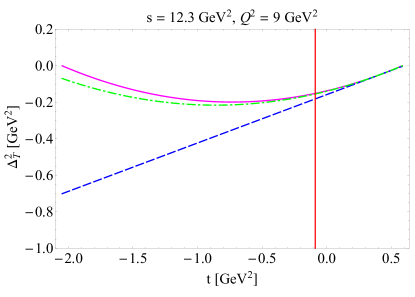
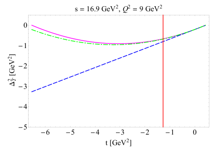
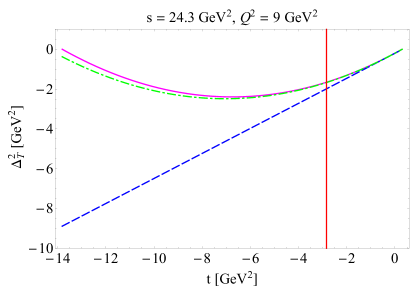
Figure 2: Transverse momentum transfer squared ${(\Delta_{T}^{t})}^{2}$ as the function of $t={(\Delta^{t})}^{2}$ computed from the exact formula in Eq. (9) (solid line) compared to the approximate result of Eq. (4) with $\xi$ expressed by Eq. (6) (dash-dotted line) and approximate expression for $\xi$ in Eq. (7) (dashed line). The functions are drawn for an incident $\bar{p}$ momentum of 5.5 GeV/$c$ (top), 8.0 GeV/$c$ (middle), 12.0 GeV/$c$ (bottom). The minimum value of $t$ for which these approximations are valid is indicated by the solid vertical lines.

Table 1 summarizes the valid ranges of $\Delta^{2}$ in which we are going to apply the factorized description of the reaction (1) for the three selected energies considered here. The lower limit comes from the applicability of collinear factorization (Bjorken limit) for the lowest beam momentum (5.5 GeV/$c$) and from the shortcoming of the approximation employed for the kinematic quantities (kinematic constraints) for the higher two beam momenta (8 and 12 GeV/$c$). The last two columns show how these limits translate to the polar angle of the $\pi^{0}$ in the lab frame, $\theta^{\pi^{0}}_{lab}$, namely the maximum (minimum) valid $\theta^{\pi^{0}}_{lab}$ in the near-forward (near-backward) validity range. At the other end, the minimum (maximum) valid polar angle in the near-forward (near-backward) validity range is $0^{\circ}$ ($180^{\circ}$) for all energies.

Table 1: The kinematic range in which we assume the validity of the factorized description of the signal channel in terms of $\pi N$ TDAs and nucleon DAs for the three values of the incident $\bar{p}$ momentum employed in the present study. The last two columns give the limits in terms of the polar angle of the $\pi^{0}$ in the lab frame for the near-forward and near-backward regimes.

$s$	$p_{\bar{p}}$	$\Delta^{2}_{\min}$	$\Delta^{2}_{\max}$	$\theta^{\pi^{0}}_{lab,\max}$	$\theta^{\pi^{0}}_{lab,\min}$
(GeV2)	(GeV/$c$)	(GeV2)	(GeV2)	Fwd.	Bwd.
12.3	5.5	-0.092	0.59	23.2∘	44.6∘
16.9	8.0	-1.0	0.43	15.0∘	48.1∘
24.3	12.0	-1.0	0.3	7.4∘	62.3∘

III.2 Cross Section Estimates within the Collinear Factorization Approach

The calculation of the $N+\bar{N}\to J/\psi+\pi$ cross section within the collinear factorization approach follows the same main steps as those in the calculations of the $J/\psi\to\bar{p}p$ decay width in the perturbative QCD (pQCD) approach Brodsky and Lepage (1981); Chernyak and Zhitnitsky (1984); Chernyak et al. (1989). The small and large distance dynamics is factorized, and the corresponding amplitude is presented as the convolution of the hard part, computed in the pQCD, with the hadronic matrix elements of the QCD light-cone operators ($\pi N$ TDAs and nucleon DAs) encoding the long distance dynamics (see Fig. 3). The hard scale, which justifies the validity of the perturbative description of the hard subprocess, is provided by the mass of heavy quarkonium $M_{\psi}\simeq 2m_{c}\simeq\bar{M}=3$ GeV.

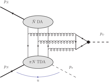
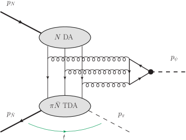
Figure 3: Collinear factorization of the annihilation process $\bar{N}(p_{\bar{N}})N(p_{N})\to J/\psi(p_{\psi})\pi(p_{\pi})$. Top panel: near-backward kinematics ($u\sim 0$). Bottom panel: near-forward kinematics ($t\sim 0$). $\bar{N}(N)$ DA stands for the distribution amplitude of antinucleon (nucleon); $\pi N(\pi\bar{N})$ TDA stands for the transition distribution amplitude from a nucleon (antinucleon) to a pion. Figures reproduced from Ref. Pire et al. (2013).

Within the approximation to order leading twist-three, only the transverse polarization of the $J/\psi$ is relevant, and the cross section with the suggested reaction mechanism for either the near-forward or the near-backward kinematic regimes reads Pire et al. (2013):

$$\frac{d\sigma}{d\Delta^{2}}=\frac{1}{16\pi\Lambda^{2}(s,\ m_{N}^{2},\ m_{N}^{2})}|\overline{\mathcal{M}_{T}}|^{2},$$ (11)

where the squared matrix element $|\overline{\mathcal{M}_{T}}|^{2}$ is expressed as:

$$|\overline{\mathcal{M}_{T}}|^{2}=\frac{1}{4}|\mathcal{C}|^{2}\frac{2(1+\xi)}{\xi{\bar{M}}^{8}}\left(|\mathcal{I}(\xi,\ \Delta^{2})|^{2}-\frac{\Delta_{T}^{2}}{m_{N}^{2}}|\mathcal{I}^{\prime}(\xi,\ \Delta^{2})|^{2}\right).$$ (12)

Here the factor $\mathcal{C}$ reads:

$${\cal C}={(4\pi\alpha_{s})}^{3}\frac{f_{N}^{2}f_{\psi}}{f_{\pi}}\,\frac{10}{81},$$ (13)

where $f_{\pi}=93$ MeV is the pion weak decay constant; $f_{\psi}=(413\pm 8)$ MeV is the normalization constant of the non-relativistic light-cone wave function of heavy quarkonium; $\alpha_{s}$ stands for the strong coupling. The two functions$\mathcal{I}(\xi,\ \Delta^{2})$ and $\mathcal{I}^{\prime}(\xi,\ \Delta^{2})$ denote the convolutions of the hard scattering kernels with the $\pi N$ TDAs and (anti)nucleon DAs. In our studies we employ the estimate of the cross section from Eq. (11) within the simple cross channel nucleon exchange model for the $\pi N$ TDAs Pire et al. (2011). In this model the convolution integrals $\mathcal{I},\mathcal{I}^{\prime}$ read as:

$${\cal I}(\xi,\Delta^{2})=\frac{f_{\pi}\,g_{\pi NN}m_{N}(1-\xi)}{(\Delta^{2}-m_{N}^{2})(1+\xi)}M_{0};$$

$${\cal I}^{\prime}(\xi,\Delta^{2})=\frac{f_{\pi}\,g_{\pi NN}m_{N}}{(\Delta^{2}-m_{N}^{2})}M_{0},$$ (14)

where $f_{N}=(5.0\pm 0.5)$ GeV² is the nucleon wave function normalization constant; $g_{{}_{\pi NN}}\simeq 13$ is the phenomenological pion-nucleon coupling; $M_{0}$ is the standard convolution integral of nucleon DAs occurring in the expression for the $J/\psi\to\bar{p}p$ decay width within the pQCD approach of Ref. Chernyak et al. (1989):

$$\Gamma(J/\psi\to\bar{p}p)={(\pi\alpha_{s})}^{6}\frac{1280f_{\psi}^{2}f_{N}^{4}}{243\pi{\bar{M}^{9}}}|M_{0}|^{2}.$$ (15)

In order to compute the value of the cross section given by Eq. (11), one has to employ the phenomenological solutions for the leading twist nucleon DAs to compute the convolution integral $M_{0}$ and to specify the appropriate value of the strong coupling $\alpha_{s}$ for the characteristic virtuality of the process. Unfortunately, some controversy on this issue exists in recent literature (see e.g. the discussion in Chapter 4 of Ref. Brambilla et al. (2004)). There are several classes of phenomenological solutions for the leading twist nucleon DAs:

• one class (usually referred as the Chernyak-Zhitnitsky-type solutions) contains nucleon DAs which differ considerably from the asymptotic form of the leading twist nucleon DAs. Such DAs require $\alpha_{s}\sim 0.25$ to describe the experimental charmonium decay width $\Gamma(J/\psi\to\bar{p}p)$ from Eq. (15);

• another class of solutions (e.g. the Bolz-Kroll solution Bolz and Kroll (1996) and Braun-Lenz-Wittmann NLO model Braun et al. (2006)) contains nucleon DAs which instead are rather close to the asymptotic form and require $\alpha_{s}\sim 0.4$ to reproduce the experimental $\Gamma(J/\psi\to\bar{p}p)$.

For our rough cross section estimates, intended for the feasibility studies, we follow the prescription from Ref. Pire et al. (2013), and employ the results for the $\bar{p}p\to J/\psi\pi^{0}$ cross section with the value of $\alpha_{s}$ fixed by the requirement that the given phenomenological solution for the nucleon DAs reproduces the experimental $J/\psi\to\bar{p}p$ decay width. In this case the simple nucleon pole model for $\pi N$ TDAs results in the same $\bar{p}p\to J/\psi\pi^{0}$ cross section predictions for any input phenomenological nucleon DA solution.

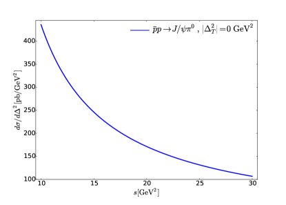
Figure 4: The $s$ dependence of the $\bar{p}p\to J/\psi\pi^{0}$ differential cross section at $|\Delta_{T}^{2}|=0$ GeV/$c^{2}$ as predicted by the calculations based on the TDA formalism given in Ref. Pire et al. (2013).

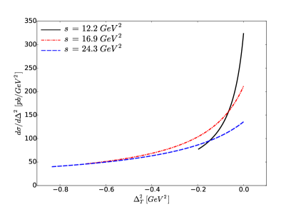
Figure 5: The $\Delta_{T}^{2}$ dependence of the differential cross section predicted by the TDA model for $\bar{p}p\to J/\psi\pi^{0}$ at three incident $\bar{p}$ momenta. The curves have been limited to the validity range of the respective collision energy. The different colored lines show the dependence for the three collision energies considered for the study here: $s~{}=~{}12.3$ GeV² (solid line), $s~{}=~{}16.9$ GeV² (dash-dotted line), $s~{}=~{}25.4$ GeV² (dashed line).

Figure 4 shows the prediction of the $s$ dependence of the differential cross section of $\bar{p}p\to J/\psi\pi^{0}$ at $|\Delta_{T}^{2}|=0$ which decreases only by a factor of about 4 between the lowest to highest CMS collision energies that will be available at $\overline{\mbox{\sf P}}$ANDA. Figure 5 shows the $\Delta_{T}^{2}$ dependence of the cross section for the three collision energies which are used for the studies addressed here, each of them limited to its validity range. It is possible to compare this prediction to the E835 measurement of the $\bar{p}p\to J/\psi\pi^{0}\to e^{+}e^{-}\pi^{0}$ cross section Armstrong et al. (1992); Joffe (2004); Andreotti et al. (2005), taken at an incident $\bar{p}$ momentum of 5.5 GeV/$c$ that corresponds to $s~{}=~{}12.3$ GeV² or $\sqrt{s}~{}=~{}3.5$ GeV. This value of $\sqrt{s}$ is 25 MeV below the threshold for the production of the $h_{c}$ resonance. The reported values lie in the range from 90 pb to 230 pb. Integrating the differential cross section from the TDA model at $s~{}=~{}12.3~{}$GeV² over its validity range ($-0.092<t~{}[$GeV${}^{2}]<0.59$, which is smaller than the full kinematically accessible range), we find 206.8 pb, combining near-forward and near-backward kinematics. This value is on the upper end of the measured range by E835. However, given that the majority of the production rate from the TDA model prediction lies within the validity range, this result gives a degree of confidence that the model can be used as a basis for a feasibility study within its validity range.

Let us stress that the validity of the factorized description of the reaction (1) in terms of $\pi N$ TDAs and nucleon DAs has only been conjectured. The corresponding collinear factorization theorem has never been proven explicitly. Therefore, one of the important experimental challenges is to establish evidence for the validity of this description. In general, there are several essential marking signs for the onset of the collinear factorization regime for a given hard exclusive reaction. The most obvious one is the characteristic scaling behavior of the cross section with the relevant virtuality $1/Q^{2}$. However, for the reaction (1) this feature is of little use, since the virtuality is fixed by the mass of the heavy quarkonium. Another opportunity is to look for the specific polarization dependence. For the case of the nucleon-antinucleon annihilation into $J/\psi$ in association with a forward (or backward) neutral pion it is the transverse polarization of the $J/\psi$ that is dominant within the collinear factorized description in terms of $\pi N$ TDAs. This dominating contribution manifests through the characteristic $(1+\cos^{2}\theta_{\ell}^{*})$ distribution of the decay leptons in the lepton pair CMS scattering angle $\theta_{\ell}^{*}$. The dominance of the corresponding polarization has to be verified by means of a dedicated harmonic analysis.

III.3 Event Generator

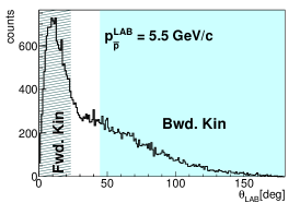
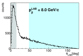
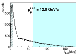
Figure 6: Angular distribution of the $\pi^{0}$ in the lab frame from the event generator based on the TDA formalism in Ref. Pire et al. (2013) at three incident $\bar{p}$ momenta. The validity ranges of the TDA model in terms the lab frame pion emission angle are shown for the near-forward kinematics (hatched) and near-backward kinematics (solid fill).

A Monte Carlo (MC) event generator for the signal reaction was implemented by relying on Eq. (13). The angular distribution of $\pi^{0}$s in the lab frame from this generator is shown in Fig. 6. The entire near-forward kinematic validity range of the reaction is concentrated in a polar angle window below $\approx$ 30^∘ (and even smaller window at higher collision energy), whereas the near-backward kinematic validity range occupies a window above $\approx$ 45^∘ (larger at higher collision energy) extending all the way to $180^{\circ}$. This has implications for the signal reconstruction efficiency as will be shown in Section V.9.

IV Background Properties

In the context of the $\overline{\mbox{\sf P}}$ANDA detector setup, the signal reaction $\bar{p}p\to J/\psi\pi^{0}\to e^{+}e^{-}\pi^{0}$ has multiple background sources with varying degree of importance. These background sources are the subject of discussion in this section. For each source, rate estimates are given and in cases where a full MC is warranted, the details about the event generators that were used to simulate events are presented.

IV.1 Three Pion Production $\bar{p}p\to\pi^{+}\pi^{-}\pi^{0}$

The $\bar{p}p\to\pi^{+}\pi^{-}\pi^{0}$ reaction is an important background source since the cross section is orders of magnitude larger than that of the signal and the possibility to misidentify the charged pion pair as an electron-positron pair. This reaction has been studied in the past at various incident $\bar{p}$ momenta. Despite the limited statistics that were collected, the results from these early measurements tabulated in Ref. Flaminio et al. (1984) provide a valuable benchmark for this study.

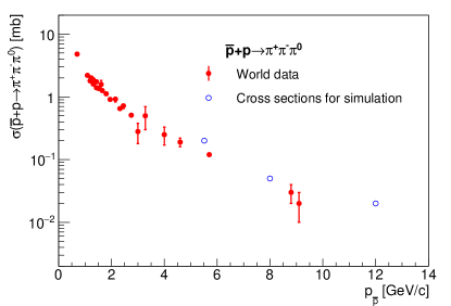
Figure 7: The existing world data of the cross section of $\bar{p}p\to\pi^{+}\pi^{-}\pi^{0}$ (full circles) as reported in Ref. Flaminio et al. (1984), plotted as a function of the incident $\bar{p}$ momentum. The three lab momenta chosen for this study and the corresponding cross sections used in the simulation of this background source are shown as open circles.

As shown in Fig. 7, these results point to a steep decline of the total cross section as a function of incident $\bar{p}$ momentum. For our background simulations, we used total cross sections slightly larger than the interpolation between the nearest existing data points. Very few experiments collected enough statistics to give high quality spectra for this reaction. As a result, the feasibility study relies on the hadronic event generator DPM (Dual Parton Model) Capella et al. (1994) to simulate the shape of the spectra, since the model is constrained by taking into account the sparse experimental differential distributions. In particular, it includes the production of $\rho$ and $f_{2}$ resonances in agreement with experimental observation Bacon et al. (1973).

Table 2 shows the $J/\psi\pi^{0}$ and $\pi^{+}\pi^{-}\pi^{0}$ cross sections in a mass window of 2.8 – 3.3 GeV/$c^{2}$ for the charged pion pair, within the validity ranges of the TDA model (cf. Table 1). The validity range includes both the near-forward and near-backward kinematic approximation zones. The last column of the table gives the approximate signal to background ratio of produced event rates taking into account the $J/\psi\to e^{+}e^{-}$ branching fraction of 5.69%. The ratio of signal to background event production rate is of the order $10^{-7}$ to $10^{-6}$. The fact that the signal $e^{+}e^{-}$ invariant mass distribution is peaked allows to gain a factor of about 10 in signal to background ratio (S/B) before any PID information has been used. The rejection of the rest of the background has to come mostly from PID. The resulting strong requirement on the electron-pion discrimination power will make PID cuts a crucial component of the analysis.

Table 2: Signal ($\bar{p}p\to J/\psi\pi^{0}\to e^{+}e^{-}\pi^{0}$) cross section and production yields, background ($\bar{p}p\to\pi^{+}\pi^{-}\pi^{0}$) cross sections and signal over background ratio. The cross sections have been integrated over the validity range of the model (both near-forward and near-backward). The branching ratio for $J/\psi\to e^{+}e^{-}$ and the mass cut on the $\pi^{+}\pi^{-}$ pair in the range 2.8 – 3.3 GeV/$c^{2}$ have been taken into account. The production yields for the signal are integrated for a luminosity of 2 fb^-1, corresponding to about five months at full luminosity.

$p_{\bar{p}}$	$\Delta\sigma^{J/\psi\pi^{0}}_{valid}$	$N^{e^{+}e^{-}\pi^{0}}_{valid}$	$\Delta\sigma^{\pi^{+}\pi^{-}\pi^{0}}_{valid+m\_cut}$	$S/B_{\pi^{+}\pi^{-}\pi^{0}}$
(GeV/$c$)	(pb)	(2 fb-1)	(mb)
5.5	207	24.6k	8.2$\times$10-3	1.5$\times$10-6
8.0	281	33.3k	1.6$\times$10-3	1.0$\times$10-5
12.0	200	23.7k	3.28$\times$10-4	3.6$\times$10-5

IV.2 Multi-pion Final States ($N_{\pi}\geq 4$)

Multi-pion ($N_{\pi}\geq 4$) final states with at least one $\pi^{+}\pi^{-}$ pair are also potential sources of background to the $\bar{p}p\to J/\psi\pi^{0}\to e^{+}e^{-}\pi^{0}$ channel, if one charged pion pair is misidentified as an $e^{+}e^{-}$ pair. They have cross sections that are up to a factor 15 higher than three pion production, but larger rejection factors can be achieved due to the different kinematics. To confirm this, we performed detailed simulation studies for the $\pi^{+}\pi^{-}\pi^{0}\pi^{0}$ and $\pi^{+}\pi^{-}\pi^{+}\pi^{-}\pi^{0}$ channels, and used the results to conclude on the rejection capability for channels with higher number of pions. The cross sections for the simulation of multi-pion final states is estimated by scaling the $\pi^{+}\pi^{-}\pi^{0}$ cross sections discussed in the previous section, with the scaling factor derived from DPM simulations. Table 3 gives the ratio of cross sections between those multi-pion final states ($\pi^{+}\pi^{-}\pi^{0}\pi^{0}$ and $\pi^{+}\pi^{-}\pi^{+}\pi^{-}\pi^{0}$), and the three-pion final state ($\pi^{+}\pi^{-}\pi^{0}$).

Table 3: The ratio of cross sections of four and five pion final states that could potentially be misidentified as signal to that of the three pion final state, extracted from the DPM hadronic model simulations. The ratios are given at three incident $\bar{p}$ momenta.

$p_{\bar{p}}$ (GeV/$c$)	$\frac{\sigma(\bar{p}p\to\pi^{+}\pi^{-}\pi^{0}\pi^{0})}{\sigma(\bar{p}p\to\pi^{+}\pi^{-}\pi^{0})}$	$\frac{\sigma(\bar{p}p\to\pi^{+}\pi^{-}\pi^{+}\pi^{-}\pi^{0})}{\sigma(\bar{p}p\to\pi^{+}\pi^{-}\pi^{0})}$
5.5	2.9	8.0
8.0	3.2	11.0
12.0	3.4	15.0

IV.3 $\bar{p}p\to J/\psi\pi^{0}\pi^{0}$ with $J/\psi\to e^{+}e^{-}$

For the cross section of the $\bar{p}p\to J/\psi\pi^{0}\pi^{0}\to e^{+}e^{-}\pi^{0}\pi^{0}$ channel, which is not predicted by the DPM model, we assumed a scaling to the $J/\psi\pi^{0}$ channel according to:

$$\frac{\sigma(\bar{p}p\to J/\psi\pi^{0}\pi^{0})}{\sigma(\bar{p}p\to J/\psi\pi^{0})}\approx\frac{\sigma(\bar{p}p\to\pi^{+}\pi^{-}\pi^{0}\pi^{0})}{\sigma(\bar{p}p\to\pi^{+}\pi^{-}\pi^{0})},$$ (16)

where the $\pi^{+}\pi^{-}\pi^{0}\pi^{0}$ to $\pi^{+}\pi^{-}\pi^{0}$ ratios were calculated based on the DPM event generator output. The results for $\bar{p}p\to J/\psi\pi^{0}\pi^{0}\to e^{+}e^{-}\pi^{0}\pi^{0}$ are 35.3 pb, 52.7 pb and 40.7 pb for beam momenta of 5.5 GeV/$c$, 8.0 GeV/$c$ and 12.0 GeV/$c$, respectively. Although there is no existing measurement of the $\bar{p}p\to J/\psi\pi^{0}\pi^{0}$ cross section to confirm these assumptions, we provide arguments below, which suggest that they are reasonably conservative.

The E760 collaboration reported in Ref. Armstrong et al. (1992) the non-observation of a signal for $\bar{p}p\to J/\psi\pi^{0}\pi^{0}\to e^{+}e^{-}\pi^{0}\pi^{0}$ at c.m. energies close to the $h_{c}(1P)$ mass of 3.5 GeV/$c^{2}$. This determines an upper limit for the cross section of 3 pb, which is about a factor 10 below our assumption at this energy. Calculations of non-resonant channels for the $\bar{p}p\to J/\psi\pi^{+}\pi^{-}$ reaction at the $X(3872)$ energy have been performed with an hadronic model Chen and Ma (2008), yielding a cross section of about 60 pb for $\bar{p}p\to J/\psi\pi^{+}\pi^{-}\to e^{+}e^{-}\pi^{+}\pi^{-}$ at $\sqrt{s}$ around 3.872 GeV. With the assumption of a factor two smaller cross section for $\bar{p}p\to J/\psi\pi^{0}\pi^{0}\to e^{+}e^{-}\pi^{0}\pi^{0}$ based on isospin coefficients, this calculation is consistent with our assumption. These calculations, outlined in Ref. Chen and Ma (2008), are however likely to have been overestimated due to the absence of vertex cut-off form factors, as in Ref. Van de Wiele and Ong (2013) for the case of $\bar{p}p\to J/\psi\pi^{0}$. Finally, the cross section for the production of the $\bar{p}p\to J/\psi\pi^{0}\pi^{0}\to e^{+}e^{-}\pi^{0}\pi^{0}$ channel via feed-down from a resonance might in some cases be expected to be lower than, or of the same magnitude, as our assumptions. This is obviously the case for resonances with charge conjugation $C=1$, e.g. the $X(3872)$, which do not decay into $J/\psi$ plus any number of $\pi^{0}$s. But charmonium states with $C=1$ might also contribute to the $J/\psi\pi^{0}\pi^{0}$ channel with cross sections that are lower or of the same order of magnitude. For example, a prediction of 30 pb for the reaction $\bar{p}p\to Y(4260)\to J/\psi\pi^{0}\pi^{0}\to e^{+}e^{-}\pi^{0}\pi^{0}$ at $\sqrt{s}=4.260$ GeV was provided in Ref. Erni et al. (2009), with the assumption that, having the same quantum numbers as the $\psi(2S)$, the $Y(4260)$ decays into $J/\psi\pi^{0}\pi^{0}$ with the same branching ratio as what was reported in Ref. Negrini (2004). The $Y(4260)$ resonance will probably have a very low branching fraction for decays into the $J/\psi\pi^{0}$ and $\pi^{+}\pi^{-}\pi^{0}$ channels, and will therefore not contribute significantly to the signal and to the other backgrounds.

IV.4 Di-electron Continuum: $\bar{p}p\to\gamma^{*}\pi^{0}\to e^{+}e^{-}\pi^{0}$

The production of a $\gamma^{*}$ with an associated $\pi^{0}$ is another process which can be used to demonstrate the universality of the TDAs Singh et al. (2015). When the invariant mass of the electron-positron pair is near the $J/\psi$ mass, this channel represents a background source to the $\bar{p}p\to J/\psi\pi^{0}\to e^{+}e^{-}\pi^{0}$ channel, which can not be rejected in the analysis procedure since the particles in final state are identical to the signal. A similar TDA formalism to the one used here for the prediction of the $J/\psi\pi^{0}$ channel can also be used to estimate the differential cross section for $\bar{p}p\to\gamma^{*}\pi^{0}\to e^{+}e^{-}\pi^{0}$, as demonstrated in Ref. Singh et al. (2015). The same predictions can be used to integrate the cross section numerically over the corresponding validity domains at each collision energy (cf. Table 1).

After setting the range $8.4<Q^{2}~{}[GeV^{2}]<10.1$ to match the window around the $J/\psi$ mass, which will be used for the analysis, cross sections of 13.6 fb, 21.6 fb and 24.8 fb are obtained at $s~{}=~{}$12.3 GeV², $s~{}=~{}$16.9 GeV² and $s~{}=~{}$24.3 GeV², respectively. Taking into account the branching ratio of $J/\psi\to e^{+}e^{-}$ (5.94%), this results in contamination on the $10^{-3}$ level and therefore has not been considered for further simulations.

IV.5 Hadronic Decays of $J/\psi$

The reaction $\bar{p}p\to J/\psi\pi^{0}$, with the $J/\psi$ decaying into $\pi^{+}\pi^{-}$, where the $\pi^{+}\pi^{-}$ pair is subsequently misidentified as a $e^{+}e^{-}$ pair, is another potential source of background. It is highly suppressed by the branching fraction of $J/\psi$ into $\pi^{+}\pi^{-}$ ($\approx~{}10^{-4}$), and the low probability of misidentifying the pions as electrons (cf. Section V.2).

Similarly, $\bar{p}p\to J/\psi\pi^{0}$ events with a hadronic $J/\psi$ decay that can mimic the signal’s final state (for example $J/\psi\to\pi^{+}\pi^{-}\pi^{0}$ or $J/\psi\to\gamma\pi^{+}\pi^{-}$) is heavily suppressed by the probability to identify the $\pi^{+}\pi^{-}$ pair. With the same production cross sections as the signal, and with very low probability of misidentifying the $\pi^{+}\pi^{-}$ pair as an $e^{+}e^{-}$ pair, such final states have negligible detection rates, and therefore will not be fully simulated.

V Simulations and Analysis

For the present feasibility study, full MC simulations were performed on events from both the signal and background event generators described in the previous sections. In this section details of the analysis procedure will be provided. After a brief overview of the analysis methodology, a discussion of the PID and selection procedure, the reconstruction of $\pi^{0}$ and $e^{+}e^{-}$ pairs, as well as the use of kinematic fits to gain further rejection for one class of background reaction where PID alone is not sufficient is provided. The section concludes with global signal to background ratios and signal purity for each background type included in the simulation study.

V.1 Brief Description of the Method

The analysis starts with the generation of signal and background events as described in Section III, followed by the transport of tracks in GEANT4, where the geometry of the $\overline{\mbox{\sf P}}$ANDA detector has been implemented. The simulation of the detector response and digitization of the signals follows this step, at which point tracks and neutral particles can be reconstructed.

Signal events are then passed to the full event selection chain, including PID and analysis cuts. This ensures the most realistic description possible of the reconstructed signal, including statistical fluctuations. The number of signal events to simulate was picked to correspond exactly to the expected signal counts shown in Table 2 within the validity domain. By directly plotting spectra with tracks that pass all identification cuts, the plots will reflect the expected statistical accuracy.

For the background events, a different approach was followed. To check the feasibility of the measurement, the residual background contamination needs to be understood with a good precision in each bin used for the extraction of the physics observable (e.g. differential cross section distribution in $t$). This would not be possible if the cuts are directly applied due to the small number of background events that would pass all cuts. Therefore, a weight proportional to the product of single charged track misidentification probabilities is applied to each event instead of direct application of cuts as in the case of signal event simulation. The charged pion misidentification probability is parameterized as a function of momentum of the track. The photon selection is done by direct application of the cuts, just as in the case of the signal event analysis.

Figure 8 shows the polar angle versus momentum distributions of reconstructed final state tracks in the background (top row) and signal (bottom row) simulations at the three different $\bar{p}$ incident momenta used in this study.

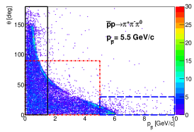
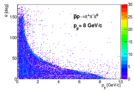
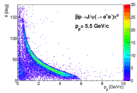
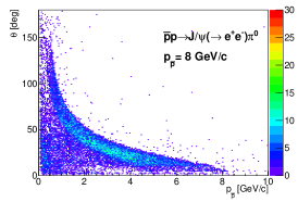
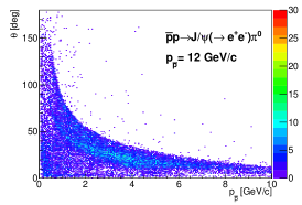
Figure 8: The polar angle vs momentum distribution of reconstructed single charged tracks in full MC simulation of the background (top row) and signal (bottom row) event generator output. The simulations were performed at the three $\bar{p}$ incident momenta chosen for this study. The boxes in the top left panel show the regions in which high statistics flat single track simulations were generated for low (full line), intermediate (dash-dotted line) and high (dashed line) momentum tracks for use in the efficiency and rejection studies.

V.2 PID Efficiency

For the investigation of PID efficiency, single particle simulations of electrons, positrons, positive and negative pions were performed in the three kinematic zones depicted by red, black and blue boxes in Fig. 8. This is to focus the simulation to values of $p$ and $\theta$ that matter most for this study. In total, $5\times 10^{6}$ single $e^{+}$ and $e^{-}$ events each were used for the estimation of the electron efficiency. To obtain a good precision on the very low pion misidentification probability, a larger statistics of $25\times 10^{6}$ each for single $\pi^{+}$ and $\pi^{-}$ events were used. The following section discusses in more detail how these efficiencies were determined. For the sake of simplicity in the remainder of the discussion, the word electron is used to refer to both electrons and positrons, except when the distinction is necessary.

As mentioned above, one of the critical aspects of this analysis is the reduction of the hadronic background using PID cuts, since the $\pi^{+}\pi^{-}\pi^{0}$ final state is kinematically very similar to the $J/\psi\pi^{0}\to e^{+}e^{-}\pi^{0}$ final state when the $\pi^{+}\pi^{-}$ invariant mass is close to the $J/\psi$ invariant mass. To this end, the PID should be used in the most effective way possible to maximize pion rejection until the cost to electron efficiency is prohibitive. This section describes the selection cuts of the analysis.

V.2.1 Combined PID Probability

The starting point for the application of global PID is the detector-by-detector PID probability information. To simplify the process of combining information from various detectors, the relevant PID variables from a given detector subsystem $i\in\{subsys\}=\{\mathrm{EMC},\mathrm{DIRC},\mathrm{DISC},\mathrm{STT},\mathrm{MVD}\}$ is used to determine an estimate of the probability $\mathcal{P}^{ID}_{i}(j)$ that a given track is one of the five charged particles species that can be identified by $\overline{\mbox{\sf P}}$ANDA, where $j\in\{e^{\pm},\ \mu^{\pm},\ \pi^{\pm},\ K^{\pm},\ p^{\pm}\}$. The combined probability that a given track is of type $j$ is then given by:

$$\mathcal{P}^{ID}_{comb}(j)=\frac{\mathcal{P}^{ID}(j)}{1+\mathcal{P}^{ID}(j)},$$ (17)

where:

$$\mathcal{P}^{ID}(j)=\prod_{i\in\{subsys\}}\frac{\mathcal{P}^{ID}_{i}(j)}{1-\mathcal{P}^{ID}_{i}(j)}.$$ (18)

Equation (17) ensures the proper normalization of the probabilities assigned for each track: $\sum_{j}{\mathcal{P}^{ID}_{comb}(j)}=1$. With the combined probability in hand, a cut is applied at an appropriate value for the identification of any given species. In the present case, a sufficiently high threshold on $\mathcal{P}^{ID}_{comb}(e^{\pm})$ is imposed to select electrons and reject all other species. Here we show in Fig. 9 the global PID efficiency $\varepsilon_{eid}^{e^{\pm}}(\theta_{MC},\ p_{MC})$ as a function of the true MC polar angle $\theta_{MC}$ and momentum $p_{MC}$ with a cut of $\mathcal{P}^{ID}_{comb}(e^{\pm})>0.9$, based on a simulation of $10^{7}$ electrons and positrons. Figure 10 shows the pion misidentification probability $\varepsilon_{eid}^{\pi^{\pm}}(p_{MC})$ as a function of $p_{MC}$ for the same cut based on a simulation of $5\times 10^{7}$ charged pions.

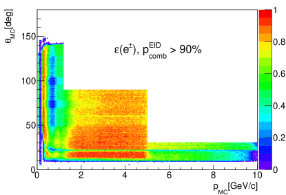
Figure 9: The EID efficiency with a probability threshold of 90% for electrons and positrons as a function of MC polar angle $\theta_{MC}$ and MC momentum $p_{MC}$.

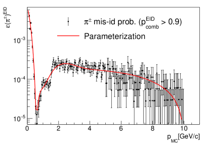
Figure 10: Misidentification probability for charged pions as a function of true MC momentum for a combined EID probability threshold of 90%. The efficiency parameterization is shown by the full line.

V.2.2 Optimization of the Cut on $\mathcal{P}^{ID}_{comb}(e^{\pm})$

To determine an optimal cut on $\mathcal{P}^{ID}_{comb}(e^{\pm})$ for EID, the relationship between average efficiency of EID $\varepsilon(e^{\pm})$ versus average misidentification probability for charged pions $\varepsilon(\pi^{\pm})$ was studied as a function of the cut on $\mathcal{P}^{ID}_{comb}(e^{\pm})$, and plotted in Fig. 11 as a ROC (Receiver Operating Characteristics) curve, which shows the performance of the classifier as the discrimination threshold is varied. $\varepsilon(e^{\pm})$ and $\varepsilon(\pi^{\pm})$ are determined by taking the bin-by-bin weighted average of the electron efficiency shown in Fig. 9 and pion misidentification probability shown in Fig. 10. The weight for each bin is set to the content of the corresponding bin in the kinematic distributions shown in Fig. 8. One can observe that there is a significant gain in charged pion rejection with relatively small loss in EID efficiency up to a cut of $\mathcal{P}^{ID}_{comb}(e^{\pm})>90\%$, beyond which the rejection gain no longer justifies the associated loss in efficiency. The cut of $\mathcal{P}^{ID}_{comb}(e^{\pm})>90\%$ is therefore chosen for the remainder of this analysis. It should be noted that the difference of the ROC curves between different incident $\bar{p}$ momenta comes from the differences in the momentum and angular distributions of single tracks in the signal and background events that were used as a weight to average the efficiencies bin by bin.

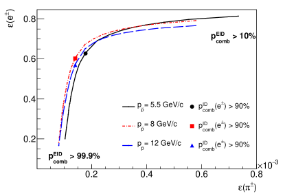
Figure 11: ROC curves for $\mathcal{P}^{ID}_{comb}(e^{\pm})$ cuts showing the efficiency to identify an electron vs the probability to misidentify charged pions at the three different $\bar{p}$ incident momenta, 5.5 GeV/$c$ (solid line), 8.0 GeV/$c$ (dash-dotted line) and 12.0 GeV/$c$ (dashed line). The full points with the corresponding color show the efficiencies and misidentification probabilities for $\mathcal{P}^{ID}_{comb}(e^{\pm})~{}>~{}90\%$ at the respective beam momenta.

V.2.3 Application of the $\mathcal{P}^{ID}_{comb}(e^{\pm})$ Cut

The application of the cut on $\mathcal{P}^{ID}_{comb}(e^{\pm})$ is straightforward for the signal simulations. The cut is applied on a track-by-track basis to every reconstructed electron, and the spectra are constructed from those tracks that pass the cut. This approach is however not realistic for the background simulations, since the rejection is very high ($\approx~{}10^{-4}$ per charged pion). An unrealistically large number of background events need to be simulated to produce sufficient statistics in each bin after all cuts are applied. For this reason a different approach is adopted. The single pion misidentification probability shown in Fig. 10 is parameterized by a function $f^{\varepsilon}_{\pi^{\pm}}(p)$ to smooth out the statistical fluctuation, and subsequently used as a weight for each background event based on the product of the values of $f^{\varepsilon}_{\pi^{\pm}}(p)$ at the respective true MC momenta of the two identified pions, $p_{\pi^{+}}$ and $p_{\pi^{+}}$:

$$w(p_{\pi^{+}},p_{\pi^{-}})=\frac{N^{BG}}{N^{MC}_{evt}}f^{\varepsilon}_{\pi^{\pm}}(p_{\pi^{+}})f^{\varepsilon}_{\pi^{\pm}}(p_{\pi^{-}}),$$ (19)

where $N^{MC}_{evt}$ is the number of full $\bar{p}p\to\pi^{+}\pi^{-}\pi^{0}$ reaction events that were simulated, and $N^{BG}$ is the number of background events that are expected from 2 fb^-1 integrated luminosity based on the cross sections given in column 4 of Table 2. The constant factor $N^{BG}/N^{MC}_{evt}$ ensures the proper normalization of the background spectra.

V.3 $\pi^{0}$ Reconstruction

Neutral pions are reconstructed through their two-photon decay channel, in the invariant mass spectrum formed by combining all photons within an event into $\gamma\gamma$ pairs. A cluster from the EMC with a minimum reconstructed energy of 3 MeV is considered to originate from a photon if there is no charged track candidate whose extrapolation to the EMC falls within a 20 cm radius from the EMC cluster. The invariant mass spectra show a contribution from combinatorial $\gamma\gamma$ pairs, which can be reduced by relying on the kinematic correlation of $\pi^{0}$ decay photons that the combinatorial $\gamma\gamma$ pairs do not display.

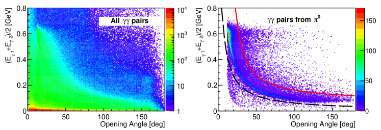
Figure 12: The average reconstructed energy of a photon pair versus its opening angle for all $\gamma\gamma$ pairs within an event (left panel) compared to $\gamma\gamma$ pairs stemming from $\pi^{0}$ decay (right panel), in a simulation of $\bar{p}p\to J/\psi\pi^{0}\to e^{+}e^{-}\pi^{0}$ events at $p_{\bar{p}}=$ 5.5 GeV/$c$. The full and dashed lines in the right panel show the upper and lower bounds of the cut described in Eq. (20), with $a^{L}_{0}=0$, $a^{L}_{1}=0.11$, $a^{L}_{2}=-0.05$, $a^{U}_{0}=0.07$, $a^{U}_{1}=0.14$, and $a^{U}_{2}=0.21$.

Figure 12 shows the correlation of the reconstructed average photon energy to the opening angle in the lab frame between two photons, from all $\gamma\gamma$ pairs including those from combinatorial pairs on the left, and for $\gamma\gamma$ pairs that decay from a $\pi^{0}$ on the right, in $\bar{p}p\to J/\psi\pi^{0}\to e^{+}e^{-}\pi^{0}$ events simulated within the validity domains of the TDA model.

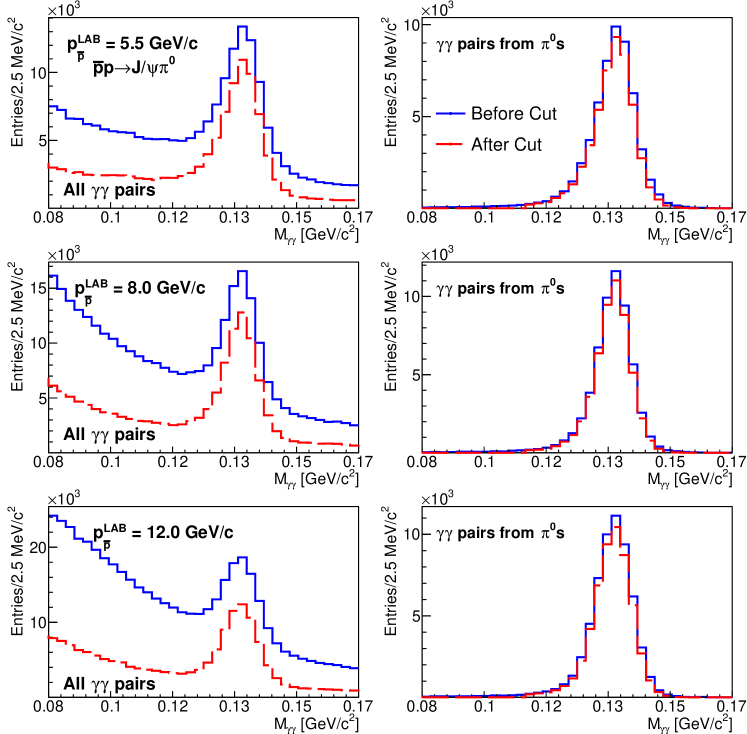
Figure 13: Two photon invariant mass spectra for the signal reaction $\bar{p}p\to J/\psi\pi^{0}\to e^{+}e^{-}\pi^{0}$. The left column shows the invariant mass spectra for all $\gamma\gamma$ pairs in the event, before the cut given by Eq. (20) (solid line) and after the cut (dashed line). The right column shows the corresponding invariant mass distributions for reconstructed photon pairs from $\pi^{0}$ decay. Each row corresponds to a different $\bar{p}$ incident momentum: 5.5 GeV/$c$ (top row), 8.0 GeV/$c$ (middle row) and 12.0 GeV/$c$ (bottom row).

The following cuts are applied to the data:

$$f_{L}(OA)\ <\ \frac{E_{\gamma 1}+E_{\gamma 2}}{2}\ <\ \begin{cases}\infty\ \ \ (OA\leq a^{U}_{2})\\ f_{U}(OA)\ \ \ (OA>a^{U}_{2})\end{cases}$$ (20)

with:

$$f_{L}(x)=a^{L}_{0}+\frac{a^{L}_{1}}{x-a^{L}_{2}},\ \ and\ \ f_{U}(x)=a^{U}_{0}+\frac{a^{U}_{1}}{x-a^{U}_{2}},$$

where OA is the opening angle between the two photons, $E_{\gamma 1}$ and $E_{\gamma 2}$ are the energies of the two photons, and $a^{L}_{i}$ and $a^{U}_{i}$, with $i=0,1,2$ are coefficients of the parametrization determined independently for each collision energy. Thus, it is possible to reduce the combinatorial background to a few percent while keeping an efficiency larger than 90% for pairs where both photons stem from $\pi^{0}$ decays. The effect of this cut is shown in Fig. 13 in a simulation of $\bar{p}p\to J/\psi\pi^{0}\to e^{+}e^{-}\pi^{0}$ events, for all photon pairs on the left and for photons originating from $\pi^{0}$ decays on the right. In addition to this, an invariant mass cut of 110 $<~{}m_{\gamma\gamma}~{}<$ 160 MeV/c² is applied on the two photon system.

V.4 $J/\psi$ Reconstruction

The reconstruction of $J/\psi$ candidates is accomplished by pairing all positive charged candidates passing EID cuts with all negative charged candidates that also pass the EID cuts. Figure 14 shows the invariant mass spectrum of $e^{+}e^{-}$ pairs after application of the EID cuts, while requiring the presence of at least one reconstructed $\pi^{0}$ in the event. The mass distribution can be described satisfactorily by a Crystal Ball function Oreglia (1980). A fit to the mass distribution has a peak at $(3.088\pm 0.001)$ GeV/$c^{2}$ and a width of $(51.3\pm 1.0)$ MeV/$c^{2}$. The solid vertical lines show the mass window 2.8 $<$ $M_{e^{+}e^{-}}$ $<$ 3.3 GeV/$c^{2}$ which is used as a selection to reconstruct $e^{+}e^{-}$ pairs from $J/\psi$.

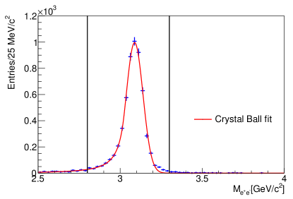
Figure 14: $e^{+}e^{-}$ invariant mass spectrum (data points) fit with a Crystal Ball function (solid line) for the reaction $\bar{p}p\to J/\psi\pi^{0}\to e^{+}e^{-}\pi^{0}$ at a beam momentum of $p_{\bar{p}}=$ 5.5 GeV/$c$. The solid vertical lines denote the 2.8 < $M_{e^{+}e^{-}}$ [GeV/$c^{2}$] $<$ 3.3 mass window used in this analysis for the selection of $J/\psi$ candidates.

V.5 $J/\psi\pi^{0}$ Signal Reconstruction

Finally, the full event is reconstructed by pairwise combining all reconstructed $\pi^{0}$s with all $J/\psi$ candidate $e^{+}e^{-}$ pairs in the same event. Due to the presence of combinatorial background in both the $\pi^{0}$ reconstruction (random $\gamma\gamma$ pairs) and the $J/\psi$ reconstruction (random $e^{+}e^{-}$ pairs), there could be more than one candidate $J/\psi\pi^{0}$ pair per event. In such events, the angle between the $\pi^{0}$ and $J/\psi$ in the CMS is calculated for each pair and the combination closest to 180^∘ (the most back-to-back pair) is selected. Figure 15 depicts the invariant mass distributions of the signal reaction as well as all the simulated background sources after the selection of the $\pi^{0}$ and $e^{+}e^{-}$ pair. The sum of contributions (S+B) from signal (S) and all background sources (B) is shown in the same figure as the black histogram.

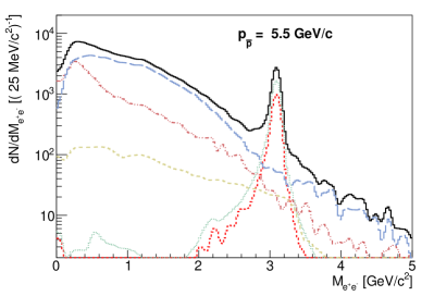
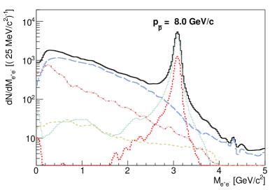
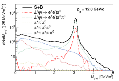
Figure 15: Dilepton invariant mass distributions of the simulated signal and background sources after selection of one $\pi^{0}$ and one $e^{+}e^{-}$ pair. The three beam momenta used for this study are shown: 5.5 GeV/$c$ (top panel), 8.0 GeV/$c$ (middle panel) and 12.0 GeV/$c$ (bottom panel). Individual contributions from the various sources of background discussed in the text are also plotted with the line style depicted in the legend. $\pi^{+}\pi^{-}\pi^{0}$, $\pi^{+}\pi^{-}\pi^{0}\pi^{0}$ and $\pi^{+}\pi^{-}\pi^{+}\pi^{-}\pi^{0}$ are generated using DPM, whereas $J/\psi\pi^{0}\pi^{0}$ is generated using the phase-space (PHSP) model. The combined contribution (S+B) of the signal (S) and all background (B) reactions is shown by the solid line. Events of the signal channel $J/\psi\pi^{0}$ are generated using the TDA model-based generator.

Table 4 shows the signal to background ratios of the different background sources simulated at this stage of the analysis, and the first column of Table 5 displays the efficiency of the signal and the rejection powers of different sources of background. The channels with a charged pion pair are suppressed with rejection powers of the order 10⁷. The main effect (roughly $10^{6}$) comes from PID, while the remaining factor of $10$ comes from the cut on the charged pair invariant mass. As a result, background events can be rejected to levels where they can be subtracted when needed in the $e^{+}e^{-}$ invariant mass spectra by a sideband analysis, in which invariant mass regions to the right and left side of the $J/\psi$ peak are used to estimate the background contribution under the peak. This is discussed in more detail in Section V.8. As expected, the $J/\psi\pi^{0}\pi^{0}$ channel is selected with an efficiency similar to the $J/\psi\pi^{0}$ channel. It is therefore now the dominant background source, roughly a factor four larger than the signal. This ratio is a direct result of the conservatively high cross section assumption discussed in Section IV.3. A dedicated analysis of the $J/\psi\pi^{0}\pi^{0}$ channel will be possible with $\overline{\mbox{\sf P}}$ANDA, allowing for measurement of the cross section at the same c.m energy as the $J/\psi\pi^{0}$ signal. In the mean time, we stick to the cross section inputs as described in Section IV.3, and propose further analysis cuts described in the following section to reduce this background to the percent level, keeping in mind that that they will later be adjusted to match realistic values of the $J/\psi\pi^{0}\pi^{0}$ cross section.

Table 4: Signal to background ratio for different background sources after selection of one $\pi^{0}$ and one $e^{+}e^{-}$ pair. The signal (S) and background (B) are counted within a window of 2.8 to 3.3 GeV/$c^{2}$ in the invariant mass of the charged pair, and inside the validity range of the TDA model.

S/B	5.5 GeV/$c$	8.0 GeV/$c$	12.0 GeV/$c$
$J/\psi\pi^{0}\pi^{0}$	0.273	0.251	0.225
$\pi^{+}\pi^{-}\pi^{0}$	12.6	56.4	366.0
$\pi^{+}\pi^{-}\pi^{0}\pi^{0}$	10.3	24.9	101.0
$\pi^{+}\pi^{-}\pi^{+}\pi^{-}\pi^{0}$	4.8	6.76	15.6
combined	0.247	0.239	0.221

V.6 Kinematic Fit

The $J/\psi\pi^{0}\pi^{0}$ background will be reduced by exploiting the kinematic differences to the $J/\psi\pi^{0}$ channel. Figure 16 shows the $\chi^{2}$ distributions of a kinematic fit with four-momentum conservation enforced as a constraint by assuming an exclusive $\gamma\gamma e^{+}e^{-}$ event (denoted as $\chi^{2}_{2\gamma e^{+}e^{-}}$). The plots are shown for the three beam momenta of this study. The insets show the same plot on a linear scale with a restricted range on the $\chi^{2}$ axis, demonstrating that $\chi^{2}_{2\gamma e^{+}e^{-}}$ is peaked at values compatible with the four degrees of freedom of the kinematic fit to the $\bar{p}p\to J/\psi\pi^{0}$ hypothesis. In contrast, the $J/\psi\pi^{0}\pi^{0}$ events show a significantly flatter $\chi^{2}_{2\gamma e^{+}e^{-}}$ distribution extending to very large values, providing a powerful tool for further rejection. As shown in the second column of Table 5, by applying a maximum cut-off on $\chi^{2}_{2\gamma e^{+}e^{-}}$ of 20, 50 and 100 at $p_{\bar{p}}=$ 5.5, 8.0 and 12.0 GeV/$c$, respectively, it is possible to reduce the $J/\psi\pi^{0}\pi^{0}$ contamination to less than 8%, while keeping the corresponding loss in signal efficiency to $\approx$ 15 – 30%, depending on $p_{\bar{p}}$.

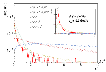
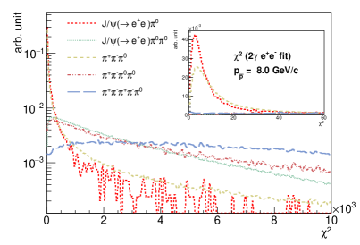
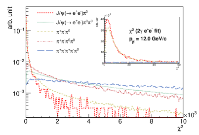
Figure 16: The $\chi^{2}$ distribution of the kinematic fit (main plot). The inset shows a small region of $\chi^{2}$ with a linear scale. The three plots represent the different beam momenta studies, 5.5 GeV/$c$ (top), 8.0 GeV/$c$ (center) and 12.0 GeV/$c$ (bottom). The different distributions represent the signal and four sources of background simulated for the feasibility study. The distributions are normalized to have the same integral for easier comparison.

Despite the significant improvement of the S/B ratio, additional cuts are needed to bring the contamination by $J/\psi\pi^{0}\pi^{0}$ to under a few percent at all energies. A comparison of the $\chi^{2}$ value of the kinematic fit for the $2\gamma e^{+}e^{-}$ hypothesis ($\chi^{2}_{2\gamma e^{+}e^{-}}$) with the $\chi^{2}$ value for the $4\gamma e^{+}e^{-}$ hypothesis ($\chi^{2}_{4\gamma e^{+}e^{-}}$) can provide additional discrimination power. The correlation between $\chi^{2}_{2\gamma e^{+}e^{-}}$ and $\chi^{2}_{4\gamma e^{+}e^{-}}$ is shown in Fig. 17. By requiring $\chi^{2}_{4\gamma e^{+}e^{-}}~{}>~{}\chi^{2}_{2\gamma e^{+}e^{-}}$ for those reconstructed $J/\psi\pi^{0}$ events with an additional $\gamma\gamma$ pair in the event lowers the $J/\psi\pi^{0}\pi^{0}$ contamination down to less than 5%, depending on $p_{\bar{p}}$, with no significant loss in signal efficiency.

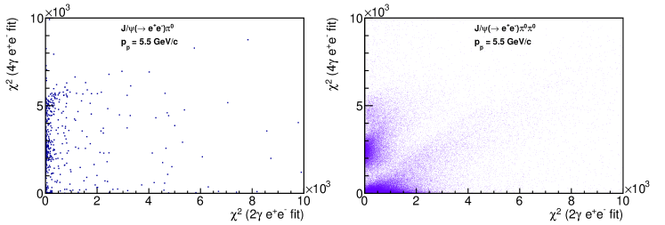
Figure 17: The correlation between $\chi^{2}_{2\gamma e^{+}e^{-}}$ and $\chi^{2}_{4\gamma e^{+}e^{-}}$ for $J/\psi\pi^{0}$ (left) and $J/\psi\pi^{0}\pi^{0}$ (right) events at beam momentum of $p_{\bar{p}}=$ 5.5 GeV/$c$.

Finally, by requiring that the number of photons in the event with energy above 20 MeV ($N_{\gamma(>20MeV)}$, shown in Fig. 18 for $J/\psi\pi^{0}$ and $J/\psi\pi^{0}\pi^{0}$ events) to be less than or equal to three, it is possible to achieve a $J/\psi\pi^{0}\pi^{0}$ contamination of less than 2% with an additional loss of efficiency of only about 10 – 15%.

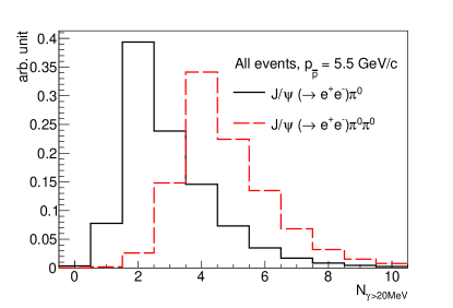
Figure 18: Distribution of the number of photons above 20 MeV per event for the $J/\psi\pi^{0}$ signal (solid line) and $J/\psi\pi^{0}\pi^{0}$ background (dashed line) channels at beam momentum of $p_{\bar{p}}=$ 5.5 GeV/$c$.

Table 5 summarizes key quantities, signal efficiency, contamination from $J/\psi\pi^{0}\pi^{0}$ and $\pi^{+}\pi^{-}\pi^{0}$ and purity from combinatorial background as well as S/B ratio including all background sources after each step in the analysis procedure described above, starting from the $e^{+}e^{-}\pi^{0}$ selection.

Table 5: The efficiency for signal events and rejection factor ($\mathcal{R}$) of the two significant background contributions, together with background contamination ($\mathcal{C}$), signal purity from combinatorial background ($\mathcal{P}_{comb}$) and total signal to background ratio. The quantities are tabulated with successive application of kinematic cuts starting from the selection of the $\pi^{0}$ and $e^{+}e^{-}$ pair (column $e^{+}e^{-}\pi^{0}$ sel.). The signal and background count rates are determined within a $M_{e^{+}e^{-}}$ window of 2.8 to 3.3 GeV/$c^{2}$ in the invariant mass of the charged pair. The beam momentum for each table is given in the top left cell.

5.5 GeV/$c$	$e^{+}e^{-}\pi^{0}$ sel.	$\chi^{2}_{2\gamma e^{+}e^{-}}$	$\chi^{2}_{4\gamma e^{+}e^{-}}$	$N_{\gamma(>20MeV)}$
$\varepsilon_{\bar{p}p\to J/\psi\pi^{0}}$	17.8%	12.5%	12.5%	11.3%
$\mathcal{R}_{J/\psi\pi^{0}\pi^{0}}$	4.5	360	590	1.6$\times 10^{3}$
$\mathcal{R}_{\pi^{+}\pi^{-}\pi^{0}}$	9.0$\times 10^{8}$	1.8$\times 10^{9}$	1.8$\times 10^{9}$	2.9$\times 10^{9}$
$\mathcal{C}_{J/\psi\pi^{0}\pi^{0}}$	441.9%	7.5%	4.5%	1.8%
$\mathcal{C}_{\pi^{+}\pi^{-}\pi^{0}}$	6.6%	4.9%	4.9%	3.4%
$\mathcal{P}_{comb}$	90.4%	98.8%	98.8%	99.0%
$S/B$	0.2	7.7	10.1	19.6
8.0 GeV/$c$	$e^{+}e^{-}\pi^{0}$ sel.	$\chi^{2}_{2\gamma e^{+}e^{-}}$	$\chi^{2}_{4\gamma e^{+}e^{-}}$	$N_{\gamma(>20MeV)}$
$\varepsilon_{\bar{p}p\to J/\psi\pi^{0}}$	15.5%	12.2%	12.2%	10.5%
$\mathcal{R}_{J/\psi\pi^{0}\pi^{0}}$	5.2	650	1.4$\times 10^{3}$	3.8$\times 10^{3}$
$\mathcal{R}_{\pi^{+}\pi^{-}\pi^{0}}$	7.6$\times 10^{8}$	1.3$\times 10^{9}$	1.3$\times 10^{9}$	2.2$\times 10^{9}$
$\mathcal{C}_{J/\psi\pi^{0}\pi^{0}}$	456.4%	3.4%	1.7%	0.8%
$\mathcal{C}_{\pi^{+}\pi^{-}\pi^{0}}$	1.5%	1.2%	1.2%	0.8%
$\mathcal{P}_{comb}$	89.3%	98.7%	98.7%	99.0%
$S/B$	0.2	19.6	33.7	67.5
12.0 GeV/$c$	$e^{+}e^{-}\pi^{0}$ sel.	$\chi^{2}_{2\gamma e^{+}e^{-}}$	$\chi^{2}_{4\gamma e^{+}e^{-}}$	$N_{\gamma(>20MeV)}$
$\varepsilon_{\bar{p}p\to J/\psi\pi^{0}}$	9.4%	7.9%	7.9%	6.6%
$\mathcal{R}_{J/\psi\pi^{0}\pi^{0}}$	7.7	6.8	1.8$\times 10^{3}$	5.3$\times 10^{3}$
$\mathcal{R}_{\pi^{+}\pi^{-}\pi^{0}}$	1.4$\times 10^{9}$	2.1$\times 10^{9}$	2.1$\times 10^{9}$	4.0$\times 10^{9}$
$\mathcal{C}_{J/\psi\pi^{0}\pi^{0}}$	413.2%	4.0%	1.2%	0.6%
$\mathcal{C}_{\pi^{+}\pi^{-}\pi^{0}}$	0.2%	0.1%	0.1%	0.1%
$\mathcal{P}_{comb}$	89.1%	99.7%	98.8%	99.0%
$S/B$	0.2	21.9	57.9	159.3

V.7 Signal to Background Ratio

The expected background contamination from all sources considered in this study is plotted in Fig. 19 as the shaded histogram for each validity range at the three beam momenta. In the worst scenario (at the lowest energy studied here at $p_{\bar{p}}=$ 5.5 GeV/$c$), the S/B ratio will be at least of the order of 15 at all values of $t$. At higher energies, the background contamination from $\bar{p}p\to\pi^{+}\pi^{-}\pi^{0}$ is about or less than a percent, even with the conservative estimates of the background cross section used. As already mentioned, $\overline{\mbox{\sf P}}$ANDA will provide dedicated measurements of these background channels, hence allowing for a subtraction of the corresponding contributions. In addition, background channels with no $J/\psi$ in the final state can be suppressed using a sideband analysis of the invariant mass distribution of the charged pair, as will be discussed in the next section. This gives us confidence that the measurement should be readily feasible from the point of view of background rejection.

V.8 Sideband Background Subtraction

The number of reconstructed signal events is extracted by subtracting the background contribution from the total number of entries within the range 2.8 $<$ $M_{e^{+}e^{-}}$ $<$ 3.3 GeV/$c^{2}$. The background contribution is obtained by integrating the polynomial component of the Crystal Ball (see Section V.4) plus third order polynomial function fitted to the sum of signal and background $e^{+}e^{-}$ invariant mass histograms. The fitted range was set to 2.5 $<$ $M_{e^{+}e^{-}}$ $<$ 3.8 GeV/$c^{2}$. The parameter for the position of the maximum and the width of the Crystal Ball component were fixed to values extracted from the fit to the integrated $J/\psi$ yield shown in Fig. 14, whereas the remaining parameters of the function were allowed to vary freely during fitting. The loss of signal events that fall outside of the counting window due to the Bremsstrahlung tail of the $J/\psi$ peak is accounted for as an analysis cut efficiency loss in the correction procedure that will be outlined in Section V.9.

The result of the subtraction procedure is summarized in Fig. 19 as a function of squared momentum transfer for the near-forward and near-backward approximations. For comparison, the count rates of $e^{+}e^{-}$ pairs within the same $J/\psi$ mass window from the signal simulation (with no background added) are shown as open markers. The sideband subtraction procedure overestimates the signal count rate by roughly the amount of contamination that comes from $J/\psi\pi^{0}\pi^{0}$ events, since it can only take into account background sources such as misidentified $\pi^{+}\pi^{-}\pi^{0}$ events that vary smoothly.

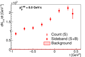
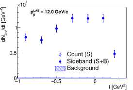
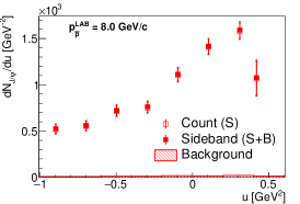
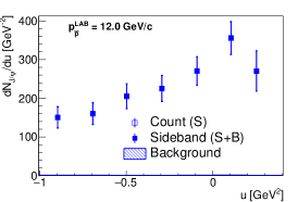
Figure 19: The count rate of fully reconstructed $J/\psi\pi^{0}$ events as a function of $t$ in the near-forward (top row) and as a function of $u$ in the near-backward (bottom row) kinematic approximation validity ranges for the three incident $\bar{p}$ momenta: 5.5 GeV/$c$ (left column), 8.0 GeV/$c$ (middle column) and 12.0 GeV/$c$ (right column). The full points are obtained using the sideband method from foreground (S+B) histograms as explained in Section V.8. The open symbols denote the count rates for signal only simulations (S) within the range 2.8 $<$ $M_{e^{+}e^{-}}$ $<$ 3.3 GeV/$c^{2}$. The amount of background within the same window is shown by the shaded histogram. The plot corresponds to an integrated luminosity of 2 fb^-1, after application of all cuts (EID, $\chi^{2}$ from kinematic fitting, number of photons per event).

V.9 Efficiency Correction

This section describes a procedure for efficiency correction of the reconstructed signal count rate to obtain differential cross sections, and compare the result to the TDA model that was used to generate the signal events. The result will also serve as a guide to the statistical uncertainties expected for this measurement. For illustration, the $t$ variable in the near-forward kinematic approximation is used, but the same arguments hold for the near-backward kinematic approximation if $t$ is replaced by $u$. The fully corrected data points at a given value of $t$ are calculated using the equation:

$$\frac{d\sigma}{dt}(t)=\frac{1}{\mathcal{L}_{int}\cdot BR(J/\psi\to e^{+}e^{-})}\frac{1}{\varepsilon(t)}\frac{N_{J/\psi\pi^{0}}(t)}{\Delta t},$$ (21)

where $\mathcal{L}_{int}$ is the integrated luminosity (2 fb^-1), and $BR(J/\psi\to e^{+}e^{-})$ indicates the branching ratio of the $J/\psi\to e^{+}e^{-}$ decay channel (5.94%). The quantity $N_{J/\psi\pi^{0}}$ is the number of reconstructed $J/\psi\pi^{0}$ events in a particular bin in $t$, and $\Delta t$ is the width of the bin. The location of the point on the $t$ axis is determined by the mean $t$ value of all the entries in the given $t$-bin at the generator level.

For the efficiency calculation, a separate simulation data set of the signal channel was used. The efficiency correction $\varepsilon(t)$ in a given bin $[t_{\min},\ t_{\max}]$ is defined as the ratio of the number of reconstructed events to the number of the generated events within that window:

$$\varepsilon(t)=\frac{N^{REC}_{J/\psi\pi^{0}}(t_{\min}<t_{REC}<t_{\max})}{N^{GEN}_{J/\psi\pi^{0}}(t_{\min}<t_{MC}<t_{\max})}.$$ (22)

We note that in the numerator, the number of signal events is counted in a bin determined by the reconstructed value of $t$, denoted by $t_{REC}$, whereas in the denominator the generated (true MC) value of $t$, denoted by $t_{MC}$, is used. The signal reconstruction efficiencies calculated in this manner for the three incident $\bar{p}$ momenta are shown in Fig. 20 for the full kinematic range accessible at each energy regardless of the validity range of the TDA model. The efficiency as a function of $u$ is just the mirror image of this distribution, where the point of reflection sits midway on the full domain covered at the particular energy. Therefore, the efficiency for the backward $\pi^{0}$ emission can be deduced from this plot by looking at the most negative values of $t$. For clarity, the validity ranges of the TDA model on the $t$ axis for both the near-forward and near-backward kinematic approximation regimes are shown as arrows at the bottom of the plot with a color that corresponds to the efficiency histogram. As far as count rates are concerned, this efficiency plot illustrates that our study, which is based on the TDA model, can be extrapolated to any other model. In particular, the reaction $\bar{p}p\to J/\psi\pi^{0}$ was recently studied in a hadronic model including intermediate baryonic resonances Van de Wiele and Ong (2013), where detailed predictions have been made for the center of mass energy dependence of the cross section and the $\pi^{0}$ angular distribution, which can be compared to the future $\overline{\mbox{\sf P}}$ANDA data. While the efficiency in the near-forward and near-backward regimes for the lowest beam momentum (5.5 GeV/$c$) are more or less comparable, this is not true for the higher beam momenta, where the efficiency in the backward regime tails off to lower values. This is due to the increasing probability for one of the leptons from the $J/\psi$ decay to fall in the forward spectrometer region outside the acceptance of the detectors included in this analysis.

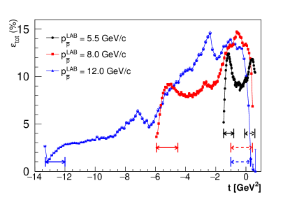
Figure 20: The overall signal reconstruction efficiency as a function of $t$ for the three incident $\bar{p}$ momenta considered in this study: 5.5 GeV/$c$ (circles), 8.0 GeV/$c$ (squares) and 12.0 GeV/$c$ (triangles). Note that the distribution as a function of $u$ is a reflection of these distributions with respect to their individual center point. The arrows span the near-forward (dashed line) and near-backward (solid line) kinematic validity ranges of the TDA model.

VI Sensitivity for Testing TDA Model

VI.1 Differential Cross Sections

Figure 21 shows a comparison between the expected precision of the measured differential cross section for an integrated luminosity of 2 fb^-1 to the prediction of Ref. Pire et al. (2013) that was used as the basis for the signal event generator. The measurements have a satisfactory precision of about 8 – 10% relative uncertainty. This level of precision will allow a quantitative test of the prediction of TDA models.

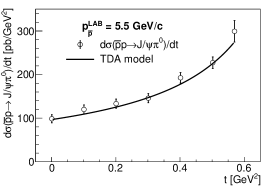
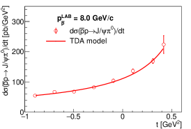
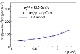
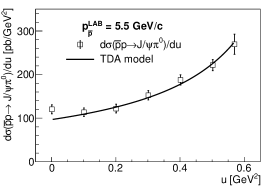
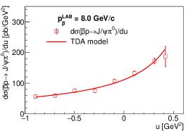
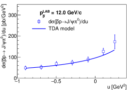
Figure 21: Comparison between the cross sections extracted from the fully efficiency corrected yields expected from 2 fb^-1 integrated luminosity (data points) and the TDA model prediction (full curves) at the three incident $\bar{p}$ momenta: 5.5 GeV/$c$ (left column), 8.0 GeV/$c$ (middle column) and 12.0 GeV/$c$ (right column). Top row: Near-forward kinematic approximation validity range as a function of $t$. Bottom row: Near-backward kinematic approximation validity range as a function of $u$.

VI.2 $J/\psi$ Decay Angular Distributions

The angular distribution of the $e^{+}$ and $e^{-}$ in the $J/\psi$ reference frame constitutes a key observable that could allow to test the validity of the factorization approach. The leading twist description of the TDA model predicts a specific form for the differential cross section with respect to the polar emission angle of the $e^{+}$ or $e^{-}$ in the $J/\psi$ reference frame relative to the direction of motion of the $J/\psi$, $\theta^{e^{+}}_{J/\psi}$:

$$\frac{d\sigma}{d\theta^{e^{+}}_{J/\psi}}\sim 1+\cos^{2}(\theta^{e^{+}}_{J/\psi}).$$ (23)

This section gives results of an attempt to reconstruct the differential angular distribution with an assumed 2 fb^-1 of integrated luminosity.

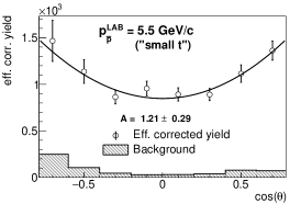
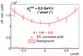
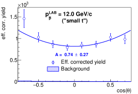
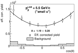
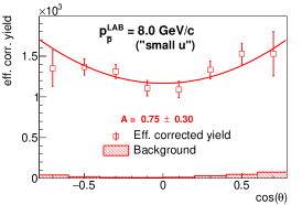
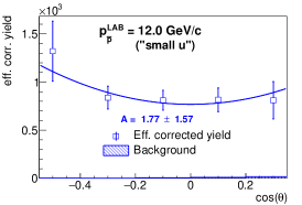
Figure 22: Efficiency corrected yield of $\bar{p}p\to J/\psi\pi^{0}\to e^{+}e^{-}\pi^{0}$ (open markers) and background yield (shaded histogram) as a function of $\cos(\theta^{e^{+}}_{J/\psi})$ and the result of the fit with the function $B\times(1+A\cos^{2}(\theta^{e^{+}}_{J/\psi}))$ (solid line) at the three incident $\bar{p}$ momenta: 5.5 GeV/$c$ (left column), 8.0 GeV/$c$ (middle column) and 12.0 GeV/$c$ (right column). Top row: Near-forward kinematic approximation validity range as a function of $t$. Bottom row: Near-backward kinematic approximation validity range as a function of $u$.

Following the same analysis procedure as the one used for the differential cross section plots of Section VI.1, the yield of signal events is extracted in bins of reconstructed $\cos(\theta^{e^{+}}_{J/\psi})$, within the small $t$ and small $u$ validity ranges separately at each energy. The yields are corrected by the efficiency as a function of $\cos(\theta^{e^{+}}_{J/\psi})$ and fitted to the functional form $B\times(1+A\cos^{2}(\theta^{e^{+}}_{J/\psi}))$. An example of the fit is shown in Fig. 22 for events weighted according to $(1+\cos^{2}(\theta^{e^{+}}_{J/\psi}))$. The statistical errors are for an assumed integrated luminosity of 2 fb^-1. There is no sensitivity to $A$ in the $u$ channel at the highest collision energy simulated due to low efficiency.

The background contamination is indicated by a shaded histogram in Fig. 22, in the same way as for Fig. 19. At the highest beam momentum, the contamination is negligible in all bins. At the lowest beam momentum, the background reaches $\approx$ 15% for some of the bins. About 60% of the background is due to the $\pi^{+}\pi^{-}\pi^{0}$ contribution, which is subtracted by the sideband analysis, as described in Section V.8. The remaining contribution is dominated by the $J/\psi\pi^{0}\pi^{0}$ and is $\lesssim$ 5% for all bins. As already mentioned, this contribution will be measured, allowing for a subtraction with a residual systematic error below 1%, which is much smaller than the statistical errors.

To estimate the expected statistical error on the measurement of parameter $A$ in a way that does not depend on the particular statistical fluctuation of the selected simulation sub-sample, the fit was repeated multiple times, each time using a different set of simulated events. The root mean square values of the distributions of these fit results is used to estimate the expected uncertainty on the measurement. We find that the extraction of the angular distribution is feasible with $\overline{\mbox{\sf P}}$ANDA with an integrated luminosity of 2 fb^-1, except in some kinematic zones where the efficiency is too low, e.g. within the backward kinematic approximation validity range of the TDA model at the largest beam momentum studied. The extraction of the parameter $A$ will be possible with errors of the order of $\approx~{}\pm$0.3 for $A=1$ and about $\approx~{}\pm$0.2 for $A=0.4$ and $A=0$. With this level of precision, it will be possible to test the leading twist approximation employed by the TDA model and potentially differentiate between models that predict angular distributions that deviate significantly from $1+\cos^{2}(\theta^{e^{+}}_{J/\psi})$.

VI.3 Systematic Uncertainties

One of the sources of systematic uncertainty is expected to come from the determination of beam luminosity. With the LMD, the uncertainty on the absolute time integrated luminosity will amount to about 5% Pan . Another source of systematic uncertainty will be associated with the signal extraction, namely from the $\pi^{+}\pi^{-}\pi^{0}$ background subtraction procedure using the sideband method, as well as from uncertainties related to the estimation of residual background from $J/\psi\pi^{0}\pi^{0}$ events, which will amount to about 1% in the pessimistic scenario assumed in this work. Finally, there will be a contribution to the systematic uncertainty coming from the calculation of the efficiency correction, but this can only be determined by how well the simulation describes the performance of the fully constructed detector. For the current study, we simulated $6\times 10^{6}$ events to calculate the efficiency at each beam momentum; as a result, the statistical uncertainty on the efficiency is negligible.

VII Conclusions

In this study, the feasibility of measuring $J/\psi\pi^{0}$ production in $\bar{p}p$ annihilation reactions with $\overline{\mbox{\sf P}}$ANDA at the future FAIR facility was investigated. The study is based on the TDA model for the description of the signal. A combination of available data and the established hadronic event generator DPM was used to describe the background with only pions in the final state. Non-resonant $J/\psi\pi^{0}\pi^{0}$ was also considered, for which a PHSP event generator was used for the event distributions and conservative estimates were made for the cross sections given the lack of constraints from existing data. Generated events were simulated and reconstructed using the PandaRoot software based on the proposed $\overline{\mbox{\sf P}}$ANDA setup.

Using events selected to include a $\pi^{0}$ and an $e^{+}e^{-}$ pair with invariant mass inside a broad window around the $J/\psi$ mass, background reactions with no $J/\psi$ in the final state can be reduced to the level of a few percent. The residual background can be subtracted using the procedure outlined. The signal efficiency decreases from 18% for beam momentum of 5.5 GeV/$c$ to 9% for 12.0 GeV/$c$. To reject the $J/\psi\pi^{0}\pi^{0}$ background reaction to the 2% level, additional selection based on kinematic fits is needed, which further reduces the signal efficiency by about an additional 30%. The severeness of these cuts will however be adjusted depending on the measured yield for this background channel.

The cross section plots were produced with the assumption of a 2 fb^-1 integrated luminosity which could be accumulated in approximately five months of data taking at each beam momentum setting with the full design luminosity of the FAIR accelerator complex. The resulting uncertainties to measure the differential cross section as a function of the four momentum transfer in the two validity regions is expected to be of the order of 5 – 10%. In addition, the angular distribution of the leptons in the $J/\psi$ center of mass frame provide important information to test the leading-twist approximation used in the TDA model. The distribution of these observables can also serve as a test of other models, as the recent hadronic model of Ref. Van de Wiele and Ong (2013), which will be particularly interesting outside the validity range of the TDA model at large emission angles.

We conclude that the measurement proposed here can be performed with $\overline{\mbox{\sf P}}$ANDA, even at c.m. energies corresponding to resonances with a forbidden or weak decay to $J/\psi\pi^{0}$. Together with $\bar{p}p\to\gamma^{*}\pi^{0}\to e^{+}e^{-}\pi^{0}$, the measurement of the $\bar{p}p\to J/\psi\pi^{0}$ reaction will enable to test TDA models and opens exciting perspectives for the study of nucleon and antinucleon structure.