Wilson loops in 3d $\mathcal{N}=4$ SQCD from Fermi gas

Abstract

We study 1/2 BPS Wilson loops in 3d $\mathcal{N}=4$ $U(N)$ Yang-Mills theory with one adjoint and $N_{f}$ fundamental hypermultiplets from the Fermi gas approach. By numerical fitting, we find the first few worldsheet instanton corrections to the Wilson loops with winding numbers 1, 2 and 3. We verify that our Fermi gas results are consistent with the matrix model results in the planar limit.

1 Introduction

Fermi gas approach MP is a powerful technique to study large $N$ behavior of the partition functions of various three dimensional theories. Of particular interest is the so called ABJ(M) theory Aharony:2008ug ; Aharony:2008gk which describes the worldvolume theory on $N$ M2-branes on the orbifold $\mathbb{C}^{4}/\mathbb{Z}_{k}$. It turns out that the partition function of ABJ(M) theory on a three sphere correctly reproduces the $N^{3/2}$ scaling of free energy expected from the holographically dual M-theory on $AdS_{4}\times S^{7}/\mathbb{Z}_{k}$ Drukker:2010nc . The Fermi gas formalism enables us to go further beyond this perturbative behavior, and now we have a complete understanding of the instanton corrections to the free energy coming from wrapped M2-branes on the bulk M-theory side (see Hatsuda:2015gca ; Marino:2016new for reviews). Also, Fermi gas formalism can be applied to the computation of Wilson loops in ABJ(M) theory and many interesting properties were uncovered in the last few years KMSS ; HHMO ; Matsumoto:2013nya ; Hatsuda:2016rmv ; Matsuno:2016jjp ; Okuyama:2016deu ; Kiyoshige:2016lno . However, for many theories with less supersymmetry than the ABJ(M) case, we are still lacking a detailed understanding of the large $N$ behavior of free energy.

In Mezei:2013gqa ; Grassi:2014vwa ; HO , some progress has been made in the so called $N_{f}$ matrix model which describes the $S^{3}$ partition function of $d=3$ $\mathcal{N}=4$ $U(N)$ Yang-Mills theory coupled to one adjoint and $N_{f}$ fundamental hypermultiplets. This theory naturally appears as the worldvolume theory of $N$ D2-branes in the presence of $N_{f}$ D6-branes, which in turn is holographically dual to M-theory on $AdS_{4}\times S^{7}/\mathbb{Z}_{N_{f}}$ in the large $N$ limit. Here the $\mathbb{Z}_{N_{f}}$ action on $S^{7}$ is induced from the orbifold $\mathbb{C}^{2}\times(\mathbb{C}^{2}/\mathbb{Z}_{N_{f}})$ with $A_{N_{f}-1}$ ALE singularity. By the 3d $\mathcal{N}=4$ mirror symmetry, this theory is dual to a $\widehat{A}_{N_{f}-1}$ quiver gauge theory Intriligator:1996ex ; deBoer:1996mp . As emphasized in Grassi:2014vwa , the $N_{f}$ matrix model admits not only the ordinary ’t Hooft limit (type IIA limit on the bulk side)

$$N,N_{f}\to\infty\quad\text{with}~{}~{}\lambda=\frac{N}{N_{f}}:~{}\text{fixed},$$ (1)

but also the M-theory limit

$$N\to\infty\quad\text{with}~{}~{}N_{f}:~{}\text{fixed}.$$ (2)

Here $1/N_{f}$ plays the role of string coupling. An important consequence of the Fermi gas description is that these two limits are actually smoothly connected since the grand partition function of $N_{f}$ matrix model is a completely well defined quantity for any value of $N_{f}$. In HO , the first few instanton corrections to the grand potential were determined in a closed form as a function of $N_{f}$; it is found that the structure of instanton corrections of $N_{f}$ matrix model is quite different from the ABJM case, and in particular there is no obvious connection with the topological string. However, the pole cancellation mechanism between worldsheet instantons and membrane instantons, originally found in the ABJM case Hatsuda:2012dt , works also in the $N_{f}$ matrix model HO .

In this paper, we will consider the Wilson loops in the $N_{f}$ matrix model from the Fermi gas approach. We will focus on the 1/2 BPS Wilson loop on $S^{3}$ which wraps $m$ times around the equator. By the numerical fitting, we find the first few worldsheet instanton corrections to the vacuum expectation value (VEV) of winding Wilson loops with winding number $m=1,2,3$. We find that our Fermi gas result is consistent with the planar VEV of winding Wilson loops in the ’t Hooft limit (1) obtained from the resolvent of $N_{f}$ matrix model Grassi:2014vwa . Our Fermi gas result suggests that there is no “pure” membrane instanton corrections to the Wilson loop VEVs except for the contributions from bound states of membrane instantons and worldsheet instantons. This is reminiscent of the instanton corrections to the 1/2 BPS Wilson loops in ABJ(M) theory HHMO ; Hatsuda:2016rmv .

This paper is organized as follows. In section 2, we consider VEVs of 1/2 BPS winding Wilson loops in $N_{f}$ matrix model from the Fermi gas approach and explain our numerical method to compute them. In section 3, we find the perturbative part of winding Wilson loops in a closed from, and in section 4 we determine the first few worldsheet instanton corrections for the Wilson loops with winding number $m=1,2,3$. In section 5, we reproduce the perturbative part of Wilson loop in the fundamental representation from the WKB expansion of spectral traces. In section 6, we summarize the planar solution of $N_{f}$ matrix model obtained in Grassi:2014vwa . We find that the planar resolvent in Grassi:2014vwa can be vastly simplified. In section 7, we compare the Fermi gas results and the matrix model results of the Wilson loop VEVs in the planar limit and find a perfect agreement. Finally, we conclude in section 8. In appendix A we list some exact values of Wilson loop VEVs and in appendix B we mention some curious properties of Wilson loops for $N_{f}=4$.

2 Winding Wilson loops

2.1 Review of $N_{f}$ matrix model

First we review the $S^{3}$ partition function of $d=3$ $\mathcal{N}=4$ $U(N)$ Yang-Mills theory with one adjoint and $N_{f}$ fundamental hypermultiplets. In $d=3$, the gauge coupling has mass dimension $1/2$ and it flows to infinity in the IR. Thus the gauge kinetic term is irrelevant in IR and the $S^{3}$ partition function of this theory is independent of the gauge coupling. This theory flows to a superconformal fixed point in the IR, which is conjectured to be holographically dual to M-theory on $AdS_{4}\times S^{7}/\mathbb{Z}_{N_{f}}$.

Using the supersymmetric localization, the $S^{3}$ partition function is reduced to a finite dimensional integral Kapustin:2009kz , which is dubbed the $N_{f}$ matrix model in Grassi:2014vwa

$$\begin{aligned} Z(N,N_{f})&=\frac{1}{N!}\int\frac{d^{N}x}{(4\pi)^{N}}\prod_{i=1}^{N}\frac{1}{(2\cosh\frac{x_{i}}{2})^{N_{f}}}\prod_{i<j}\tanh^{2}\frac{x_{i}-x_{j}}{2}.\end{aligned}$$ (3)

Using the Cauchy identity, (3) can be rewritten as a partition function of $N$ fermions on a real line

$$Z(N,N_{f})=\frac{1}{N!}\int d^{N}x\sum_{\sigma\in S_{N}}(-1)^{\sigma}\prod_{i=1}^{N}\rho(x_{i},x_{\sigma(i)})$$ (4)

where the density matrix $\rho$ is given by

$$\rho(x,y)=\frac{1}{2\pi}\frac{1}{(2\cosh\frac{x}{2})^{N_{f}/2}}\frac{1}{2\cosh\frac{x-y}{2}}\frac{1}{(2\cosh\frac{y}{2})^{N_{f}/2}}.$$ (5)

It is also useful to express $\rho(x,y)$ as a matrix element of the quantum mechanical operator $\widehat{\rho}$

$$\begin{aligned} \rho(x,y)=\langle x|\widehat{\rho}|y\rangle,\qquad\widehat{\rho}=\frac{1}{(2\cosh\frac{\widehat{x}}{2})^{N_{f}/2}}\frac{1}{2\cosh\frac{\widehat{p}}{2}}\frac{1}{(2\cosh\frac{\widehat{x}}{2})^{N_{f}/2}},\end{aligned}$$ (6)

with $\widehat{x}$ and $\widehat{p}$ being the coordinate and momentum of a fermion obeying the canonical commutation relation

$$[\widehat{x},\widehat{p}]={\rm i}\hbar,\qquad\hbar=2\pi.$$ (7)

As discussed in MP , it is more convenient to consider the grand canonical ensemble by summing over $N$ with fugacity $\kappa=e^{\mu}$. It turns out that the grand partition function is written as a Fredholm determinant

$$\Xi(\mu,N_{f})=1+\sum_{N=1}^{\infty}\kappa^{N}Z(N,N_{f})=\operatorname{Det}(1+\kappa\rho)$$ (8)

which in turn is physically interpreted as a grand canonical ensemble of ideal Fermi gas MP . The large $N$ behavior of canonical partition function $Z(N,N_{f})$ can be deduced from the large $\mu$ behavior of the modified grand potential $J(\mu,N_{f})$, which is related to the grand partition function by Hatsuda:2012dt

$$\Xi(\mu,N_{f})=\sum_{n\in\mathbb{Z}}e^{J(\mu+2\pi{\rm i}n,N_{f})}.$$ (9)

Then the canonical partition function is recovered from $J(\mu,N_{f})$ by the integral transformation

$$Z(N,N_{f})=\int_{\mathcal{C}}\frac{d\mu}{2\pi{\rm i}}e^{J(\mu,N_{f})-N\mu}$$ (10)

where $\mathcal{C}$ is a contour on the $\mu$-plane running from $e^{\frac{\pi{\rm i}}{3}}\infty$ to $e^{-\frac{\pi{\rm i}}{3}}\infty$.

The modified grand potential $J(\mu,N_{f})$ can be decomposed into several pieces:

$$J(\mu,N_{f})=J^{\text{pert}}(\mu,N_{f})+J^{\text{WS}}(\mu,N_{f})+J^{\text{M2}}(\mu,N_{f})+J^{\text{bound}}(\mu,N_{f})$$ (11)

The first term of (11) is the perturbative part

$$J^{\text{pert}}(\mu,N_{f})=\frac{C\mu^{3}}{3}+B\mu+A,$$ (12)

where $C,B,$ and $A$ are given by Mezei:2013gqa ; Grassi:2014vwa ; HO

$$\begin{aligned} C=\frac{2}{N_{f}\pi^{2}},\qquad B=\frac{1}{2N_{f}}-\frac{N_{f}}{8},\qquad A=\frac{1}{2}A_{c}(N_{f})+\frac{1}{2}A_{c}(1)N_{f}^{2}.\end{aligned}$$ (13)

Here $A_{c}(N_{f})$ is a certain resummation of the constant map contributions of topological string Hanada:2012si ; Hatsuda:2015owa ; HO

$$A_{c}(N_{f})=-\frac{N_{f}^{2}\zeta(3)}{8\pi^{2}}+4\int_{0}^{\infty}dx\frac{x}{e^{x}-1}\log\Bigl{(}2\sinh\frac{2\pi x}{N_{f}}\Bigr{)}.$$ (14)

As shown in HO , $A_{c}(N_{f})$ can be evaluated in a closed form for integer $N_{f}$. In particular, for $N_{f}=1$ we find

$$A_{c}(1)=-\frac{\zeta(3)}{8\pi^{2}}+\frac{1}{4}\log 2.$$ (15)

$J^{\text{WS}}(\mu,N_{f})$ and $J^{\text{M2}}(\mu,N_{f})$ in (11) denote the worldsheet instanton and membrane instanton corrections, respectively, while the last term $J^{\text{bound}}(\mu,N_{f})$ in (11) represents the contributions from the bound states of worldsheet instantons and membrane instantons. In HO , the first few instanton corrections are determined: the worldsheet instantons are given by

$$\begin{aligned} J^{\text{WS}}(\mu,N_{f})&=-\frac{4\mu+N_{f}}{2\pi\sin\frac{2\pi}{N_{f}}}e^{-\frac{4\mu}{N_{f}}}\\ &+\left[-\frac{(4\mu+N_{f})^{2}}{4\pi^{2}}+\frac{3\sin\frac{6\pi}{N_{f}}(8\mu+N_{f})}{8\pi\sin\frac{2\pi}{N_{f}}\sin\frac{4\pi}{N_{f}}}-\frac{\sin\frac{8\pi}{N_{f}}}{2\sin^{2}\frac{2\pi}{N_{f}}\sin\frac{4\pi}{N_{f}}}\right]e^{-\frac{8\mu}{N_{f}}}+\mathcal{O}(e^{-\frac{12\mu}{N_{f}}})\end{aligned}$$ (16)

and the membrane 1-instanton is given by

$$J^{\text{M2}}(\mu,N_{f})=-\frac{\Gamma\bigl{(}-\frac{N_{f}}{2}\bigr{)}^{2}}{4\pi^{2}\Gamma(-N_{f})}(2\mu+1)e^{-2\mu}+\mathcal{O}(e^{-4\mu}).$$ (17)

At present, we do not know the exact form of the bound states in the $N_{f}$ matrix model.

In the large $N$ limit, the integral (10) can be evaluated by the saddle point approximation, where the saddle point value $\mu_{*}$ of the chemical potential is given by

$$\mu_{*}\approx\sqrt{\frac{N}{C}}=\pi\sqrt{\frac{NN_{f}}{2}}.$$ (18)

Plugging this value $\mu_{*}$ into the perturbative part of grand potential, we recover the $N^{3/2}$ behavior of free energy

$$-\log Z(N,N_{f})\approx N\mu_{*}-J^{\text{pert}}(\mu_{*},N_{f})\approx\frac{\pi\sqrt{2N_{f}}}{3}N^{3/2}.$$ (19)

Also, the free energy receives instanton corrections of order

worldsheet 1-instanton $$:~{}e^{-\frac{4\mu_{*}}{N_{f}}}=e^{-2\pi\sqrt{2N/N_{f}}},$$ (20)

membrane 1-instanton $$:~{}e^{-2\mu_{*}}=e^{-2\pi\sqrt{N_{f}N/2}}.$$ (21)

2.2 Wilson loops in $N_{f}$ matrix model

In this paper, we will study the VEV of 1/2 BPS Wilson loops in the $N_{f}$ matrix model. The 1/2 BPS Wilson loop in representation $R$ is given by Assel:2015oxa

$$\operatorname{Tr}_{R}\mathcal{P}\exp\left[\oint ds\bigl{(}A_{\mu}\dot{x}^{\mu}+\sigma|\dot{x}|\bigr{)}\right]$$ (22)

where $\sigma$ is one of the three scalar fields in the $\mathcal{N}=4$ vectormultiplet and $x^{\mu}(s)$ parametrizes the equator of $S^{3}$. The VEV of such BPS Wilson loops can be reduced to a finite dimensional integral by the supersymmetric localization Kapustin:2009kz . Here we will focus on the Wilson loop wound around the equator of $S^{3}$ $m$ times, which we will call the winding Wilson loop with winding number $m$.

Now, let us consider the (un-normalized) VEV of winding Wilson loop

$$W_{m}(N,N_{f})=\Biggl{\langle}\sum_{i=1}^{N}e^{mx_{i}}\Biggr{\rangle}$$ (24)

where the expectation value is defined by

$$\langle\mathcal{O}\rangle=\frac{1}{N!}\int\frac{d^{N}x}{(4\pi)^{N}}\,\mathcal{O}\prod_{i=1}^{N}\frac{1}{(2\cosh\frac{x_{i}}{2})^{N_{f}}}\prod_{i<j}\tanh^{2}\frac{x_{i}-x_{j}}{2}.$$ (25)

Note that the integral defining $W_{m}(N,N_{f})$ is convergent if $N_{f}$ satisfies the condition

$$N_{f}>2m.$$ (26)

As in the case of ABJM theory KMSS ; HHMO , we can study the Wilson loop VEV of $N_{f}$ matrix model from the Fermi gas approach. As discussed in HHMO , using the relation

$$\sum_{N=0}^{\infty}\kappa^{N}\Biggl{\langle}\prod_{i=1}^{N}(1+\varepsilon e^{mx_{i}})\Biggr{\rangle}=\text{Det}\Bigl{(}1+\kappa\rho(1+\varepsilon e^{mx})\Bigr{)}$$ (27)

and picking up the $\mathcal{O}(\varepsilon)$ term on both sides, we find that the grand canonical VEV of winding Wilson loop is written as

$$\begin{aligned} W_{m}(\mu,N_{f})=\sum_{N=1}^{\infty}\kappa^{N}W_{m}(N,N_{f})=\mathrm{Det}(1+\kappa\rho)\operatorname{Tr}\left(\frac{\kappa\rho}{1+\kappa\rho}e^{mx}\right).\end{aligned}$$ (28)

In the following, we will mainly consider the grand canonical VEV of winding Wilson loops normalized by the grand partition function

$$\frac{W_{m}(\mu,N_{f})}{\Xi(\mu,N_{f})}=\operatorname{Tr}\left(\frac{\kappa\rho}{1+\kappa\rho}e^{mx}\right).$$ (29)

2.3 Computation of trace

To compute the grand canonical VEV of Wilson loop (29), we have to evaluate the trace $\operatorname{Tr}(\rho^{\ell}e^{mx})$

$$\frac{W_{m}(\mu,N_{f})}{\Xi(\mu,N_{f})}=\sum_{\ell=1}^{\infty}(-1)^{\ell-1}\kappa^{\ell}\operatorname{Tr}(\rho^{\ell}e^{mx}).$$ (30)

This can be done systematically using the Tracy-Widom lemma TW . Noticing that $\rho$ is written as

$$\begin{aligned} \rho(x,y)&=\frac{E(x)E(y)}{M(x)+M(y)},\\ M(x)=e^{x}&,\qquad E(x)=\sqrt{\frac{1}{2\pi}\frac{e^{x}}{(2\cosh\frac{x}{2})^{N_{f}}}},\end{aligned}$$ (31)

one can show the $\ell^{\text{th}}$ power of $\rho$ is given by TW

$$\rho^{\ell}(x,y)=\frac{E(x)E(y)}{M(x)+(-1)^{\ell-1}M(y)}\sum_{j=0}^{\ell-1}(-1)^{j}\psi_{j}(x)\psi_{\ell-1-j}(y),$$ (32)

where the functions $\psi_{j}(x)~{}(j=0,1,\cdots)$ are determined recursively starting from $\psi_{0}(x)=1$

$$\begin{aligned} \psi_{j}(x)&=\frac{1}{E(x)}\int dy\rho(x,y)E(y)\psi_{j-1}(y).\end{aligned}$$ (33)

When $N_{f}$ is an integer, one can compute the exact values of VEV by closing the contour and picking up the residue of poles, as in the case of ABJM theory Okuyama:2011su ; Hatsuda:2012hm ; Putrov:2012zi ; Hatsuda:2012dt . In appendix A, we list some examples of the exact values of Wilson loop VEVs.

As explained in Okuyama:2016deu , we can also compute the sequence of functions $\{\psi_{j}\}$ numerically with high precision by discrete Fourier transformations.

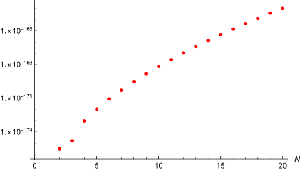
Figure 1: Plot of the numerical error $e_{N}$ (34) of the fundamental Wilson loop for $N_{f}=6$.

We can estimate the accuracy of our numerics by comparing with the exact values in appendix A. As an example, let us consider the Wilson loop VEV in the fundamental representation (or winding number $m=1$) for $N_{f}=6$. We have computed the exact values of $W_{\vbox{\offinterlineskip\kern 1.0pt\hbox{\kern 1.0pt\vbox{\hbox{\noindent\vbox{\hbox{\vbox to0.0pt{\hrule height=0.4pt,width=3.90555pt\vss}}\hbox{\vbox{\hbox to0.0pt{\vrule width=0.4pt,height=3.90555pt\hss}}\kern 3.90555pt\vbox{\hbox to0.0pt{\vrule width=0.4pt,height=3.90555pt\hss}}}\hbox{\vbox{\hbox{\vbox to0.0pt{\hrule height=0.4pt,width=4.30554pt\vss}}}\kern-0.4pt}}}\hbox{} }\kern 1.0pt\kern 0.4pt}\kern 1.0pt\kern 0.4pt}}(N,N_{f}=6)$ up to $N=20$, and in Fig. 1 we plotted the relative error

$$e_{N}=\left|\frac{W_{\vbox{\offinterlineskip\kern 1.0pt\hbox{\kern 1.0pt\vbox{\hbox{\noindent\vbox{\hbox{\vbox to0.0pt{\hrule height=0.4pt,width=3.90555pt\vss}}\hbox{\vbox{\hbox to0.0pt{\vrule width=0.4pt,height=3.90555pt\hss}}\kern 3.90555pt\vbox{\hbox to0.0pt{\vrule width=0.4pt,height=3.90555pt\hss}}}\hbox{\vbox{\hbox{\vbox to0.0pt{\hrule height=0.4pt,width=4.30554pt\vss}}}\kern-0.4pt}}}\hbox{} }\kern 1.0pt\kern 0.4pt}\kern 1.0pt\kern 0.4pt}}(N,6)_{\text{numerical}}}{W_{\vbox{\offinterlineskip\kern 1.0pt\hbox{\kern 1.0pt\vbox{\hbox{\noindent\vbox{\hbox{\vbox to0.0pt{\hrule height=0.4pt,width=3.90555pt\vss}}\hbox{\vbox{\hbox to0.0pt{\vrule width=0.4pt,height=3.90555pt\hss}}\kern 3.90555pt\vbox{\hbox to0.0pt{\vrule width=0.4pt,height=3.90555pt\hss}}}\hbox{\vbox{\hbox{\vbox to0.0pt{\hrule height=0.4pt,width=4.30554pt\vss}}}\kern-0.4pt}}}\hbox{} }\kern 1.0pt\kern 0.4pt}\kern 1.0pt\kern 0.4pt}}(N,6)_{\text{exact}}}-1\right|,$$ (34)

between the exact and the numerical values. As we can see from Fig. 1, our numerics has a high precision with an extremely small error

$$e_{N}<1.1\times 10^{-163}\quad(\text{for}~{}~{}N\leq 20).$$ (35)

On the other hand, the instanton factors (21) for $N_{f}=6,N=20,$ are given by

$$\begin{aligned} \text{worldsheet~{}1-instanton}&:~{}e^{-2\pi\sqrt{2N/N_{f}}}\approx 9.0\times 10^{-8},\\ \text{membrane~{}1-instanton}&:~{}e^{-2\pi\sqrt{N_{f}N/2}}\approx 7.3\times 10^{-22}.\end{aligned}$$ (36)

From (35) and (36), one can see that our numerical computation has enough accuracy to study instanton corrections to the Wilson loop VEVs. Also, from (36) we observe that the membrane instanton correction is highly suppressed compared to the worldsheet instanton correction. This is a generic phenomenon in the convergence region (26). Thus it is difficult to study membrane instanton corrections to the Wilson loops numerically; in this paper we will mainly consider the worldsheet instanton corrections to the Wilson loop VEVs.

2.3.1 Odd winding number

It turns out that the grand canonical VEV in (29) for odd $m$ can be rewritten in a simpler form. Let us first consider the fundamental representation. We notice that Wilson loop factor $e^{mx}$ for $m=1$ reduces to $M(x)$ in (31). Then the trace $\operatorname{Tr}(\rho^{\ell}M)$ can be simplified using the formal operator relation

$$M\rho+\rho M=|E\rangle\langle E|.$$ (37)

Then we have

$$\begin{aligned} \operatorname{Tr}(\rho^{\ell}M)=\operatorname{Tr}(\rho^{\ell-1}\rho M)=\operatorname{Tr}(\rho^{\ell-1}|E\rangle\langle E|)-\operatorname{Tr}(\rho^{\ell-1}M\rho).\end{aligned}$$ (38)

Using the cyclicity of trace, we find

$$\operatorname{Tr}(\rho^{\ell}M)=\frac{1}{2}\langle E|\rho^{\ell-1}|E\rangle.$$ (39)

Finally, we find that the grand canonical VEV of fundamental Wilson loop is written as

$$\frac{W_{\vbox{\offinterlineskip\kern 1.0pt\hbox{\kern 1.0pt\vbox{\hbox{\noindent\vbox{\hbox{\vbox to0.0pt{\hrule height=0.4pt,width=3.90555pt\vss}}\hbox{\vbox{\hbox to0.0pt{\vrule width=0.4pt,height=3.90555pt\hss}}\kern 3.90555pt\vbox{\hbox to0.0pt{\vrule width=0.4pt,height=3.90555pt\hss}}}\hbox{\vbox{\hbox{\vbox to0.0pt{\hrule height=0.4pt,width=4.30554pt\vss}}}\kern-0.4pt}}}\hbox{} }\kern 1.0pt\kern 0.4pt}\kern 1.0pt\kern 0.4pt}}(\mu,N_{f})}{\Xi(\mu,N_{f})}=\operatorname{Tr}\left(\frac{\kappa\rho}{1+\kappa\rho}M\right)=\frac{1}{2}\langle E|\frac{\kappa}{1+\kappa\rho}|E\rangle.$$ (40)

This is reminiscent of the grand canonical VEV of 1/2 BPS Wilson loops in ABJM theory HHMO . More generally, for odd $m$ one can show that

$$\frac{W_{m}(\mu,N_{f})}{\Xi(\mu,N_{f})}=\operatorname{Tr}\left(\frac{\kappa\rho}{1+\kappa\rho}M^{m}\right)=\frac{1}{2}\sum_{j=0}^{m-1}(-1)^{j}\langle E|M^{j}\frac{\kappa}{1+\kappa\rho}M^{m-1-j}|E\rangle,$$ (41)

in a similar manner as (38). On the other hand, we could not find a similar expression for even winding numbers.

3 Perturbative part

In this section, we consider the large $\mu$ expansion of the grand canonical VEV (29) of winding Wilson loops. It is useful to introduce the modified version of the grand canonical VEV $\widehat{W}_{m}(\mu,N_{f})$ by

$$W_{m}(\mu,N_{f})=\sum_{n\in\mathbb{Z}}e^{J(\mu+2\pi{\rm i}n,N_{f})}\widehat{W}_{m}(\mu+2\pi{\rm i}n,N_{f}).$$ (42)

As in the case of modified grand potential, $\widehat{W}_{m}(\mu,N_{f})$ is written as a sum of perturbative part and the exponentially suppressed instanton corrections.

We find that the leading term (perturbative part) of $\widehat{W}_{m}(\mu,N_{f})$ in the large $\mu$ limit is given by

$$\widehat{W}_{m}^{\text{pert}}(\mu,N_{f})=c_{m}(N_{f})e^{\frac{2m\mu}{N_{f}}}.$$ (43)

The coefficient $c_{m}(N_{f})$ in (43) can be determined as follows. As in the case of partition function (10), the canonical picture and the grand canonical picture of Wilson loop VEV are related by the integral transformation

$$W_{m}(N,N_{f})=\int_{\mathcal{C}}\frac{d\mu}{2\pi{\rm i}}e^{J(\mu,N_{f})}\widehat{W}_{m}(\mu,N_{f}).$$ (44)

Then expanding the integrand of (44)

$$e^{J(\mu,N_{f})}\widehat{W}_{m}(\mu,N_{f})=e^{J^{\text{pert}}(\mu,N_{f})+\frac{2m\mu}{N_{f}}}\sum_{j,w}a_{j,w}\mu^{j}e^{-w\mu},$$ (45)

the canonical VEV is written as a sum of Airy function and its derivatives

$$W_{m}(N,N_{f})=e^{A}C^{-\frac{1}{3}}\sum_{j,w}a_{j,w}(-\partial_{N})^{j}\text{Ai}\Biggl{[}C^{-\frac{1}{3}}\Bigl{(}N-B-\frac{2m}{N_{f}}+w\Bigr{)}\Biggr{]}.$$ (46)

In particular, the perturbative part of canonical VEV is given by

$$W_{m}^{\text{pert}}(N,N_{f})=c_{m}(N_{f})e^{A}C^{-\frac{1}{3}}\text{Ai}\Biggl{[}C^{-\frac{1}{3}}\Bigl{(}N-B-\frac{2m}{N_{f}}\Bigr{)}\Biggr{]}.$$ (47)

By fitting the numerical value of $W_{m}(N,N_{f})$ with the expression (47), we can determine the coefficient $c_{m}(N_{f})$. In this way, we find that the coefficient in the perturbative part of $\widehat{W}_{m}(\mu,N_{f})$ in (43) is given by

$$\begin{aligned} c_{1}(N_{f})&=\frac{1}{4\sin\frac{2\pi}{N_{f}}},\quad&c_{3}(N_{f})&=\frac{\sin^{2}\frac{\pi}{N_{f}}}{4\sin\frac{2\pi}{N_{f}}\sin\frac{4\pi}{N_{f}}\sin\frac{6\pi}{N_{f}}},\\ c_{2}(N_{f})&=\frac{1}{2N_{f}\sin\frac{2\pi}{N_{f}}\sin\frac{4\pi}{N_{f}}},\quad&c_{4}(N_{f})&=\frac{\sin^{2}\frac{2\pi}{N_{f}}}{2N_{f}\sin\frac{2\pi}{N_{f}}\sin\frac{4\pi}{N_{f}}\sin\frac{6\pi}{N_{f}}\sin\frac{8\pi}{N_{f}}},\end{aligned}$$ (48)

for winding numbers $m=1,\cdots,4$. For general winding number $m$, we conjecture

$$c_{m}(N_{f})=\left\{\begin{aligned} &\frac{\prod_{j=1}^{\frac{m-1}{2}}\sin^{2}\frac{(2j-1)\pi}{N_{f}}}{4\prod_{n=1}^{m}\sin\frac{2\pi n}{N_{f}}}&\quad&(\text{odd}~{}m),\\ &\frac{\prod_{j=1}^{\frac{m}{2}-1}\sin^{2}\frac{2j\pi}{N_{f}}}{2N_{f}\prod_{n=1}^{m}\sin\frac{2\pi n}{N_{f}}}&\quad&(\text{even}~{}m).\end{aligned}\right.$$ (49)

We have checked this behavior numerically for $m=1,\cdots,8$. In Fig. 2, we show the plot of Wilson loop VEV with $m=2$ as an example. As we can see from Fig. 2, the Airy function in (47) exhibits a nice agreement with the numerical value of $W_{2}(N,N_{f})$, if we use the correct coefficient $c_{2}(N_{f})$ in (48). We have also confirmed a similar agreement between $W_{m}(N,N_{f})$ and the Airy function (47) for $m=1,\cdots,8$ with the coefficient $c_{m}(N_{f})$ in (49).

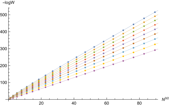
Figure 2: We show the plot of $-\log W_{2}(N,N_{f})$ for $N_{f}=5,6,\cdots,13$. Note that the horizontal axis is $N^{3/2}$, and $N_{f}$ increases from the bottom curve $(N_{f}=5)$ to the top curve $(N_{f}=13)$. The dots are the numerical values of the Wilson loop VEV while the solid curves represent the perturbative part given by the Airy function (47).

4 Instanton corrections

We can continue the numerical fitting beyond the perturbative part and fix the instanton coefficients in the expansion (45) and (46). As we will see below, we determine the first few worldsheet instanton corrections to $\widehat{W}_{m}(\mu,N_{f})$ for $m=1,2,3$ in a closed form as a function of $N_{f}$. We conjecture that there is no “pure” membrane instanton corrections to $\widehat{W}_{m}(\mu,N_{f})$ except for the contributions of bound states.

4.1 Fundamental representation

Let us first consider the fundamental representation. We find that the worldsheet instanton corrections are given by

$$\begin{aligned} \widehat{W}_{\vbox{\offinterlineskip\kern 1.0pt\hbox{\kern 1.0pt\vbox{\hbox{\noindent\vbox{\hbox{\vbox to0.0pt{\hrule height=0.4pt,width=3.90555pt\vss}}\hbox{\vbox{\hbox to0.0pt{\vrule width=0.4pt,height=3.90555pt\hss}}\kern 3.90555pt\vbox{\hbox to0.0pt{\vrule width=0.4pt,height=3.90555pt\hss}}}\hbox{\vbox{\hbox{\vbox to0.0pt{\hrule height=0.4pt,width=4.30554pt\vss}}}\kern-0.4pt}}}\hbox{} }\kern 1.0pt\kern 0.4pt}\kern 1.0pt\kern 0.4pt}}(\mu,N_{f})&=-\frac{N_{f}}{4}+e^{\frac{2\mu}{N_{f}}}\Biggl{[}\frac{1}{4\sin\frac{2\pi}{N_{f}}}+\frac{4\mu+N_{f}}{4\pi}e^{-\frac{4\mu}{N_{f}}}\\ &+\Biggl{(}\frac{\sin\frac{2\pi}{N_{f}}(4\mu+N_{f})^{2}}{8\pi^{2}}-\frac{3\cos\frac{2\pi}{N_{f}}(8\mu+N_{f})}{8\pi}+\frac{\cos^{2}\frac{2\pi}{N_{f}}}{\sin\frac{2\pi}{N_{f}}}\Biggr{)}e^{-\frac{8\mu}{N_{f}}}\\ &+\Biggl{(}\frac{(\sin^{2}\frac{2\pi}{N_{f}}+\sin^{2}\frac{4\pi}{N_{f}})(4\mu+N_{f})^{3}}{24\pi^{3}}-\frac{3\sin\frac{4\pi}{N_{f}}\sin\frac{6\pi}{N_{f}}}{\sin\frac{2\pi}{N_{f}}}\frac{(4\mu+N_{f})(8\mu+N_{f})}{16\pi^{2}}\\ &\qquad+\frac{5\cos\frac{4\pi}{N_{f}}\sin\frac{6\pi}{N_{f}}}{9\sin\frac{2\pi}{N_{f}}}\frac{12\mu+N_{f}}{\pi}+(\cos^{2}\frac{2\pi}{N_{f}}+\cos^{2}\frac{4\pi}{N_{f}})\frac{4\mu+N_{f}}{\pi}\\ &\qquad-\frac{2(\sin\frac{6\pi}{N_{f}}+\cos\frac{6\pi}{N_{f}}\sin\frac{8\pi}{N_{f}})}{\sin\frac{2\pi}{N_{f}}\sin\frac{4\pi}{N_{f}}}\Biggr{)}e^{-\frac{12\mu}{N_{f}}}+\mathcal{O}\Bigl{(}e^{-\frac{16\mu}{N_{f}}}\Bigr{)}\Biggr{]}.\end{aligned}$$ (50)

In Fig. 3 we plot the quantity

$$\delta=\frac{W_{\vbox{\offinterlineskip\kern 1.0pt\hbox{\kern 1.0pt\vbox{\hbox{\noindent\vbox{\hbox{\vbox to0.0pt{\hrule height=0.4pt,width=3.90555pt\vss}}\hbox{\vbox{\hbox to0.0pt{\vrule width=0.4pt,height=3.90555pt\hss}}\kern 3.90555pt\vbox{\hbox to0.0pt{\vrule width=0.4pt,height=3.90555pt\hss}}}\hbox{\vbox{\hbox{\vbox to0.0pt{\hrule height=0.4pt,width=4.30554pt\vss}}}\kern-0.4pt}}}\hbox{} }\kern 1.0pt\kern 0.4pt}\kern 1.0pt\kern 0.4pt}}(N,N_{f})-W_{\vbox{\offinterlineskip\kern 1.0pt\hbox{\kern 1.0pt\vbox{\hbox{\noindent\vbox{\hbox{\vbox to0.0pt{\hrule height=0.4pt,width=3.90555pt\vss}}\hbox{\vbox{\hbox to0.0pt{\vrule width=0.4pt,height=3.90555pt\hss}}\kern 3.90555pt\vbox{\hbox to0.0pt{\vrule width=0.4pt,height=3.90555pt\hss}}}\hbox{\vbox{\hbox{\vbox to0.0pt{\hrule height=0.4pt,width=4.30554pt\vss}}}\kern-0.4pt}}}\hbox{} }\kern 1.0pt\kern 0.4pt}\kern 1.0pt\kern 0.4pt}}^{\text{pert}}(N,N_{f})-W_{\vbox{\offinterlineskip\kern 1.0pt\hbox{\kern 1.0pt\vbox{\hbox{\noindent\vbox{\hbox{\vbox to0.0pt{\hrule height=0.4pt,width=3.90555pt\vss}}\hbox{\vbox{\hbox to0.0pt{\vrule width=0.4pt,height=3.90555pt\hss}}\kern 3.90555pt\vbox{\hbox to0.0pt{\vrule width=0.4pt,height=3.90555pt\hss}}}\hbox{\vbox{\hbox{\vbox to0.0pt{\hrule height=0.4pt,width=4.30554pt\vss}}}\kern-0.4pt}}}\hbox{} }\kern 1.0pt\kern 0.4pt}\kern 1.0pt\kern 0.4pt}}^{\text{inst}}(N,N_{f})}{W_{\vbox{\offinterlineskip\kern 1.0pt\hbox{\kern 1.0pt\vbox{\hbox{\noindent\vbox{\hbox{\vbox to0.0pt{\hrule height=0.4pt,width=3.90555pt\vss}}\hbox{\vbox{\hbox to0.0pt{\vrule width=0.4pt,height=3.90555pt\hss}}\kern 3.90555pt\vbox{\hbox to0.0pt{\vrule width=0.4pt,height=3.90555pt\hss}}}\hbox{\vbox{\hbox{\vbox to0.0pt{\hrule height=0.4pt,width=4.30554pt\vss}}}\kern-0.4pt}}}\hbox{} }\kern 1.0pt\kern 0.4pt}\kern 1.0pt\kern 0.4pt}}^{\text{pert}}(N,N_{f})}e^{\frac{12\mu_{*}}{N_{f}}}$$ (51)

where $W_{\vbox{\offinterlineskip\kern 1.0pt\hbox{\kern 1.0pt\vbox{\hbox{\noindent\vbox{\hbox{\vbox to0.0pt{\hrule height=0.4pt,width=3.90555pt\vss}}\hbox{\vbox{\hbox to0.0pt{\vrule width=0.4pt,height=3.90555pt\hss}}\kern 3.90555pt\vbox{\hbox to0.0pt{\vrule width=0.4pt,height=3.90555pt\hss}}}\hbox{\vbox{\hbox{\vbox to0.0pt{\hrule height=0.4pt,width=4.30554pt\vss}}}\kern-0.4pt}}}\hbox{} }\kern 1.0pt\kern 0.4pt}\kern 1.0pt\kern 0.4pt}}^{\text{pert}}(N,N_{f})$ in (51) is the perturbative part given by the Airy function (47) and $\mu_{*}$ is the saddle point value of the chemical potential in (18), and $W_{\vbox{\offinterlineskip\kern 1.0pt\hbox{\kern 1.0pt\vbox{\hbox{\noindent\vbox{\hbox{\vbox to0.0pt{\hrule height=0.4pt,width=3.90555pt\vss}}\hbox{\vbox{\hbox to0.0pt{\vrule width=0.4pt,height=3.90555pt\hss}}\kern 3.90555pt\vbox{\hbox to0.0pt{\vrule width=0.4pt,height=3.90555pt\hss}}}\hbox{\vbox{\hbox{\vbox to0.0pt{\hrule height=0.4pt,width=4.30554pt\vss}}}\kern-0.4pt}}}\hbox{} }\kern 1.0pt\kern 0.4pt}\kern 1.0pt\kern 0.4pt}}^{\text{inst}}(N,N_{f})$ is the instanton correction in the canonical picture up to worldsheet 3-instantons, obtained from the grand canonical picture (50) using (45) and (46). If we have subtracted worldsheet instantons correctly in (51), $\delta$ should decay exponentially as $N$ becomes large. Indeed, in Fig. 3 we find that $\delta$ decays exponentially for $N_{f}=7,8,11$, as expected. We have also checked a similar behavior of $\delta$ for other values of $N_{f}$. This confirms the correctness of the instanton corrections in (50).

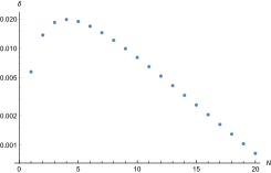
(a) $N_{f}=7$

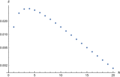
(b) $N_{f}=8$

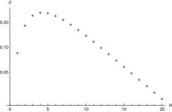
(c) $N_{f}=11$

Figure 3: We show the plot of $\delta$ for $N_{f}=7,8,11$. Note that the vertical axis is log scale.

In (50), we observe that the worldsheet 1-instanton and 2-instanton have no poles in the convergence region $N_{f}>2$ (26). This suggests that there is no “pure” membrane instanton corrections as in the case of 1/2 BPS Wilson loops in ABJM theory HHMO , since there is no need for the membrane instantons to appear to cancel the poles. On the other hand, the worldsheet 3-instanton has a pole at $N_{f}=4$. We conjecture that this pole is canceled by the bound state of order $e^{-2\mu-4\mu/N_{f}}$. It would be interesting to determine the coefficient of this bound state contribution as a function of $N_{f}$.

Also, we observe that the grand canonical VEV (50) has two pieces which scale differently in the large $\mu$ limit: the constant term $-N_{f}/4$ and the remaining part whose leading term gives rise to the perturbative part (43). One can translate this decomposition into the canonical picture

$$W_{\vbox{\offinterlineskip\kern 1.0pt\hbox{\kern 1.0pt\vbox{\hbox{\noindent\vbox{\hbox{\vbox to0.0pt{\hrule height=0.4pt,width=3.90555pt\vss}}\hbox{\vbox{\hbox to0.0pt{\vrule width=0.4pt,height=3.90555pt\hss}}\kern 3.90555pt\vbox{\hbox to0.0pt{\vrule width=0.4pt,height=3.90555pt\hss}}}\hbox{\vbox{\hbox{\vbox to0.0pt{\hrule height=0.4pt,width=4.30554pt\vss}}}\kern-0.4pt}}}\hbox{} }\kern 1.0pt\kern 0.4pt}\kern 1.0pt\kern 0.4pt}}(N,N_{f})=-\frac{N_{f}}{4}Z(N,N_{f})+\widetilde{W}_{\vbox{\offinterlineskip\kern 1.0pt\hbox{\kern 1.0pt\vbox{\hbox{\noindent\vbox{\hbox{\vbox to0.0pt{\hrule height=0.4pt,width=3.90555pt\vss}}\hbox{\vbox{\hbox to0.0pt{\vrule width=0.4pt,height=3.90555pt\hss}}\kern 3.90555pt\vbox{\hbox to0.0pt{\vrule width=0.4pt,height=3.90555pt\hss}}}\hbox{\vbox{\hbox{\vbox to0.0pt{\hrule height=0.4pt,width=4.30554pt\vss}}}\kern-0.4pt}}}\hbox{} }\kern 1.0pt\kern 0.4pt}\kern 1.0pt\kern 0.4pt}}(N,N_{f}),$$ (52)

where the second term behaves in the large $N$ limit as

$$\frac{\widetilde{W}_{\vbox{\offinterlineskip\kern 1.0pt\hbox{\kern 1.0pt\vbox{\hbox{\noindent\vbox{\hbox{\vbox to0.0pt{\hrule height=0.4pt,width=3.90555pt\vss}}\hbox{\vbox{\hbox to0.0pt{\vrule width=0.4pt,height=3.90555pt\hss}}\kern 3.90555pt\vbox{\hbox to0.0pt{\vrule width=0.4pt,height=3.90555pt\hss}}}\hbox{\vbox{\hbox{\vbox to0.0pt{\hrule height=0.4pt,width=4.30554pt\vss}}}\kern-0.4pt}}}\hbox{} }\kern 1.0pt\kern 0.4pt}\kern 1.0pt\kern 0.4pt}}(N,N_{f})}{Z(N,N_{f})}\approx c_{1}(N_{f})e^{\frac{2\mu_{*}}{N_{f}}}.$$ (53)

In section 7, we will show that this decomposition (52) is consistent with the genus-zero result in Grassi:2014vwa .

4.2 Winding number $m=2,3$

Next we consider the worldsheet instanton corrections to the winding Wilson loops $\widehat{W}_{m}(\mu,N_{f})$ for winding numbers $m=2,3$.

Winding number $\boldsymbol{m=2}$

For $m=2$ we find

$$\begin{aligned} \widehat{W}_{2}(\mu,N_{f})=&\frac{2e^{\frac{4\mu}{N_{f}}}}{N_{f}\sin\frac{2\pi}{N_{f}}}\Biggl{[}\frac{1}{4\sin\frac{4\pi}{N_{f}}}+\frac{\cos\frac{2\pi}{N_{f}}(4\mu+N_{f})}{4\pi}e^{-\frac{4\mu}{N_{f}}}\\ &+\Biggl{(}\frac{\sin\frac{4\pi}{N_{f}}(4\mu+N_{f})^{2}}{8\pi^{2}}-\frac{3\cos\frac{4\pi}{N_{f}}(8\mu+N_{f})}{8\pi}+\frac{\cos\frac{2\pi}{N_{f}}\cos\frac{4\pi}{N_{f}}}{\sin\frac{2\pi}{N_{f}}}\Biggr{)}e^{-\frac{8\mu}{N_{f}}}+\mathcal{O}(e^{-\frac{12\mu}{N_{f}}})\Biggl{]}\\ &-C\mu^{2}+B-\frac{8\mu}{\pi N_{f}\sin\frac{2\pi}{N_{f}}}e^{-\frac{4\mu}{N_{f}}}+\mathcal{O}(e^{-\frac{8\mu}{N_{f}}}).\end{aligned}$$ (54)

We observe that the last line of (54) is related to the derivative of the modified grand potential

$$-\partial_{\mu}J(\mu,N_{f})+2B,$$ (55)

where $B$ is the coefficient in the perturbative part (13). As in the case of fundamental representation in the previous subsection, $\widehat{W}_{2}(\mu,N_{f})$ consists of two parts with different scaling behavior in the large $\mu$ limit, which implies that the Wilson loop VEV $W_{2}(N,N_{f})$ in the canonical picture can be decomposed as

$$W_{2}(N,N_{f})=(-N+2B)Z(N,N_{f})+\widetilde{W}_{2}(N,N_{f}),$$ (56)

where the second term in (56) behaves in the large $N$ limit as

$$\frac{\widetilde{W}_{2}(N,N_{f})}{Z(N,N_{f})}\approx c_{2}(N_{f})e^{\frac{4\mu_{*}}{N_{f}}}.$$ (57)

Winding number $\boldsymbol{m=3}$

For $m=3$ we find

$$\begin{aligned} \widehat{W}_{3}(\mu,N_{f})=&\frac{\sin^{2}\frac{\pi}{N_{f}}}{\sin\frac{2\pi}{N_{f}}\sin\frac{4\pi}{N_{f}}}e^{\frac{6\mu}{N_{f}}}\Biggl{[}\frac{1}{4\sin\frac{6\pi}{N_{f}}}-\frac{\sin\frac{3\pi}{N_{f}}}{\sin\frac{\pi}{N_{f}}}\frac{(4\mu+N_{f})}{4\pi}e^{-\frac{4\mu}{N_{f}}}\\ &+\Biggl{(}\frac{\sin\frac{6\pi}{N_{f}}(4\mu+N_{f})^{2}}{8\pi^{2}}-\frac{3\cos\frac{2\pi}{N_{f}}\sin^{2}\frac{3\pi}{N_{f}}}{\sin^{2}\frac{\pi}{N_{f}}}\frac{(8\mu+N_{f})}{8\pi}\\ &+\frac{\sin\frac{3\pi}{N_{f}}\cos\frac{2\pi}{N_{f}}}{\sin\frac{\pi}{N_{f}}\sin\frac{2\pi}{N_{f}}}\Bigl{(}\cos\frac{4\pi}{N_{f}}-\cos\frac{2\pi}{N_{f}}-1\Bigr{)}\Biggr{)}e^{-\frac{8\mu}{N_{f}}}+\mathcal{O}(e^{-\frac{12\mu}{N_{f}}})\Biggr{]}\\ &-\frac{N_{f}}{4}+3e^{\frac{2\mu}{N_{f}}}\Biggl{[}\frac{1}{4\sin\frac{2\pi}{N_{f}}}+\frac{4\mu+N_{f}}{4\pi}e^{-\frac{4\mu}{N_{f}}}+\mathcal{O}(e^{-\frac{8\mu}{N_{f}}})\Biggr{]}.\end{aligned}$$ (58)

In this case, we observe that $\widehat{W}_{3}(\mu,N_{f})$ consists of three parts with different scalings in the large $\mu$ limit. Noticing that the last term of (58) is proportional to $\widetilde{W}_{\vbox{\offinterlineskip\kern 1.0pt\hbox{\kern 1.0pt\vbox{\hbox{\noindent\vbox{\hbox{\vbox to0.0pt{\hrule height=0.4pt,width=3.90555pt\vss}}\hbox{\vbox{\hbox to0.0pt{\vrule width=0.4pt,height=3.90555pt\hss}}\kern 3.90555pt\vbox{\hbox to0.0pt{\vrule width=0.4pt,height=3.90555pt\hss}}}\hbox{\vbox{\hbox{\vbox to0.0pt{\hrule height=0.4pt,width=4.30554pt\vss}}}\kern-0.4pt}}}\hbox{} }\kern 1.0pt\kern 0.4pt}\kern 1.0pt\kern 0.4pt}}$ in (50), we conjecture that the canonical VEV $W_{3}(N,N_{f})$ for winding number $m=3$ is decomposed as

$$\begin{aligned} W_{3}(N,N_{f})=-\frac{N_{f}}{4}Z(N,N_{f})+3\widetilde{W}_{\vbox{\offinterlineskip\kern 1.0pt\hbox{\kern 1.0pt\vbox{\hbox{\noindent\vbox{\hbox{\vbox to0.0pt{\hrule height=0.4pt,width=3.90555pt\vss}}\hbox{\vbox{\hbox to0.0pt{\vrule width=0.4pt,height=3.90555pt\hss}}\kern 3.90555pt\vbox{\hbox to0.0pt{\vrule width=0.4pt,height=3.90555pt\hss}}}\hbox{\vbox{\hbox{\vbox to0.0pt{\hrule height=0.4pt,width=4.30554pt\vss}}}\kern-0.4pt}}}\hbox{} }\kern 1.0pt\kern 0.4pt}\kern 1.0pt\kern 0.4pt}}(N,N_{f})+\widetilde{W}_{3}(N,N_{f}),\end{aligned}$$ (59)

where the last term scales as

$$\frac{\widetilde{W}_{3}(N,N_{f})}{Z(N,N_{f})}\approx c_{3}(N_{f})e^{\frac{6\mu_{*}}{N_{f}}}.$$ (60)

We have confirmed our result of instanton corrections (54) and (58) for $m=2,3$ by performing a similar test as in Fig. 3. We have checked a correct exponential decay of the quantity $\delta$ for various $N_{f}$’s in the convergence region (26).

5 WKB expansion

In this section, we will consider the WKB expansion (small $\hbar$ expansion) of spectral trace $\operatorname{Tr}(\rho^{s}e^{x})$ and try to reproduce the perturbative part of fundamental representation. Our starting point is the Mellin-Barnes representation of the grand canonical VEV Hatsuda:2015oaa ; Marino:2016new

$$\widehat{W}_{\vbox{\offinterlineskip\kern 1.0pt\hbox{\kern 1.0pt\vbox{\hbox{\noindent\vbox{\hbox{\vbox to0.0pt{\hrule height=0.4pt,width=3.90555pt\vss}}\hbox{\vbox{\hbox to0.0pt{\vrule width=0.4pt,height=3.90555pt\hss}}\kern 3.90555pt\vbox{\hbox to0.0pt{\vrule width=0.4pt,height=3.90555pt\hss}}}\hbox{\vbox{\hbox{\vbox to0.0pt{\hrule height=0.4pt,width=4.30554pt\vss}}}\kern-0.4pt}}}\hbox{} }\kern 1.0pt\kern 0.4pt}\kern 1.0pt\kern 0.4pt}}(\mu,N_{f})=\int_{c-{\rm i}\infty}^{c+{\rm i}\infty}\frac{ds}{2\pi{\rm i}}\frac{\pi}{\sin\pi s}\operatorname{Tr}(\rho^{s}e^{x})e^{s\mu},$$ (61)

where $c$ is a positive constant in the region $2/N_{f}<c<1$. By picking up the poles at $s=\ell\in\mathbb{N}$ we recover the small $\kappa$ expansion (30). On the other hand, closing the contour in the direction $\text{Re}(s)<c$ we can find the large $\mu$ expansion of $\widehat{W}_{\vbox{\offinterlineskip\kern 1.0pt\hbox{\kern 1.0pt\vbox{\hbox{\noindent\vbox{\hbox{\vbox to0.0pt{\hrule height=0.4pt,width=3.90555pt\vss}}\hbox{\vbox{\hbox to0.0pt{\vrule width=0.4pt,height=3.90555pt\hss}}\kern 3.90555pt\vbox{\hbox to0.0pt{\vrule width=0.4pt,height=3.90555pt\hss}}}\hbox{\vbox{\hbox{\vbox to0.0pt{\hrule height=0.4pt,width=4.30554pt\vss}}}\kern-0.4pt}}}\hbox{} }\kern 1.0pt\kern 0.4pt}\kern 1.0pt\kern 0.4pt}}(\mu,N_{f})$.

In the quantum mechanical description of density matrix (6), the Planck constant is fixed to $\hbar=2\pi$ (7). However, one can formally introduce the parameter $\hbar$ in the canonical commutation relation $[\widehat{x},\widehat{p}]={\rm i}\hbar$ and perform the WKB expansion of the spectral trace $\operatorname{Tr}(\rho^{s}e^{x})$. Finally we set $\hbar=2\pi$ at the end of computation. This procedure was successfully applied to several examples Assel:2015hsa ; Okuyama:2015auc .

At the zero-th order of WKB expansion, the spectral trace is given by the classical phase space integral

$$Z_{0}(s)=\int\frac{dxdp}{2\pi\hbar}\left[\frac{1}{2\cosh\frac{p}{2}}\frac{1}{(2\cosh\frac{x}{2})^{N_{f}}}\right]^{s}e^{x}=\frac{\Gamma\big{(}\frac{s}{2}\big{)}^{2}\Gamma\Big{(}\frac{N_{f}s}{2}+1\Big{)}\Gamma\Big{(}\frac{N_{f}s}{2}-1\Big{)}}{2\pi\hbar\Gamma(s)\Gamma(N_{f}s)},$$ (62)

and the higher order corrections can be systematically computed by using the Wigner transformation of operator $\hat{\rho}^{s}e^{\widehat{x}}$ Hatsuda:2015lpa ; Okuyama:2015auc ; Okuyama:2016xke ; Okuyama:2016deu . In this way, we find the WKB expansion of spectral trace as

$$\begin{aligned} \operatorname{Tr}(\rho^{s}x^{x})=Z_{0}(s)D(s),\end{aligned}$$ (63)

where $D(s)$ is a formal power series in $\hbar$

$$D(s)=1+\sum_{n=1}^{\infty}\hbar^{2n}D_{n}(s).$$ (64)

We find that the $n^{\text{th}}$ order term $D_{n}(s)$ has the following structure:

$$D_{n}(s)=\frac{(s-1)p_{n}(s)}{\prod_{j=1}^{n}(N_{f}s+2j-1)},$$ (65)

where $p_{n}(s)$ is a $(3n-1)^{\text{th}}$ order polynomial of $s$. The first three terms are given by

$$\begin{aligned} p_{1}(s)&=c_{1}(N_{f}^{2}s^{2}-4N_{f}s-8),\\ p_{2}(s)&=c_{2}\Biggl{[}N_{f}^{4}s^{5}+\frac{1}{7}N_{f}^{3}(3N_{f}-32)s^{4}+\frac{8}{7}N_{f}^{2}\left(N_{f}^{2}-2N_{f}-18\right)s^{3}\\ &\quad-\frac{16}{7}N_{f}\left(4N_{f}^{2}+5N_{f}-24\right)s^{2}-\frac{128}{7}\left(3N_{f}^{2}-N_{f}-9\right)s+\frac{384}{7}\Biggr{]},\\ p_{3}(s)&=c_{3}\Biggl{[}N_{f}^{6}s^{8}+\frac{4}{31}N_{f}^{5}(16N_{f}-15)s^{7}+\frac{1}{31}N_{f}^{4}\left(129N_{f}^{2}-176N_{f}-1544\right)s^{6}\\ &\qquad+\frac{4}{31}N_{f}^{3}\left(18N_{f}^{3}-129N_{f}^{2}-944N_{f}+288\right)s^{5}\\ &\qquad+\frac{8}{31}N_{f}^{2}\left(16N_{f}^{4}-44N_{f}^{3}-1275N_{f}^{2}-80N_{f}+2640\right)s^{4}\\ &\qquad+\frac{64}{31}N_{f}\left(2N_{f}^{5}-24N_{f}^{4}-103N_{f}^{3}-53N_{f}^{2}+540N_{f}-72\right)s^{3}\\ &\qquad-\frac{128}{31}\left(12N_{f}^{5}+120N_{f}^{4}-32N_{f}^{3}-955N_{f}^{2}+48N_{f}+1080\right)s^{2}\\ &\qquad-\frac{1024}{31}\left(15N_{f}^{4}-120N_{f}^{2}+N_{f}+180\right)s-\frac{30720}{31}\Biggr{]}.\end{aligned}$$ (66)

The coefficient $c_{n}$ of the highest order term $N_{f}^{2n}s^{3n-1}$ in $p_{n}(s)$ (66) is found to be

$$c_{n}=\frac{B_{2n}(1/2)}{2^{4n}(2n)!},$$ (67)

where $B_{2n}(1/2)$ denotes the Bernoulli polynomial $B_{2n}(z)$ evaluated at $z=1/2$. We have computed $D_{n}(s)$ up to $n_{\text{max}}=10$.

As mentioned above, the large $\mu$ expansion of grand canonical VEV can be found by closing the contour of (61) in the direction $\text{Re(s)}<c$. The perturbative part comes from the pole at $s=2/N_{f}$ of $Z_{0}(s)$ in (62)

$$\text{Res}_{s=\frac{2}{N_{f}}}\left[\frac{\pi}{\sin\pi s}Z_{0}(s)D(s)e^{s\mu}\right]=\frac{1}{N_{f}\hbar\sin\frac{2\pi}{N_{f}}}\frac{\Gamma\bigl{(}\frac{1}{N_{f}}\bigr{)}^{2}}{\Gamma\bigl{(}\frac{2}{N_{f}}\bigr{)}}D\Bigl{(}\frac{2}{N_{f}}\Bigr{)}e^{\frac{2\mu}{N_{f}}}.$$ (68)

In order to reproduce the coefficient $c_{1}(N_{f})$ of the perturbative part of fundamental representation in (48), we need to show that

$$D\Bigl{(}\frac{2}{N_{f}}\Bigr{)}=\frac{\pi N_{f}\Gamma\bigl{(}\frac{2}{N_{f}}\bigr{)}}{2\Gamma\bigl{(}\frac{1}{N_{f}}\bigr{)}^{2}}.$$ (69)

Although we do not have an analytic proof of this relation, we can check this numerically by using the Padé approximation

$$D(s)\approx 1+\sum_{n=1}^{n_{\text{max}}}\hbar^{2n}D_{n}(s)\approx\frac{1+a_{1}\hbar^{2}+\cdots+a_{n_{\text{max}/2}}\hbar^{n_{\text{max}}}}{1+b_{1}\hbar^{2}+\cdots+b_{n_{\text{max}/2}}\hbar^{n_{\text{max}}}},$$ (70)

and set $\hbar=2\pi$ at the end. As we can see from Fig. 4(a), the Padé approximation exhibits a nice agreement with the expected behavior in (69).

One can also repeat the same analysis for the constant part $-N_{f}/4$ in (50), which comes from the pole at $s=0$ in (61)

$$\text{Res}_{s=0}\left[\frac{\pi}{\sin\pi s}Z_{0}(s)D(s)e^{s\mu}\right]=-\frac{2D(0)}{\pi\hbar}(2\mu+N_{f})-\frac{4D^{\prime}(0)}{\pi\hbar}.$$ (71)

From the first few terms of the expansion of $D(0)$, one can easily guess the closed form of $D(0)$

$$D(0)=1-\frac{\hbar^{2}}{48}-\frac{\hbar^{4}}{11520}-\frac{\hbar^{6}}{1935360}+\cdots=\frac{\hbar}{4}\cot\frac{\hbar}{4}.$$ (72)

After setting $\hbar=2\pi$, we find $D(0)=0$ as expected. In order to reproduce the constant $-N_{f}/4$, we need

$$D^{\prime}(0)=\frac{\pi^{2}N_{f}}{8}.$$ (73)

Again, we can check this relation numerically using the Padé approximation for $D^{\prime}(0)$. We find a nice agreement with the right hand side of (73) (see Fig. 4(b)).

We expect that the worldsheet $\ell$-instanton comes from the pole at $s=(2-4\ell)/N_{f}$. In principle, we can find the instanton coefficients from the WKB analysis. However, it is difficult in practice since both the classical part $Z_{0}(s)$ and the quantum corrections $D(s)$ should have poles at $s=(2-4\ell)/N_{f}$ in order to reproduce the Fermi gas result (50). This is different from the situation for the perturbative part and the constant term considered above, where the poles only come from the classical part. By the same reason, it is difficult to study the winding Wilson loop $\widehat{W}_{m}(\mu,N_{f})$ with $m\geq 2$ from the WKB analysis.

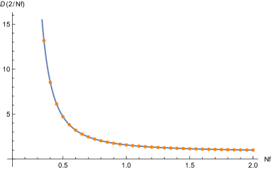
(a) plot of $D(2/N_{f})$

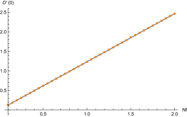
(b) plot of $D^{\prime}(0)$

Figure 4: We show the plot of 4(a) $D(2/N_{f})$ and 4(b) $D^{\prime}(0)$, against $N_{f}$. The dots are the numerical values obtained from the Padé approximation, while the solid curves represent the exact functions in (69) and (73) for 4(a) and 4(b), respectively.

6 Planar solution of $N_{f}$ matrix model

In this section, we will summarize the planar solution of the $N_{f}$ matrix model. This section is mostly a review of the result in Grassi:2014vwa , but we find that the the planar resolvent in Grassi:2014vwa can be vastly simplified. Using this simplified expression of resolvent, we will directly show that the resolvent satisfies the planar loop equation without referring to the relation to the $O(n)$ matrix model EK1 ; EK2 ; Suyama:2012uu .

Let us consider the planar resolvent of $N_{f}$ matrix model in the ’t Hooft limit (1)

$$\omega(z)=\frac{1}{Z(N,N_{f})}\Biggl{\langle}\frac{1}{N_{f}}\sum_{i=1}^{N}\frac{z+e^{x_{i}}}{z-e^{x_{i}}}\Biggr{\rangle},$$ (74)

where we have normalized the VEV (25) by the partition function. In the ’t Hooft limit (1), the eigenvalue distribution becomes continuous. Since the integrand of the $N_{f}$ matrix model (3) is an even function of $x_{i}$, the eigenvalues are distributed symmetrically around the origin $x_{i}\in[-T,T]$. Noticing that the variable $z$ in (74) is related to the eigenvalue $x$ by $z=e^{x}$, $\omega(z)$ is expected to have a cut along $z\in[a,b]$ with $a=e^{-T},b=e^{T}$.

The resolvent $\omega(z)$ should satisfy several conditions. First of all, $\omega(z)$ should satisfy the loop equation which comes from the saddle point equation of matrix integral (3)

$$\omega(z+{\rm i}0)+\omega(z-{\rm i}0)-2\omega(-z)=V^{\prime}(z)$$ (75)

along the cut $z\in[a,b]$. Here $V^{\prime}(z)$ is given by

$$V^{\prime}(z)=\frac{z-1}{z+1}.$$ (76)

Also, from the definition (74) and the symmetry of the eigenvalue distribution we find

$$\omega(0) =-\lambda,$$ (77)

$$\omega(z^{-1}) =-\omega(z).$$ (78)

Mapping to the torus $\mathbb{C}/(\mathbb{Z}+\tau\mathbb{Z})$

To find the resolvent, it is convenient to map $z$ to the variable $u$ by a Jacobi elliptic function

$$z=a\,\text{sn}(u,k),$$ (79)

where the elliptic modulus $k$ is given by

$$k=\frac{a}{b}=a^{2}.$$ (80)

In what follows we will suppress the dependence of $k$. We also need the derivative of $z$

$$\partial_{u}z=a\,\text{cn}(u)\text{dn}(u)=a\sqrt{(1-a^{2}z^{2})(1-a^{-2}z^{2})}.$$ (81)

Furthermore, the variable $u$ is related to the flat coordinate $v$ on the torus $\mathbb{C}/(\mathbb{Z}+\tau\mathbb{Z})$ by

$$v=\frac{u}{2K},$$ (82)

where $K=K(k^{2})$ is the elliptic integral of the first kind and the complex structure of the torus is given by

$$\tau=\frac{{\rm i}K^{\prime}}{K}.$$ (83)

Then the coordinate $z$ and the end-point of the cut $a$ is written in terms of the Jacobi theta functions

$$\begin{aligned} z&=\frac{\vartheta_{1}(v,\tau)}{\vartheta_{4}(v,\tau)},\\ a&=\frac{\vartheta_{2}(0,\tau)}{\vartheta_{3}(0,\tau)}.\end{aligned}$$ (84)

We will use the variables $z,u$ and $v$ interchangeably. One can show that $z(v)$ satisfies

$$\begin{aligned} &z(-v)=-z(v),\\ &z(v+1)=-z(v),\\ &z(v+\tau)=z(v),\\ &z\Big{(}v+\frac{\tau}{2}\Big{)}=\frac{1}{z(v)},\\ &z\Big{(}v+\frac{1}{2}\Big{)}=a\sqrt{\frac{1-a^{-2}z(v)^{2}}{1-a^{2}z(v)^{2}}}=\frac{\vartheta_{2}(v,\tau)}{\vartheta_{3}(v,\tau)},\end{aligned}$$ (85)

and the various points on the $z$-plane are mapped to the points on the $v$-plane as

$z$	0	$\infty$	$a$	$a^{-1}$	$\pm 1$	$\pm{\rm i}$
$v$	0	$\frac{\tau}{2}$	$\frac{1}{2}$	$\frac{1}{2}+\frac{\tau}{2}$	$\pm\frac{1}{2}+\frac{\tau}{4}$	$\pm\frac{\tau}{4}$

Conditions obeyed by the resolvent $\boldsymbol{\omega(v)}$

Here we will write down the conditions for the resolvent $\omega(v)$ in terms of the variable $v$. The loop equation becomes

$$\omega\Bigl{(}\frac{1}{2}+v\Bigr{)}+\omega\Bigl{(}\frac{1}{2}-v\Bigr{)}-2\omega\Bigl{(}-\frac{1}{2}-v\Bigr{)}=V^{\prime}\Bigl{(}\frac{1}{2}+v\Bigr{)},\quad\text{for}~{}v\in[0,\frac{\tau}{2}].$$ (86)

We also require that there are no cuts along $z\in[-b,-a]$ and $z\in[-\infty,-b]\cup[b,\infty]$. In terms of the variable $v$ these conditions become

$$\begin{aligned} \omega\Bigl{(}-\frac{1}{2}+v\Bigr{)}&=\omega\Bigl{(}-\frac{1}{2}-v\Bigr{)},\quad\text{for}~{}v\in[0,\frac{\tau}{2}],\\ \omega\Bigl{(}\frac{\tau}{2}+v\Bigr{)}&=\omega\Bigl{(}-\frac{\tau}{2}+v\Bigr{)},\quad\text{for}~{}v\in[-\frac{1}{2},\frac{1}{2}].\end{aligned}$$ (87)

Using the above conditions, $\omega(v)$ can be extended to a function on the torus obeying the following functional relations

$$\omega(v+1)+\omega(v-1)-2\omega(v)=V^{\prime}(v+1),$$ (88)

$$\omega\Bigl{(}-\frac{1}{2}+v\Bigr{)}=\omega\Bigl{(}-\frac{1}{2}-v\Bigr{)},$$ (89)

$$\omega(v+\tau)=\omega(v).$$ (90)

6.1 Planar resolvent

The resolvent $\omega(v)$ was obtained in Grassi:2014vwa by taking a limit of the solution of $O(n)$ matrix model EK1 ; EK2 ; Suyama:2012uu . After massaging the expression in Grassi:2014vwa , we find a very simple formula for the resolvent

$$\omega(z)=\frac{\widetilde{A}(z)^{2}}{2\pi^{2}}\frac{z^{2}+1}{z^{2}-1}-\frac{1}{4}\frac{z+1}{z-1}+\widehat{\lambda}\,\frac{z^{2}-1}{z^{2}+1}.$$ (91)

The function $\widetilde{A}(z)$ in (91) is given by

$$\widetilde{A}(z)=\frac{\pi}{2}+A(u)-K^{\prime}\frac{\partial_{u}z}{z(1+z^{2})},$$ (92)

where $K^{\prime}=K(1-k^{2})$ and $A(u)$ denotes the function introduced in Grassi:2014vwa

$$A(u)=\frac{\pi u}{2K}+K^{\prime}Z(u)+K^{\prime}\partial_{u}\log z,$$ (93)

with $Z(u)$ being the Jacobi zeta function

$$Z(u)=\partial_{u}\log\vartheta_{4}\Bigl{(}\frac{u}{2K},\tau\Bigr{)}.$$ (94)

In terms of the variable $v$, we find that $\widetilde{A}(v)$ in (91) is written as

$$\begin{aligned} \widetilde{A}(v)&=\frac{\pi}{2}+\pi v-\frac{{\rm i}\tau}{2}\partial_{v}\log\vartheta_{4}(v,\tau)-\frac{{\rm i}\tau}{4}\partial_{v}\log(1+z^{2})\\ &=\frac{\pi}{2}+\pi v-\frac{{\rm i}\tau}{4}\partial_{v}\log\Bigl{[}\vartheta_{1}(v,\tau)^{2}+\vartheta_{4}(v,\tau)^{2}\Bigr{]}.\end{aligned}$$ (95)

One can remove the linear term of $v$ by performing the modular S-transformation

$$\widetilde{A}(z)=-\frac{{\rm i}}{4}\partial_{v^{\prime}}\log\Biggl{[}\vartheta_{3}\Bigl{(}v^{\prime}+\frac{\tau^{\prime}}{2},\tau^{\prime}\Bigr{)}^{2}+\vartheta_{4}\Bigl{(}v^{\prime}+\frac{\tau^{\prime}}{2},\tau^{\prime}\Bigr{)}^{2}\Biggr{]}$$ (96)

with

$$v^{\prime}=\frac{v}{\tau},\quad\tau^{\prime}=-\frac{1}{\tau}.$$ (97)

As discussed in Borot:2009ia , we could use the S-dual variables $(v^{\prime},\tau^{\prime})$ from the beginning. However, we will not do so and we will continue to use the original variables $(v,\tau)$.

In the following, we will show that $\omega(z)$ in (91) indeed satisfies the necessary functional relations.

Symmetries of $\boldsymbol{\omega(v)}$

First, let us consider the relation (78). In terms of $v$, (78) is written as

$$\omega\Bigl{(}v+\frac{\tau}{2}\Bigr{)}=-\omega(v).$$ (98)

This is satisfied since $z(v+\tau/2)=1/z(v)$ and

$$\widetilde{A}\Bigl{(}v+\frac{\tau}{2}\Bigr{)}=\widetilde{A}(v),$$ (99)

which follows from the identity of Jacobi theta functions

$$\vartheta_{4}\Bigl{(}v+\frac{\tau}{2},\tau\Bigr{)}={\rm i}e^{-\pi{\rm i}(v+\frac{\tau}{4})}\vartheta_{1}(v,\tau),\quad\vartheta_{1}\Bigl{(}v+\frac{\tau}{2},\tau\Bigr{)}={\rm i}e^{-\pi{\rm i}(v+\frac{\tau}{4})}\vartheta_{4}(v,\tau).$$ (100)

Then, the $\tau/2$-shift relation (98) implies that $\omega(v)$ is periodic (90) with period $\tau$. One can also show the relation (89) by using

$$\begin{aligned} \widetilde{A}\Bigl{(}-\frac{1}{2}+v\Bigr{)}&=-\widetilde{A}\Bigl{(}-\frac{1}{2}-v\Bigr{)},\\ z\Bigl{(}-\frac{1}{2}+v\Bigr{)}&=z\Bigl{(}-\frac{1}{2}-v\Bigr{)}.\end{aligned}$$ (101)

Next let us consider the normalization condition (77). So far $\widehat{\lambda}$ in (91) is just a formal parameter in the ansatz of solution. The relation between $\widehat{\lambda}$ and the ’t Hooft coupling $\lambda$ is fixed by the condition (77). Using $\widetilde{A}(0)=\pi/2$, we find

$$\widehat{\lambda}=\lambda+\frac{1}{8}.$$ (102)

This shift by $1/8$ is consistent with the Fermi gas result (13)

$$N-B=N_{f}\left(\lambda+\frac{1}{8}\right)-\frac{1}{2N_{f}},$$ (103)

at the leading order in the ’t Hooft limit.

Absence of poles at $\boldsymbol{z=\pm 1}$

We also want to show that the resolvent is regular at $z=\pm 1$. This requires

$$\widetilde{A}\Bigl{(}\frac{1}{2}+\frac{\tau}{4}\Bigr{)}=\pi,\qquad\widetilde{A}\Bigl{(}-\frac{1}{2}+\frac{\tau}{4}\Bigr{)}=0.$$ (104)

One can show that (104) is satisfied by using

$$\begin{aligned} \partial_{v}z\big{|}_{z=\pm 1}&=2{\rm i}(a^{2}-1)K,\\ \partial_{v}\log\vartheta_{4}\Bigl{(}\pm\frac{1}{2}+\frac{\tau}{4}\Bigr{)}&=-\frac{{\rm i}\pi}{2}\pm{\rm i}(1-a^{2})K.\end{aligned}$$ (105)

The second equality in (105) is a consequence of the formula in the Appendix A of Grassi:2014vwa .

Absence of poles at $\boldsymbol{z=\pm{\rm i}}$

The regularity of resolvent at $z=\pm{\rm i}$ determines $\widehat{\lambda}$ as a function of $a$. One can show that $A(u)$ in (92) is regular at $z=\pm{\rm i}$, and hence near $z=\pm{\rm i}$ the resolvent behaves as

$$\lim_{z\to\pm{\rm i}}\omega(z)=\frac{1}{2\pi^{2}}\left(\frac{K^{\prime}\partial_{u}z}{z(z^{2}+1)}\right)^{2}\frac{z^{2}+1}{z^{2}-1}+\widehat{\lambda}\frac{z^{2}-1}{z^{2}+1}+(\text{regular}).$$ (106)

From this behavior, the condition for the absence of pole at $z=\pm{\rm i}$ is found to be

$$\widehat{\lambda}=\frac{t^{2}}{8\pi^{2}},$$ (107)

where $t$ is given by

$$t=K^{\prime}\partial_{u}z\Big{|}_{z=\pm{\rm i}}.$$ (108)

Using (81) we find that $t$ is written as

$$t=(1+a^{2})K^{\prime}.$$ (109)

This reproduces the result in Grassi:2014vwa .

Loop equation

Finally, let us show that $\omega(v)$ in (91) satisfies the loop equation (88). In Grassi:2014vwa , this was shown implicitly by taking a limit of the resolvent of $O(n)$ matrix model. Here we will show the loop equation (88) directly.

To do this, it is convenient to introduce the operator $\textbf{T}^{\pm}$ shifting $v$ by $\pm 1$

$$\textbf{T}^{\pm}\,\omega(v)=\omega(v\pm 1).$$ (110)

Then the planar loop equation is written as

$$\textbf{L}\,\omega(v)=V^{\prime}(-z),$$ (111)

where L is given by

$$\textbf{L}=\textbf{T}+\textbf{T}^{-1}-2.$$ (113)

On the right hand side of (111), we have also used $\textbf{T}\cdot z=-z$ and $V^{\prime}(v+1)=V^{\prime}(-z)$.

For a rational function $f(z)$ of $z$, the action of L reads

$$\textbf{L}\,f(z)=2f(-z)-2f(z).$$ (114)

However, we should be careful about $\widetilde{A}(z)$ which transforms inhomogeneously under $\textbf{T}^{\pm}$

$$\textbf{T}^{\pm}\,\widetilde{A}(z)=\widetilde{A}(z)\pm\pi,$$ (115)

due to the linear term $\pi v$ in (95). Then we find

$$\textbf{L}\,\widetilde{A}(z)^{2}=\big{(}\widetilde{A}(z)+\pi\big{)}^{2}+\big{(}\widetilde{A}(z)-\pi\big{)}^{2}-2\widetilde{A}(z)^{2}=2\pi^{2}.$$ (116)

Now we are ready to prove (88). It is natural to decompose $\omega(z)$ in (91) into three parts

$$\omega(z)=\omega_{1}(z)+\omega_{2}(z)+\omega_{3}(z),$$ (117)

where

$$\begin{aligned} \omega_{1}(z)&=\frac{\widetilde{A}(z)^{2}}{2\pi^{2}}\frac{z^{2}+1}{z^{2}-1}=\frac{\widetilde{A}(z)^{2}}{4\pi^{2}}\Bigl{[}V^{\prime}(z)+V^{\prime}(-z)\Bigr{]},\\ \omega_{2}(z)&=-\frac{1}{4}V^{\prime}(-z),\\ \omega_{3}(z)&=\widehat{\lambda}\,\frac{z^{2}-1}{z^{2}+1}.\end{aligned}$$ (118)

One can easily show that the action of L on $\omega_{1,2,3}$ is given by

$$\begin{aligned} \textbf{L}\,\omega_{1}(z)&=\frac{1}{2}\Bigl{[}V^{\prime}(z)+V^{\prime}(-z)\Bigr{]},\\ \textbf{L}\,\omega_{2}(z)&=-\frac{1}{2}\Bigl{[}V^{\prime}(z)-V^{\prime}(-z)\Bigr{]},\\ \textbf{L}\,\omega_{3}(z)&=0.\end{aligned}$$ (119)

where we have used (116) in the first line. Adding these three equations (119), finally we arrive at the desired loop equation (111).

6.2 Planar free energy

In Grassi:2014vwa , the second derivative of the planar free energy is found explicitly as

$$\frac{\partial^{2}F_{0}}{\partial\lambda^{2}}=-\frac{2\pi K}{K^{\prime}}=-\frac{2\pi{\rm i}}{\tau}.$$ (120)

From (107), (109) and (120), we find that the derivative of $\lambda$ and $\frac{\partial F_{0}}{\partial\lambda}$ with respect to $t$ have a simple form

$$\begin{aligned} \frac{\partial\lambda}{\partial t}&=\frac{t}{4\pi^{2}}=\frac{(1+a^{2})K^{\prime}}{4\pi^{2}},\\ \frac{\partial^{2}F_{0}}{\partial t\partial\lambda}&=-\frac{(1+a^{2})K}{2\pi}.\end{aligned}$$ (121)

Note that the role of A-period and B-period is opposite from the standard definition. Using this relation (121), one can find the planar free energy $F_{0}$ as a function of ’t Hooft coupling $\lambda$. In particular, in the small $\lambda$ or large $\lambda$ regime $F_{0}$ can be explicitly found as a power series.

Let us first consider the large $\lambda$ behavior of $F_{0}$. In the large $\lambda$ limit the size of the cut $[-T,T]$ in the original variable $x$ becomes large, which implies $a=e^{-T}\to 0$. More precisely, we find that the large $t$ expansion of $a$ is given by

$$a=2e^{-\frac{t}{2}}\Biggl{[}1+2te^{-t}+2(5t^{2}-3t-1)e^{-2t}+\frac{4t}{3}(49t^{2}-63t-3)e^{-3t}+\mathcal{O}(e^{-4t})\Biggr{]}.$$ (122)

Note that $t$ and the shifted ’t Hooft coupling $\widehat{\lambda}=\lambda+1/8$ are related by (107) and the exponential correction $e^{-t}$ in (122) is identified with the worldsheet instanton factor (21)

$$e^{-t}=e^{-2\pi\sqrt{2\widehat{\lambda}}}.$$ (123)

Then, integrating the relation (121) the planar free energy becomes

$$-F_{0}=\frac{t^{3}}{48\pi^{2}}-a_{0}+\frac{t+1}{4\pi^{2}}e^{-t}+\frac{8t^{2}+14t+7}{32\pi^{2}}e^{-2t}+\frac{18t^{3}+27t^{2}+21t+7}{27\pi^{2}}e^{-3t}+\mathcal{O}(e^{-4t}),$$ (124)

where $a_{0}$ is a constant coming from the constant term $A$ in the perturbative part (12) of grand potential HO

$$a_{0}=\lim_{N_{f}\to\infty}\frac{A}{N_{f}^{2}}=-\frac{\zeta(3)}{8\pi^{2}}+\frac{1}{8}\log 2.$$ (125)

On the other hand, in the small $\lambda$ limit the size of cut $[-T,T]$ in the $x$-variable becomes small, which implies $a\to 1$. From (107) and (109), we find that the small $\lambda$ expansion of $\log a$ is given by

$$\log a=-4\sqrt{\lambda}\left(1-\frac{\lambda}{6}+\frac{43\lambda^{2}}{40}-\frac{621\lambda^{3}}{112}+\frac{35027\lambda^{4}}{1152}+\mathcal{O}(\lambda^{5})\right),$$ (126)

and the free energy becomes

$$-F_{0}=-\frac{\lambda^{2}}{2}\log\lambda+\frac{3\lambda^{2}}{4}+\frac{\lambda^{3}}{2}-\frac{19\lambda^{4}}{24}+\frac{9\lambda^{5}}{4}-\frac{991\lambda^{6}}{120}+\mathcal{O}(\lambda^{7}).$$ (127)

7 ’t Hooft limit of Wilson loops

In this section, we consider the ’t Hooft expansion of normalized Wilson loop VEV

$$\frac{W_{m}(N,N_{f})}{Z(N,N_{f})}=\sum_{g=0}^{\infty}N_{f}^{1-2g}W_{m}^{(g)}.$$ (128)

Note that our normalization of VEV is different from Grassi:2014vwa (see footnote 2 for our definition). As we will see below, we find a perfect agreement between the matrix model result and the Fermi gas result for the genus-zero part $W_{m}^{(g=0)}$ of Wilson loop in (128).

7.1 Results of matrix model

We can read off the genus-zero VEV of Wilson loops from the small $z$ expansion of the resolvent (91)

$$\omega(z)=-\lambda-2\sum_{m=1}^{\infty}W_{m}^{(g=0)}z^{m}.$$ (130)

To write down the small $z$ expansion of $\omega(z)$ in (91), let us first consider the small $u$ expansion of $\widetilde{A}(z)$ in (92)

$$\widetilde{A}(z)=\frac{\pi}{2}+Iu+t\Bigl{[}-\frac{2}{3}a^{2}\left(a^{2}+1\right)u^{3}+\frac{2}{15}a^{2}\left(a^{2}+1\right)\left(a^{4}+6a^{2}+1\right)u^{5}+\mathcal{O}(u^{7})\Bigr{]},$$ (131)

where $t$ is defined in (109) and the factor $I$ is given by

$$I=\frac{\pi}{2K}+t\left(1-\frac{E}{(1+a^{2})K}\right).$$ (132)

Here $E=E(k^{2})$ denotes the elliptic integral of the second kind. By inverting the relation $z=a\,\text{sn}(u)$ in (79), we can write down the small $z$ expansion of $u$

$$u=\frac{z}{a}+\frac{\left(a^{4}+1\right)z^{3}}{6a^{3}}+\frac{\left(3a^{8}+2a^{4}+3\right)z^{5}}{40a^{5}}+\mathcal{O}(z^{7}).$$ (133)

Combining (131) and (133), we find that $\widetilde{A}(z)$ is expanded as

$$\begin{aligned} \widetilde{A}(z)&=\frac{\pi}{2}+\frac{I}{a}z+\Biggl{[}\frac{\left(a^{4}+1\right)I}{6a^{3}}-\frac{2\left(a^{2}+1\right)t}{3a}\Biggr{]}z^{3}\\ &+\Biggl{[}\frac{\left(3a^{8}+2a^{4}+3\right)I}{40a^{5}}-\frac{\left(a^{2}+1\right)\left(a^{4}-4a^{2}+1\right)t}{5a^{3}}\Biggr{]}z^{5}+\mathcal{O}(z^{7}).\end{aligned}$$ (134)

We notice that the coefficients in this expansion (134) are some linear combinations of $I$ and $t$. Plugging this expansion (134) into (91) and read off the coefficient of $z^{m}$ in (130), we can find the planar VEV of winding Wilson loops $W_{m}^{(g=0)}$ up to arbitrary winding number $m$, in principle. For instance, the planar VEV of Wilson loop in the fundamental representation is given by

$$W_{\vbox{\offinterlineskip\kern 1.0pt\hbox{\kern 1.0pt\vbox{\hbox{\noindent\vbox{\hbox{\vbox to0.0pt{\hrule height=0.4pt,width=3.90555pt\vss}}\hbox{\vbox{\hbox to0.0pt{\vrule width=0.4pt,height=3.90555pt\hss}}\kern 3.90555pt\vbox{\hbox to0.0pt{\vrule width=0.4pt,height=3.90555pt\hss}}}\hbox{\vbox{\hbox{\vbox to0.0pt{\hrule height=0.4pt,width=4.30554pt\vss}}}\kern-0.4pt}}}\hbox{} }\kern 1.0pt\kern 0.4pt}\kern 1.0pt\kern 0.4pt}}^{(g=0)}=-\frac{1}{4}+\frac{I}{4\pi a}.$$ (135)

This agrees with the result of Grassi:2014vwa . For the higher winding numbers we find

$$\begin{aligned} W_{2}^{(g=0)}&=-\lambda-\frac{1}{4}+\frac{I^{2}}{4\pi^{2}a^{2}},\\ W_{3}^{(g=0)}&=-\frac{1}{4}-\frac{t(1+a^{2})}{6\pi a}+\frac{(1+12a^{2}+a^{4})I}{24\pi a^{3}},\\ W_{4}^{(g=0)}&=\lambda-\frac{\left(a^{2}+1\right)tI}{3\pi^{2}a^{2}}+\frac{\left(a^{4}+6a^{2}+1\right)I^{2}}{12\pi^{2}a^{4}},\\ W_{5}^{(g=0)}&=-\frac{1}{4}-\frac{(a^{2}+1)\left(3a^{4}+8a^{2}+3\right)t}{60\pi a^{3}}+\frac{\left(9a^{8}+40a^{6}+246a^{4}+40a^{2}+9\right)I}{480\pi a^{5}},\\ W_{6}^{(g=0)}&=-\lambda-\frac{1}{4}+\frac{\left(a^{2}+1\right)^{2}t^{2}}{9\pi^{2}a^{2}}-\frac{\left(a^{2}+1\right)\left(7a^{4}+12a^{2}+7\right)tI}{45\pi^{2}a^{4}}\\ &\quad+\frac{\left(8a^{8}+30a^{6}+97a^{4}+30a^{2}+8\right)I^{2}}{180\pi^{2}a^{6}}.\end{aligned}$$ (136)

We observe that the planar VEV of winding Wilson loop is a linear polynomial of $I$ for odd $m$, and quadratic in $I$ for even $m$. This structure originates from the linear dependence of $\widetilde{A}(z)$ on $I$ in (134).

Small $\boldsymbol{\lambda}$ expansion

From the small $\lambda$ expansion of $\log a$ in (126), one can easily find the small $\lambda$ expansion of Wilson loop VEVs in (136). For general winding number $m$, we find that the Wilson loop VEVs are expanded as

$$\begin{aligned} W_{m}^{(g=0)}&=\lambda+2m^{2}\lambda^{2}+\frac{4}{3}m^{2}(m^{2}-1)\lambda^{3}+\frac{2}{9}m^{2}(2m^{4}-7m^{2}+23)\lambda^{4}\\ &+\frac{4}{15}m^{2}(m-2)\left(7m^{4}-47m^{3}+151m^{2}-213m+162\right)\lambda^{5}+\mathcal{O}(\lambda^{6}).\end{aligned}$$ (137)

For instance, the small $\lambda$ expansion of the fundamental representation is given by

$$W_{\vbox{\offinterlineskip\kern 1.0pt\hbox{\kern 1.0pt\vbox{\hbox{\noindent\vbox{\hbox{\vbox to0.0pt{\hrule height=0.4pt,width=3.90555pt\vss}}\hbox{\vbox{\hbox to0.0pt{\vrule width=0.4pt,height=3.90555pt\hss}}\kern 3.90555pt\vbox{\hbox to0.0pt{\vrule width=0.4pt,height=3.90555pt\hss}}}\hbox{\vbox{\hbox{\vbox to0.0pt{\hrule height=0.4pt,width=4.30554pt\vss}}}\kern-0.4pt}}}\hbox{} }\kern 1.0pt\kern 0.4pt}\kern 1.0pt\kern 0.4pt}}^{(g=0)} =\lambda+2\lambda^{2}+4\lambda^{4}-16\lambda^{5}+\mathcal{O}(\lambda^{6}),$$ (138)

which reproduces the result in Grassi:2014vwa . We have checked that (137) correctly reproduces the expansion of $W_{m}^{(g=0)}$ for $m=1,\cdots,6$ in (136). We conjecture that (137) holds for any winding number $m$. It would be interesting to reproduce this expansion (137) from the perturbative calculation of matrix model along the lines of Grassi:2014vwa .

Large $\boldsymbol{t}$ expansion

One can also study the large ’t Hooft coupling, or large $t$ behavior of Wilson loop VEVs (136). This large $t$ regime is directly related to the Fermi gas result, which we will consider in the next subsection.

The large $t$ behavior of $W_{m}^{(g=0)}$ can be found from the small $a$ expansion of $I$ in (132)

$$\begin{aligned} I&=1+ta^{2}-\frac{1+2t}{4}a^{4}+\frac{t}{2}a^{6}-\frac{5+28t}{64}a^{8}+\mathcal{O}(a^{10}),\end{aligned}$$ (139)

together with the large $t$ expansion of $a$ in (122). For the first three winding numbers $m=1,2,3$, the large $t$ expansion of $W_{m}^{(g=0)}$ is given by

$$\begin{aligned} W_{\vbox{\offinterlineskip\kern 1.0pt\hbox{\kern 1.0pt\vbox{\hbox{\noindent\vbox{\hbox{\vbox to0.0pt{\hrule height=0.4pt,width=3.90555pt\vss}}\hbox{\vbox{\hbox to0.0pt{\vrule width=0.4pt,height=3.90555pt\hss}}\kern 3.90555pt\vbox{\hbox to0.0pt{\vrule width=0.4pt,height=3.90555pt\hss}}}\hbox{\vbox{\hbox{\vbox to0.0pt{\hrule height=0.4pt,width=4.30554pt\vss}}}\kern-0.4pt}}}\hbox{} }\kern 1.0pt\kern 0.4pt}\kern 1.0pt\kern 0.4pt}}^{(g=0)}&=-\frac{1}{4}+\frac{e^{\frac{1}{2}t}}{8\pi}\Biggl{[}1+2te^{-t}+2\left(t^{2}-t-1\right)e^{-2t}+\frac{4t(5t^{2}-9t-3)}{3}e^{-3t}+\mathcal{O}(e^{-4t})\Biggr{]},\\ W_{2}^{(g=0)}&=-\lambda-\frac{1}{4}+\frac{e^{t}}{16\pi^{2}}\Biggl{[}1+4te^{-t}+4(2t^{2}-t-1)e^{-2t}+\mathcal{O}(e^{-3t})\Biggr{]},\\ W_{3}^{(g=0)}&=-\frac{1}{4}+\frac{e^{\frac{3t}{2}}}{192\pi}\Biggl{[}1-6(3t-8)e^{-t}+6(3t^{2}-17t+3)e^{-2t}+\mathcal{O}(e^{-3t})\Biggr{]}.\end{aligned}$$ (140)

7.2 Comparison with Fermi gas

Let us compare the matrix model results (140) with the Fermi gas results in section 4. In the grand canonical picture, the ’t Hooft limit is given by

$$N_{f},\mu\to\infty,\quad\frac{\mu}{N_{f}}:\text{fixed}$$ (141)

As discussed in Grassi:2014vwa , at the level of genus-zero the Wilson loop VEV in the canonical picture can be obtained by plugging the saddle point value $\mu_{*}$ of the chemical potential into the grand canonical VEV $W_{m}(\mu_{*},N_{f})$ of Wilson loop. However, to study the instanton corrections we have to include the exponentially small corrections to the saddle point value $\mu_{*}$ of the chemical potential, beyond the perturbative expression in (18). This is achieved by identifying the saddle point value $\mu_{*}$ with the derivative of the planar free energy $F_{0}$ Grassi:2014vwa

$$\frac{\mu_{*}}{N_{f}}=-\frac{\partial F_{0}}{\partial\lambda}=\frac{t}{4}-e^{-t}-\frac{1}{2}(4t+3)e^{-2t}-\frac{4}{3}\left(6t^{2}+3t+1\right)e^{-3t}+\mathcal{O}(e^{-4t}).$$ (142)

Plugging this expansion of $\mu_{*}$ (142) into the grand canonical VEV $\widehat{W}_{m}(\mu=\mu_{*},N_{f})$ in section 4 (eqs.(50), (54), (58) for $m=1,2,3$, respectively), we have confirmed that the Fermi gas results perfectly match the matrix model results (140) in the planar limit.

Let us take a closer look at the correspondence between the Fermi gas results and the matrix model results. The perturbative part (43) in the Fermi gas picture corresponds to the term $I^{\gamma}/a^{m}$ in the matrix model result (136), where $\gamma=1,2$ for odd $m$ and even $m$, respectively. We find that the coefficient of this term in $W_{m}^{(g=0)}$ is given by

$$\frac{2^{m}\Gamma\big{(}\frac{m}{2}\big{)}^{2}}{8\pi^{2}\Gamma(m+1)}\frac{I^{\gamma}}{a^{m}}.$$ (143)

In the large $t$ limit this term (143) becomes

$$\frac{\Gamma\big{(}\frac{m}{2}\big{)}^{2}}{8\pi^{2}\Gamma(m+1)}e^{\frac{mt}{2}}.$$ (144)

One can see that this matrix model result (144) is correctly reproduced from the perturbative part in the Fermi gas picture (43) in the ’t Hooft limit (141)

$$\lim_{N_{f}\to\infty}\frac{1}{N_{f}}c_{m}(N_{f})e^{\frac{2m\mu}{N_{f}}}=\frac{\Gamma\big{(}\frac{m}{2}\big{)}^{2}}{8\pi^{2}\Gamma(m+1)}e^{\frac{2m\mu}{N_{f}}},$$ (145)

where $\mu$ should be identified with the saddle point value $\mu_{*}$ in (142).

Also, we observe that the matrix model result $W_{m}^{(g=0)}$ (140) contains several pieces with different scalings in the large $t$ limit, which naturally corresponds to the similar decomposition in the Fermi gas picture. For instance, the constant $-1/4$ in the fundamental representation (135) corresponds to the first term in the decomposition (52) observed in the Fermi gas picture. Similarly, the first two terms in the $m=2$ VEV in (140) corresponds to the genus-zero part of the first term in (56)

$$-N+2B=N_{f}\Bigl{(}-\lambda-\frac{1}{4}\Bigr{)}+\frac{1}{N_{f}}.$$ (146)

For $m=3$, the constant term $-1/4$ in $W_{3}^{(g=0)}$(135) agrees with the Fermi gas result (59), which further suggests the following decomposition of planar VEV

$$W_{3}^{(g=0)}=-\frac{1}{4}+3\widetilde{W}_{1}^{(g=0)}+\widetilde{W}_{3}^{(g=0)}$$ (147)

with

$$\widetilde{W}_{3}^{(g=0)}=\frac{e^{\frac{3t}{2}}}{192\pi}\Biggl{[}1-6(3t+4)e^{-t}+6(3t^{2}-17t+3)e^{-2t}+\mathcal{O}(e^{-3t})\Biggr{]}.$$ (148)

We should stress that our Fermi gas results in section 4 have all-order information of the genus expansion. In other words, one can predict the higher genus amplitudes $W_{m}^{(g)}$ from the Fermi gas results. For instance, from (50) the genus-one amplitude of the fundamental representation is given by

$$\begin{aligned} W_{\vbox{\offinterlineskip\kern 1.0pt\hbox{\kern 1.0pt\vbox{\hbox{\noindent\vbox{\hbox{\vbox to0.0pt{\hrule height=0.4pt,width=3.90555pt\vss}}\hbox{\vbox{\hbox to0.0pt{\vrule width=0.4pt,height=3.90555pt\hss}}\kern 3.90555pt\vbox{\hbox to0.0pt{\vrule width=0.4pt,height=3.90555pt\hss}}}\hbox{\vbox{\hbox{\vbox to0.0pt{\hrule height=0.4pt,width=4.30554pt\vss}}}\kern-0.4pt}}}\hbox{} }\kern 1.0pt\kern 0.4pt}\kern 1.0pt\kern 0.4pt}}^{(g=1)}&=4\pi e^{\frac{1}{2}t}\Biggl{[}\frac{1}{8t^{2}}-\frac{3}{32t}+\frac{1}{48}+\left(\frac{3}{8t}-\frac{7}{48}\right)e^{-t}+\left(-\frac{1}{4t^{2}}-\frac{39}{16t}+\frac{49}{16}-\frac{31t}{48}-\frac{t^{2}}{24}\right)e^{-2t}\\ &\qquad+\left(\frac{29}{4t}-\frac{287}{8}+\frac{185t}{8}-\frac{29t^{2}}{24}-\frac{17t^{3}}{18}\right)e^{-3t}+\mathcal{O}(e^{-4t})\Biggr{]}.\end{aligned}$$ (149)

It would be interesting to see if this is reproduced from the matrix model calculation at genus-one.

8 Conclusions

In this paper, we have studied the Wilson loops in the $N_{f}$ matrix model from the Fermi gas approach. We have determined the first few worldsheet instanton corrections to the winding Wilson loops for the winding number $m=1,2,3$, and found that our Fermi gas result is consistent with the planar limit of matrix model result. We find that the Wilson loop VEVs can be decomposed into several pieces with different scaling behavior in the large $N$ limit. Also, we conjecture that the grand canonical VEVs of winding Wilson loops do not receive “pure” membrane instanton corrections except for the bound state contributions. This is reminiscent of the instanton corrections to the 1/2 BPS Wilson loops in the ABJM theory HHMO ; Hatsuda:2016rmv .

There are many interesting open problems. To study the partition functions and Wilson loops in the $N_{f}$ matrix model further, it is very important to understand the structure of bound states. In the case of ABJM theory, the effect of bound states can be removed by introducing the “effective” chemical potential $\mu_{\text{eff}}$ Hatsuda:2013gj , which in turn is related to the quantum period of the quantized mirror curve of local $\mathbb{P}^{1}\times\mathbb{P}^{1}$ Aganagic:2011mi ; HMMO . It would be interesting to see if one can define a similar “effective” chemical potential in the $N_{f}$ matrix model as well.

Our study was limited to the single trace winding Wilson loops. It would be important to develop a technique to analyze the Wilson loops in general representations and study their instanton corrections. In particular, it would be interesting to consider the Wilson loops in representations with large dimensions, which are expected to be holographically dual to certain configurations of D-branes. Also, it would be interesting to study implications of our findings to the mirror symmetry between Wilson loops and vortex loops in 3d $\mathcal{N}=4$ theories Assel:2015oxa .

Appendix A Exact values of Wilson loop VEVs

In this appendix, we list some exact values of Wilson loop VEVs for winding number $m=1,2,3$.

A.1 Fundamental representation

Below we list the exact values of $W_{\vbox{\offinterlineskip\kern 1.0pt\hbox{\kern 1.0pt\vbox{\hbox{\noindent\vbox{\hbox{\vbox to0.0pt{\hrule height=0.4pt,width=3.90555pt\vss}}\hbox{\vbox{\hbox to0.0pt{\vrule width=0.4pt,height=3.90555pt\hss}}\kern 3.90555pt\vbox{\hbox to0.0pt{\vrule width=0.4pt,height=3.90555pt\hss}}}\hbox{\vbox{\hbox{\vbox to0.0pt{\hrule height=0.4pt,width=4.30554pt\vss}}}\kern-0.4pt}}}\hbox{} }\kern 1.0pt\kern 0.4pt}\kern 1.0pt\kern 0.4pt}}(N,N_{f})$.

For $N_{f}=4$ we find

$$\begin{aligned} W_{\vbox{\offinterlineskip\kern 1.0pt\hbox{\kern 1.0pt\vbox{\hbox{\noindent\vbox{\hbox{\vbox to0.0pt{\hrule height=0.4pt,width=3.90555pt\vss}}\hbox{\vbox{\hbox to0.0pt{\vrule width=0.4pt,height=3.90555pt\hss}}\kern 3.90555pt\vbox{\hbox to0.0pt{\vrule width=0.4pt,height=3.90555pt\hss}}}\hbox{\vbox{\hbox{\vbox to0.0pt{\hrule height=0.4pt,width=4.30554pt\vss}}}\kern-0.4pt}}}\hbox{} }\kern 1.0pt\kern 0.4pt}\kern 1.0pt\kern 0.4pt}}(1,4)&=\frac{1}{12\pi},\\ W_{\vbox{\offinterlineskip\kern 1.0pt\hbox{\kern 1.0pt\vbox{\hbox{\noindent\vbox{\hbox{\vbox to0.0pt{\hrule height=0.4pt,width=3.90555pt\vss}}\hbox{\vbox{\hbox to0.0pt{\vrule width=0.4pt,height=3.90555pt\hss}}\kern 3.90555pt\vbox{\hbox to0.0pt{\vrule width=0.4pt,height=3.90555pt\hss}}}\hbox{\vbox{\hbox{\vbox to0.0pt{\hrule height=0.4pt,width=4.30554pt\vss}}}\kern-0.4pt}}}\hbox{} }\kern 1.0pt\kern 0.4pt}\kern 1.0pt\kern 0.4pt}}(2,4)&=\frac{32-3\pi^{2}}{1536\pi^{2}},\\ W_{\vbox{\offinterlineskip\kern 1.0pt\hbox{\kern 1.0pt\vbox{\hbox{\noindent\vbox{\hbox{\vbox to0.0pt{\hrule height=0.4pt,width=3.90555pt\vss}}\hbox{\vbox{\hbox to0.0pt{\vrule width=0.4pt,height=3.90555pt\hss}}\kern 3.90555pt\vbox{\hbox to0.0pt{\vrule width=0.4pt,height=3.90555pt\hss}}}\hbox{\vbox{\hbox{\vbox to0.0pt{\hrule height=0.4pt,width=4.30554pt\vss}}}\kern-0.4pt}}}\hbox{} }\kern 1.0pt\kern 0.4pt}\kern 1.0pt\kern 0.4pt}}(3,4)&=\frac{32\pi^{2}-315}{161280\pi^{3}},\\ W_{\vbox{\offinterlineskip\kern 1.0pt\hbox{\kern 1.0pt\vbox{\hbox{\noindent\vbox{\hbox{\vbox to0.0pt{\hrule height=0.4pt,width=3.90555pt\vss}}\hbox{\vbox{\hbox to0.0pt{\vrule width=0.4pt,height=3.90555pt\hss}}\kern 3.90555pt\vbox{\hbox to0.0pt{\vrule width=0.4pt,height=3.90555pt\hss}}}\hbox{\vbox{\hbox{\vbox to0.0pt{\hrule height=0.4pt,width=4.30554pt\vss}}}\kern-0.4pt}}}\hbox{} }\kern 1.0pt\kern 0.4pt}\kern 1.0pt\kern 0.4pt}}(4,4)&=\frac{-16800+11029\pi^{2}-945\pi^{4}}{61931520\pi^{4}}.\end{aligned}$$ (150)

For $N_{f}=6$ we find

$$\begin{aligned} W_{\vbox{\offinterlineskip\kern 1.0pt\hbox{\kern 1.0pt\vbox{\hbox{\noindent\vbox{\hbox{\vbox to0.0pt{\hrule height=0.4pt,width=3.90555pt\vss}}\hbox{\vbox{\hbox to0.0pt{\vrule width=0.4pt,height=3.90555pt\hss}}\kern 3.90555pt\vbox{\hbox to0.0pt{\vrule width=0.4pt,height=3.90555pt\hss}}}\hbox{\vbox{\hbox{\vbox to0.0pt{\hrule height=0.4pt,width=4.30554pt\vss}}}\kern-0.4pt}}}\hbox{} }\kern 1.0pt\kern 0.4pt}\kern 1.0pt\kern 0.4pt}}(1,6)&=\frac{1}{80\pi},\\ W_{\vbox{\offinterlineskip\kern 1.0pt\hbox{\kern 1.0pt\vbox{\hbox{\noindent\vbox{\hbox{\vbox to0.0pt{\hrule height=0.4pt,width=3.90555pt\vss}}\hbox{\vbox{\hbox to0.0pt{\vrule width=0.4pt,height=3.90555pt\hss}}\kern 3.90555pt\vbox{\hbox to0.0pt{\vrule width=0.4pt,height=3.90555pt\hss}}}\hbox{\vbox{\hbox{\vbox to0.0pt{\hrule height=0.4pt,width=4.30554pt\vss}}}\kern-0.4pt}}}\hbox{} }\kern 1.0pt\kern 0.4pt}\kern 1.0pt\kern 0.4pt}}(2,6)&=\frac{448-45\pi^{2}}{122880\pi^{2}},\\ W_{\vbox{\offinterlineskip\kern 1.0pt\hbox{\kern 1.0pt\vbox{\hbox{\noindent\vbox{\hbox{\vbox to0.0pt{\hrule height=0.4pt,width=3.90555pt\vss}}\hbox{\vbox{\hbox to0.0pt{\vrule width=0.4pt,height=3.90555pt\hss}}\kern 3.90555pt\vbox{\hbox to0.0pt{\vrule width=0.4pt,height=3.90555pt\hss}}}\hbox{\vbox{\hbox{\vbox to0.0pt{\hrule height=0.4pt,width=4.30554pt\vss}}}\kern-0.4pt}}}\hbox{} }\kern 1.0pt\kern 0.4pt}\kern 1.0pt\kern 0.4pt}}(3,6)&=\frac{2283\pi^{2}-22528}{389283840\pi^{3}},\\ W_{\vbox{\offinterlineskip\kern 1.0pt\hbox{\kern 1.0pt\vbox{\hbox{\noindent\vbox{\hbox{\vbox to0.0pt{\hrule height=0.4pt,width=3.90555pt\vss}}\hbox{\vbox{\hbox to0.0pt{\vrule width=0.4pt,height=3.90555pt\hss}}\kern 3.90555pt\vbox{\hbox to0.0pt{\vrule width=0.4pt,height=3.90555pt\hss}}}\hbox{\vbox{\hbox{\vbox to0.0pt{\hrule height=0.4pt,width=4.30554pt\vss}}}\kern-0.4pt}}}\hbox{} }\kern 1.0pt\kern 0.4pt}\kern 1.0pt\kern 0.4pt}}(4,6)&=\frac{-93040640+50977776\pi^{2}-4209975\pi^{4}}{5231974809600\pi^{4}}.\end{aligned}$$ (151)

For $N_{f}=8$ we find

$$\begin{aligned} W_{\vbox{\offinterlineskip\kern 1.0pt\hbox{\kern 1.0pt\vbox{\hbox{\noindent\vbox{\hbox{\vbox to0.0pt{\hrule height=0.4pt,width=3.90555pt\vss}}\hbox{\vbox{\hbox to0.0pt{\vrule width=0.4pt,height=3.90555pt\hss}}\kern 3.90555pt\vbox{\hbox to0.0pt{\vrule width=0.4pt,height=3.90555pt\hss}}}\hbox{\vbox{\hbox{\vbox to0.0pt{\hrule height=0.4pt,width=4.30554pt\vss}}}\kern-0.4pt}}}\hbox{} }\kern 1.0pt\kern 0.4pt}\kern 1.0pt\kern 0.4pt}}(1,8)&=\frac{1}{420\pi},\\ W_{\vbox{\offinterlineskip\kern 1.0pt\hbox{\kern 1.0pt\vbox{\hbox{\noindent\vbox{\hbox{\vbox to0.0pt{\hrule height=0.4pt,width=3.90555pt\vss}}\hbox{\vbox{\hbox to0.0pt{\vrule width=0.4pt,height=3.90555pt\hss}}\kern 3.90555pt\vbox{\hbox to0.0pt{\vrule width=0.4pt,height=3.90555pt\hss}}}\hbox{\vbox{\hbox{\vbox to0.0pt{\hrule height=0.4pt,width=4.30554pt\vss}}}\kern-0.4pt}}}\hbox{} }\kern 1.0pt\kern 0.4pt}\kern 1.0pt\kern 0.4pt}}(2,8)&=\frac{77824-7875\pi^{2}}{103219200\pi^{2}},\\ W_{\vbox{\offinterlineskip\kern 1.0pt\hbox{\kern 1.0pt\vbox{\hbox{\noindent\vbox{\hbox{\vbox to0.0pt{\hrule height=0.4pt,width=3.90555pt\vss}}\hbox{\vbox{\hbox to0.0pt{\vrule width=0.4pt,height=3.90555pt\hss}}\kern 3.90555pt\vbox{\hbox to0.0pt{\vrule width=0.4pt,height=3.90555pt\hss}}}\hbox{\vbox{\hbox{\vbox to0.0pt{\hrule height=0.4pt,width=4.30554pt\vss}}}\kern-0.4pt}}}\hbox{} }\kern 1.0pt\kern 0.4pt}\kern 1.0pt\kern 0.4pt}}(3,8)&=\frac{7419\pi^{2}-73216}{141699317760\pi^{3}},\\ W_{\vbox{\offinterlineskip\kern 1.0pt\hbox{\kern 1.0pt\vbox{\hbox{\noindent\vbox{\hbox{\vbox to0.0pt{\hrule height=0.4pt,width=3.90555pt\vss}}\hbox{\vbox{\hbox to0.0pt{\vrule width=0.4pt,height=3.90555pt\hss}}\kern 3.90555pt\vbox{\hbox to0.0pt{\vrule width=0.4pt,height=3.90555pt\hss}}}\hbox{\vbox{\hbox{\vbox to0.0pt{\hrule height=0.4pt,width=4.30554pt\vss}}}\kern-0.4pt}}}\hbox{} }\kern 1.0pt\kern 0.4pt}\kern 1.0pt\kern 0.4pt}}(4,8)&=\frac{-21615968518144+10372082726400\pi^{2}-829002549375\pi^{4}}{18282612774666240000\pi^{4}}.\end{aligned}$$ (152)

A.2 Winding number $m=2$

Here we list the exact values of $W_{2}(N,N_{f})$.

For $N_{f}=6$ we find

$$\begin{aligned} W_{2}(1,6)&=\frac{1}{20\pi},\\ W_{2}(2,6)&=-\frac{7\left(45\pi^{2}-448\right)}{122880\pi^{2}},\\ W_{2}(3,6)&=\frac{1623\pi^{2}-16016}{18923520\pi^{3}},\\ W_{2}(4,6)&=\frac{-22392832+18581400\pi^{2}-1652805\pi^{4}}{174399160320\pi^{4}}.\end{aligned}$$ (153)

For $N_{f}=8$ we find

$$\begin{aligned} W_{2}(1,8)&=\frac{1}{168\pi},\\ W_{2}(2,8)&=\frac{699904-70875\pi^{2}}{103219200\pi^{2}},\\ W_{2}(3,8)&=\frac{812775\pi^{2}-8021728}{147603456000\pi^{3}},\\ W_{2}(4,8)&=\frac{-97971039502336+70939141382400\pi^{2}-6181868818125\pi^{4}}{9141306387333120000\pi^{4}}.\end{aligned}$$ (154)

A.3 Winding number $m=3$

This is the list of the exact values of $W_{3}(N,N_{f}=8)$

$$\begin{aligned} W_{3}(1,8)&=\frac{1}{28\pi},\\ W_{3}(2,8)&=\frac{6075\pi^{2}-59392}{14745600\pi^{2}},\\ W_{3}(3,8)&=\frac{2760375\pi^{2}-27243008}{193226342400\pi^{3}},\\ W_{3}(4,8)&=\frac{15900762701824-5780821056000\pi^{2}+422482685625\pi^{4}}{2031401419407360000\pi^{4}}.\end{aligned}$$ (155)

Appendix B A curious observation for $N_{f}=4$

We find a curious relation between the VEV of fundamental Wilson loop $\widetilde{W}_{\vbox{\offinterlineskip\kern 1.0pt\hbox{\kern 1.0pt\vbox{\hbox{\noindent\vbox{\hbox{\vbox to0.0pt{\hrule height=0.4pt,width=3.90555pt\vss}}\hbox{\vbox{\hbox to0.0pt{\vrule width=0.4pt,height=3.90555pt\hss}}\kern 3.90555pt\vbox{\hbox to0.0pt{\vrule width=0.4pt,height=3.90555pt\hss}}}\hbox{\vbox{\hbox{\vbox to0.0pt{\hrule height=0.4pt,width=4.30554pt\vss}}}\kern-0.4pt}}}\hbox{} }\kern 1.0pt\kern 0.4pt}\kern 1.0pt\kern 0.4pt}}(N,N_{f})$ in (52) with $N_{f}=4$ and the partition function $Z_{p,q}(N,k)$ of a certain circular quiver Chern-Simons-matter theory with the gauge $U(N)_{k}\times U(N)_{0}^{p-1}\times U(N)_{-k}\times U(N)^{q-1}_{0}$, where the subscripts denote the Chern-Simons level. We find that $Z_{p,q}(N,k)$ with $(p,q,k)=(1,2,2)$ is exactly equal to $\widetilde{W}_{\vbox{\offinterlineskip\kern 1.0pt\hbox{\kern 1.0pt\vbox{\hbox{\noindent\vbox{\hbox{\vbox to0.0pt{\hrule height=0.4pt,width=3.90555pt\vss}}\hbox{\vbox{\hbox to0.0pt{\vrule width=0.4pt,height=3.90555pt\hss}}\kern 3.90555pt\vbox{\hbox to0.0pt{\vrule width=0.4pt,height=3.90555pt\hss}}}\hbox{\vbox{\hbox{\vbox to0.0pt{\hrule height=0.4pt,width=4.30554pt\vss}}}\kern-0.4pt}}}\hbox{} }\kern 1.0pt\kern 0.4pt}\kern 1.0pt\kern 0.4pt}}(N,N_{f}=4)$. For instance, the first three terms are

$$\begin{aligned} \widetilde{W}_{\vbox{\offinterlineskip\kern 1.0pt\hbox{\kern 1.0pt\vbox{\hbox{\noindent\vbox{\hbox{\vbox to0.0pt{\hrule height=0.4pt,width=3.90555pt\vss}}\hbox{\vbox{\hbox to0.0pt{\vrule width=0.4pt,height=3.90555pt\hss}}\kern 3.90555pt\vbox{\hbox to0.0pt{\vrule width=0.4pt,height=3.90555pt\hss}}}\hbox{\vbox{\hbox{\vbox to0.0pt{\hrule height=0.4pt,width=4.30554pt\vss}}}\kern-0.4pt}}}\hbox{} }\kern 1.0pt\kern 0.4pt}\kern 1.0pt\kern 0.4pt}}(1,4)=\frac{1}{8\pi},\quad\widetilde{W}_{\vbox{\offinterlineskip\kern 1.0pt\hbox{\kern 1.0pt\vbox{\hbox{\noindent\vbox{\hbox{\vbox to0.0pt{\hrule height=0.4pt,width=3.90555pt\vss}}\hbox{\vbox{\hbox to0.0pt{\vrule width=0.4pt,height=3.90555pt\hss}}\kern 3.90555pt\vbox{\hbox to0.0pt{\vrule width=0.4pt,height=3.90555pt\hss}}}\hbox{\vbox{\hbox{\vbox to0.0pt{\hrule height=0.4pt,width=4.30554pt\vss}}}\kern-0.4pt}}}\hbox{} }\kern 1.0pt\kern 0.4pt}\kern 1.0pt\kern 0.4pt}}(2,4)=\frac{\pi^{2}-8}{1024\pi^{2}},\quad\widetilde{W}_{\vbox{\offinterlineskip\kern 1.0pt\hbox{\kern 1.0pt\vbox{\hbox{\noindent\vbox{\hbox{\vbox to0.0pt{\hrule height=0.4pt,width=3.90555pt\vss}}\hbox{\vbox{\hbox to0.0pt{\vrule width=0.4pt,height=3.90555pt\hss}}\kern 3.90555pt\vbox{\hbox to0.0pt{\vrule width=0.4pt,height=3.90555pt\hss}}}\hbox{\vbox{\hbox{\vbox to0.0pt{\hrule height=0.4pt,width=4.30554pt\vss}}}\kern-0.4pt}}}\hbox{} }\kern 1.0pt\kern 0.4pt}\kern 1.0pt\kern 0.4pt}}(3,4)=\frac{61\pi^{2}-600}{368640\pi^{3}},\end{aligned}$$ (156)

which agree with $Z_{1,2}(N,2)$ computed in Moriyama:2014gxa ; Hatsuda:2015lpa . Furthermore, by looking at the non-perturbative part of grand potential of $N_{f}=4$ in HO and $(p,q,k)=(1,2,2)$ model in Moriyama:2014gxa ; Hatsuda:2015lpa

$$\begin{aligned} J(\mu,N_{f}=4)&=-\frac{2(\mu+1)}{\pi}e^{-\mu}+\left[-\frac{10\mu^{2}+7\mu+7/2}{\pi^{2}}+1\right]e^{-2\mu}-\frac{88\mu+52/3}{3\pi}e^{-3\mu},\\ J_{1,2}(\mu,k=2)&=\frac{2(\mu+1)}{\pi}e^{-\mu}+\left[-\frac{10\mu^{2}+7\mu+7/2}{\pi^{2}}+1\right]e^{-2\mu}+\frac{88\mu+52/3}{3\pi}e^{-3\mu},\end{aligned}$$ (157)

we find a curious similarity with the grand potential of local $\mathbb{F}_{2}$ with mass parameter $m_{\mathbb{F}_{2}}=0$ in the maximal supersymmetric case $\hbar=2\pi$ Gu:2015pda

$$J_{\mathbb{F}_{2}}(\mu,m_{\mathbb{F}_{2}}=0)=-\frac{2\mu+1}{2\pi}e^{-2\mu}+\left[-\frac{10\mu^{2}+7/2\mu+7/8}{\pi^{2}}+\frac{7}{4}\right]e^{-4\mu}-\frac{44\mu+13/3}{3\pi}e^{-6\mu}.$$ (158)

We observe that

$$J(\mu,N_{f}=4)\sim 4J_{\mathbb{F}_{2}}(\mu/2,m_{\mathbb{F}_{2}}=0),$$ (159)

except for the difference of the coefficient of $e^{-2\mu}$ without the $1/\pi^{2}$ factor: it is $1$ for the $N_{f}=4$ model while $7/4$ for the local $\mathbb{F}_{2}$. It would be interesting to see if there is a connection between the $(p,q)=(1,2)$ model and the topological string on local $\mathbb{F}_{2}$.

References

- (1) M. Marino and P. Putrov, “ABJM theory as a Fermi gas,” J. Stat. Mech. 1203, P03001 (2012) doi:10.1088/1742-5468/2012/03/P03001 [arXiv:1110.4066 [hep-th]].
- (2) O. Aharony, O. Bergman, D. L. Jafferis and J. Maldacena, “N=6 superconformal Chern-Simons-matter theories, M2-branes and their gravity duals,” JHEP 0810, 091 (2008) doi:10.1088/1126-6708/2008/10/091 [arXiv:0806.1218 [hep-th]].
- (3) O. Aharony, O. Bergman and D. L. Jafferis, “Fractional M2-branes,” JHEP 0811, 043 (2008) doi:10.1088/1126-6708/2008/11/043 [arXiv:0807.4924 [hep-th]].
- (4) N. Drukker, M. Marino and P. Putrov, “From weak to strong coupling in ABJM theory,” Commun. Math. Phys. 306, 511 (2011) doi:10.1007/s00220-011-1253-6 [arXiv:1007.3837 [hep-th]].
- (5) Y. Hatsuda, S. Moriyama and K. Okuyama, “Exact instanton expansion of the ABJM partition function,” PTEP 2015, no. 11, 11B104 (2015) doi:10.1093/ptep/ptv145 [arXiv:1507.01678 [hep-th]].
- (6) M. Marino, “Localization at large N in Chern-Simons-matter theories,” arXiv:1608.02959 [hep-th].
- (7) A. Klemm, M. Marino, M. Schiereck and M. Soroush, “ABJM Wilson loops in the Fermi gas approach,” Z. Naturforsch. A 68, 178 (2013) [arXiv:1207.0611 [hep-th]].
- (8) Y. Hatsuda, M. Honda, S. Moriyama and K. Okuyama, “ABJM Wilson Loops in Arbitrary Representations,” JHEP 1310, 168 (2013) doi:10.1007/JHEP10(2013)168 [arXiv:1306.4297 [hep-th]].
- (9) S. Matsumoto and S. Moriyama, “ABJ Fractional Brane from ABJM Wilson Loop,” JHEP 1403, 079 (2014) doi:10.1007/JHEP03(2014)079 [arXiv:1310.8051 [hep-th]].
- (10) Y. Hatsuda and K. Okuyama, “Exact results for ABJ Wilson loops and open-closed duality,” arXiv:1603.06579 [hep-th].
- (11) S. Matsuno and S. Moriyama, “Giambelli Identity in Super Chern-Simons Matrix Model,” arXiv:1603.04124 [hep-th].
- (12) K. Kiyoshige and S. Moriyama, “Dualities in ABJM Matrix Model from Closed String Viewpoint,” arXiv:1607.06414 [hep-th].
- (13) M. Mezei and S. S. Pufu, “Three-sphere free energy for classical gauge groups,” JHEP 1402, 037 (2014) doi:10.1007/JHEP02(2014)037 [arXiv:1312.0920 [hep-th]].
- (14) A. Grassi and M. Marino, “M-theoretic matrix models,” JHEP 1502, 115 (2015) doi:10.1007/JHEP02(2015)115 [arXiv:1403.4276 [hep-th]].
- (15) Y. Hatsuda and K. Okuyama, “Probing non-perturbative effects in M-theory,” JHEP 1410, 158 (2014) doi:10.1007/JHEP10(2014)158 [arXiv:1407.3786 [hep-th]].
- (16) K. A. Intriligator and N. Seiberg, “Mirror symmetry in three-dimensional gauge theories,” Phys. Lett. B 387, 513 (1996) doi:10.1016/0370-2693(96)01088-X [hep-th/9607207].
- (17) J. de Boer, K. Hori, H. Ooguri and Y. Oz, “Mirror symmetry in three-dimensional gauge theories, quivers and D-branes,” Nucl. Phys. B 493, 101 (1997) doi:10.1016/S0550-3213(97)00125-9 [hep-th/9611063].
- (18) Y. Hatsuda, S. Moriyama and K. Okuyama, “Instanton Effects in ABJM Theory from Fermi Gas Approach,” JHEP 1301, 158 (2013) doi:10.1007/JHEP01(2013)158 [arXiv:1211.1251 [hep-th]].
- (19) A. Kapustin, B. Willett and I. Yaakov, “Exact Results for Wilson Loops in Superconformal Chern-Simons Theories with Matter,” JHEP 1003, 089 (2010) doi:10.1007/JHEP03(2010)089 [arXiv:0909.4559 [hep-th]].
- (20) M. Hanada, M. Honda, Y. Honma, J. Nishimura, S. Shiba and Y. Yoshida, “Numerical studies of the ABJM theory for arbitrary N at arbitrary coupling constant,” JHEP 1205, 121 (2012) doi:10.1007/JHEP05(2012)121 [arXiv:1202.5300 [hep-th]].
- (21) Y. Hatsuda and K. Okuyama, “Resummations and Non-Perturbative Corrections,” JHEP 1509, 051 (2015) doi:10.1007/JHEP09(2015)051 [arXiv:1505.07460 [hep-th]].
- (22) B. Assel and J. Gomis, “Mirror Symmetry And Loop Operators,” JHEP 1511, 055 (2015) doi:10.1007/JHEP11(2015)055 [arXiv:1506.01718 [hep-th]].
- (23) M. Cooke, N. Drukker and D. Trancanelli, “A profusion of BPS Wilson loops in Chern-Simons-matter theories,” JHEP 1510, 140 (2015) doi:10.1007/JHEP10(2015)140 [arXiv:1506.07614 [hep-th]].
- (24) C. A. Tracy and H. Widom, “Proofs of Two Conjectures Related to the Thermodynamic Bethe Ansatz”, Commun. Math. Phys. 179 (1996) 667-680 [solv-int/9509003].
- (25) K. Okuyama, “A Note on the Partition Function of ABJM theory on ,” Prog. Theor. Phys. 127, 229 (2012) doi:10.1143/PTP.127.229 [arXiv:1110.3555 [hep-th]].
- (26) Y. Hatsuda, S. Moriyama and K. Okuyama, “Exact Results on the ABJM Fermi Gas,” JHEP 1210, 020 (2012) doi:10.1007/JHEP10(2012)020 [arXiv:1207.4283 [hep-th]].
- (27) P. Putrov and M. Yamazaki, “Exact ABJM Partition Function from TBA,” Mod. Phys. Lett. A 27, 1250200 (2012) doi:10.1142/S0217732312502008 [arXiv:1207.5066 [hep-th]].
- (28) Y. Hatsuda, “Spectral zeta function and non-perturbative effects in ABJM Fermi-gas,” JHEP 1511, 086 (2015) doi:10.1007/JHEP11(2015)086 [arXiv:1503.07883 [hep-th]].
- (29) B. Assel, N. Drukker and J. Felix, “Partition functions of 3d -quivers and their mirror duals from 1d free fermions,” JHEP 1508, 071 (2015) doi:10.1007/JHEP08(2015)071 [arXiv:1504.07636 [hep-th]].
- (30) K. Okuyama, “Probing non-perturbative effects in M-theory on orientifolds,” JHEP 1601, 054 (2016) doi:10.1007/JHEP01(2016)054 [arXiv:1511.02635 [hep-th]].
- (31) Y. Hatsuda, M. Honda and K. Okuyama, “Large N non-perturbative effects in superconformal Chern-Simons theories,” JHEP 1509, 046 (2015) doi:10.1007/JHEP09(2015)046 [arXiv:1505.07120 [hep-th]].
- (32) K. Okuyama, “Orientifolding of the ABJ Fermi gas,” JHEP 1603, 008 (2016) doi:10.1007/JHEP03(2016)008 [arXiv:1601.03215 [hep-th]].
- (33) K. Okuyama, “Instanton Corrections of 1/6 BPS Wilson Loops in ABJM Theory,” JHEP 1609, 125 (2016) doi:10.1007/JHEP09(2016)125 [arXiv:1607.06157 [hep-th]].
- (34) B. Eynard and C. Kristjansen, “Exact solution of the O(n) model on a random lattice,” Nucl. Phys. B 455, 577 (1995) doi:10.1016/0550-3213(95)00469-9 [hep-th/9506193].
- (35) B. Eynard and C. Kristjansen, “More on the exact solution of the O(n) model on a random lattice and an investigation of the case ,” Nucl. Phys. B 466, 463 (1996) doi:10.1016/0550-3213(96)00104-6 [hep-th/9512052].
- (36) T. Suyama, “On Large N Solution of N=3 Chern-Simons-adjoint Theories,” Nucl. Phys. B 867, 887 (2013) doi:10.1016/j.nuclphysb.2012.10.017 [arXiv:1208.2096 [hep-th]].
- (37) G. Borot and B. Eynard, “Enumeration of maps with self avoiding loops and the O(n) model on random lattices of all topologies,” J. Stat. Mech. 1101, P01010 (2011) doi:10.1088/1742-5468/2011/01/P01010 [arXiv:0910.5896 [math-ph]].
- (38) Y. Hatsuda, S. Moriyama and K. Okuyama, “Instanton Bound States in ABJM Theory,” JHEP 1305, 054 (2013) doi:10.1007/JHEP05(2013)054 [arXiv:1301.5184 [hep-th]].
- (39) M. Aganagic, M. C. N. Cheng, R. Dijkgraaf, D. Krefl and C. Vafa, “Quantum Geometry of Refined Topological Strings,” JHEP 1211, 019 (2012) doi:10.1007/JHEP11(2012)019 [arXiv:1105.0630 [hep-th]].
- (40) Y. Hatsuda, M. Marino, S. Moriyama and K. Okuyama, “Non-perturbative effects and the refined topological string,” JHEP 1409, 168 (2014) doi:10.1007/JHEP09(2014)168 [arXiv:1306.1734 [hep-th]].
- (41) S. Moriyama and T. Nosaka, “Partition Functions of Superconformal Chern-Simons Theories from Fermi Gas Approach,” JHEP 1411, 164 (2014) doi:10.1007/JHEP11(2014)164 [arXiv:1407.4268 [hep-th]].
- (42) J. Gu, A. Klemm, M. Marino and J. Reuter, “Exact solutions to quantum spectral curves by topological string theory,” JHEP 1510, 025 (2015) doi:10.1007/JHEP10(2015)025 [arXiv:1506.09176 [hep-th]].