Helium Reionization Simulations. II. Signatures of Quasar Activity on the IGM

Abstract

We have run a new suite of simulations that solve hydrodynamics and radiative transfer simultaneously to study helium ii reionization. Our suite of simulations employs various models for populating quasars inside of dark matter halos, which affect the He ii  reionization history. In particular, we are able to explore the impact that differences in the timing and duration of reionization have on observables. We examine the thermal signature that reionization leaves on the IGM, and measure the temperature-density relation. As previous studies have shown, we confirm that the photoheating feedback from helium ii reionization raises the temperature of the intergalactic medium (IGM) by several thousand kelvin. To compare against observations, we generate synthetic Ly$\alpha$ forest sightlines on-the-fly and match the observed effective optical depth $\tau_{\mathrm{eff}}(z)$ of hydrogen to recent observations. We show that when the simulations have been normalized to have the same values of $\tau_{\mathrm{eff}}$, the effect that helium ii reionization has on observations of the hydrogen Ly$\alpha$ forest is minimal. Specifically, the flux PDF and the one-dimensional power spectrum are sensitive to the thermal state of the IGM, but do not show direct evidence for the ionization state of helium. We show that the peak temperature of the IGM typically corresponds to the time of 90-95% helium ionization by volume, and is a relatively robust indicator of the timing of reionization. Future observations of helium reionization from the hydrogen Ly$\alpha$ forest should thus focus on measuring the temperature of the IGM, especially at mean density. Detecting the peak in the IGM temperature would provide valuable information about the timing of the end of helium ii reionization.

1. Introduction

Helium ii reionization is a fascinating portion of the Universe’s history and is the last major phase change of the intergalactic medium (IGM). After hydrogen reionization at high redshift ($z\gtrsim 6$) from the first stars and galaxies, helium was singly ionized. However, the second ionization of helium requires significantly more energy (54.4 eV vs. 24.6 eV for the first ionization). The stars providing photons for hydrogen reionization did not emit a significant number of these high-energy photons. Thus, helium was not doubly ionized until later in the Universe’s evolution, when quasars produced enough high-energy photons to significantly change the ionization level of helium. Following the formation of quasars at redshifts $6\geq z\geq 2$, the helium of the IGM became totally ionized, leaving an imprint on the IGM.

The process of helium ii reionization leaves important observational signatures on the Ly$\alpha$ forest, which is a measure of the relative amount of photon absorption due to gas in the IGM. The Ly$\alpha$ forest can be observed most readily for neutral hydrogen and has been observed at medium resolution (e.g., the Baryon Oscillation Spectroscopic Survey, BOSS, McDonald et al. 2006; Lee et al. 2015) and high resolution (e.g., Keck-HIRES and Magellan-MIKE, Lu et al. 1996; Viel et al. 2013). To date, there have been more than 150,000 Ly$\alpha$ forest spectra measured from BOSS alone (Dawson et al., 2013), and the number of systems is expected to increase by almost an order of magnitude after the deployment of the next generation of telescopes (Myers et al., 2015). This rich observational data set contains much information about the IGM, most notably the abundance of neutral hydrogen and its temperature.

A related measurement to the hydrogen Ly$\alpha$ forest is the analogous feature for He ii . However, to date, there have been only about 50 systems for which the He ii  measurement has been made (Syphers et al., 2009b, a, 2012). The reason for the comparative lack of He ii  measurements is due to the presence of Lyman-limit systems (LLS), which are optically thick and lead to large absorption features. This absorption contaminates the signal, and makes detection of He ii  signatures difficult (Møller & Jakobsen, 1990; Zheng et al., 2005). Nevertheless, the detection of the helium analog of the Gunn-Peterson trough (Gunn & Peterson, 1965) offers an indication of when helium ii reionization ended. Recent observations have shown a Gunn-Peterson trough for helium at redshifts $z>3$ (Jakobsen et al., 1994; Zheng et al., 2008; Syphers & Shull, 2014), which shows the He ii  volume fraction must have been greater than $f_{\mathrm{HeII}}\gtrsim 10^{-3}$ along these sightlines. Helium absorption then becomes patchy, with extended regions of absorption and transmission in the He ii  Ly$\alpha$ forest (Reimers et al., 1997), and seems to be completed by $z\sim 2.7$ (Dixon & Furlanetto, 2009; Worseck et al., 2011). However, the comparatively low number of sightlines that show the Ly$\alpha$ forest signature for He ii  leaves much statistical uncertainly about the exact timing and nature of the reionization process.

In order to better explore some of the signatures that helium ii reionization leaves on the IGM, we have run a new suite of simulations that include simultaneously solved hydrodynamics and radiative transfer. These simulations represent the first efforts to incorporate all of the relevant physics together using a spatially varying radiation field sourced by quasars, in order to better predict the impact on observations. Previous studies typically incorporated different degrees of coupling different schemes. Typically, radiative transfer is solved in post-processing of $N$-body or hydrodynamic simulations (e.g., McQuinn et al. 2009, 2011; Compostella et al. 2013, 2014), which does not incorporate the effect of photoheating on the IGM that accompanies reionization. Alternatively, previous studies have included radiative transfer by using a uniform ionization background (e.g., Theuns et al. 1998; Jena et al. 2005; Viel et al. 2013; Puchwein et al. 2015; Bolton et al. 2016), an approach that does not capture the large-scale inhomogeneities of the radiation field. Notably, the study of Meiksin & Tittley (2012) does feature hydrodynamics and radiative transfer coupled together, though for a smaller box size (25 Mpc $h^{-1}$) than the one discussed here. We note, however, that the radiative transfer in these simulations was only computed on a relatively narrow slice (about 100 kpc $h^{-1}$). Still other previous studies use semi-analytic models to understand the contribution of quasars to the ionizing background of the IGM at these redshifts (D’Aloisio et al., 2016), although they do not feature all of the physics incorporated here. Thus, the simulations presented here represent a step forward in accurately modeling the reionization process, and capture the effects of heating from sources and the inhomogeneous and anisotropic aspects of sources.

This work represents the second paper in a series on helium ii reionization simulations. La Plante & Trac 2015 (hereafter Paper I) outlined a method whereby dark matter halos from $N$-body simulations are populated with quasars such that the quasar luminosity function (QLF) from the SDSS and COSMOS surveys (Masters et al., 2012; McGreer et al., 2013; Ross et al., 2013) and the two-point autocorrelation function from BOSS (White et al., 2012) are reproduced. This ensures that our radiation sources match the latest observational constraints in terms of their number density and topology.

We organize the rest of this paper as follows. In Section 2 we discuss our simulation technique and describe the method by which we include sources of ionization. In Section 3 we discuss in more detail the individual models explored here, and the differences apparent in the helium ionization fraction. In Section 4 we explore impacts of reionization on the thermal history of the IGM. In Section 5 we discuss generating synthetic Ly$\alpha$ sightlines from the simulations, and compare them with recent observations. In Section 6 we summarize and explore avenues for future research. Throughout this work, we assume a $\Lambda$CDM cosmology with $\Omega_{m}=0.27$, $\Omega_{\Lambda}=0.73$, $\Omega_{b}=0.045$, $h=0.7$, $\sigma_{8}=0.8$, and $Y_{\mathrm{He}}=0.24$. These values are consistent with the WMAP-9 year results (Hinshaw et al., 2013).

2. Radiation-hydrodynamic Simulations

To faithfully capture helium ii reionization, the ideal simulations should include dark matter, baryonic matter, and radiation coupled together. The dark matter is necessary for establishing the large-scale structure of the Universe, and the baryonic matter captures the distribution of neutral and ionized gas in the IGM. By coupling radiation to this gas as the simulation is proceeding, a more accurate state of the IGM is calculated. As mentioned above, owing to the large degree of photoheating of the IGM induced by the energetic photons from quasars, the thermal state of the mean-density IGM is dominated by quasars and the reionization of helium. Furthermore, the clustered nature of quasars argues for simulations in which the radiation sources are tracked explicitly, instead of incorporating them as a uniform background. Thus, these simulations are able to capture many of the features important to helium ii reionization, and generate predictions that can be readily compared with observations.

2.1. Populating Simulations with Quasars

The simulations presented here have been run using the RadHydro code, which includes $N$-body, hydrodynamics, and radiative transfer calculations. The code employs a particle mesh (PM) solver for gravity calculations, a fixed-grid Eulerian code for solving hydrodynamics, and a ray-tracing scheme for computing radiative transfer. The radiative transfer calculations use a non-equilibrium solver for the photoionization balance equations, and use many time steps per hydro step to ensure accurate calculation of the thermal state. The code has been used to study hydrogen reionization (Trac & Cen, 2007; Trac et al., 2008; Battaglia et al., 2013), and has been modified extensively for the current application to helium ii reionization.

Our simulation strategy is as follows. As a result of the requirement of a large box size to capture relatively rare objects, the simulation does not resolve the galaxy-scale physics (and by extension, quasar-scale physics). It is therefore necessary to populate the volume with sources using an alternative method. To this end, we perform the simulation in two steps: a first pass to generate a catalog of quasar sources, and a second pass that uses the sources to perform full reionization simulations. We first run a P³M $N$-body simulation including only dark matter (Trac et al., 2015). Initial conditions for these simulations are generated at $z=150$ using transfer functions generated by CAMB (Lewis et al., 2000). These $N$-body simulations are run at high resolution, where for our fiducial simulations we use a simulation volume of size $L=200$ $h^{-1}$Mpc with 2048³ particles. This yields a particle mass of $m_{p}=6.98\times 10^{7}$ $h^{-1}M_{\odot}$. Halo-finding is done on-the-fly using a friend-of-friends (FoF) algorithm with mean inter-particle spacing of $b=0.08$ to find halo members. This value avoids the overbridging problem in standard FoF with $b=0.2$. The halo finder is used to locate all halos with 50 or more members. Once the FoF halos are found, a spherical overdensity algorithm is used to create a corresponding halo catalog. These halo catalogs are produced every 20 Myr in cosmological time while the simulation is running. The halos from the catalogs are then treated as candidate hosts for the quasars to be used in our simulations.

With the halo catalogs from the high-resolution simulation in hand, the halos can be populated with quasars, the sources of helium-ionizing radiation. Following the procedure outlined in Paper I, we populate these halos with quasars that reproduce the observed QLF and clustering measurements. Briefly, the model uses the technique of abundance matching in order to populate potential quasar hosts (i.e., dark matter halos) with quasars in order to reproduce a specified QLF. We should mention that abundance matching is not the only method by which dark matter halos can be populated with quasars, and alternative methods exist. See Cen & Safarzadeh (2015a, b, 2016) for alternative methods of populating halos with quasars, and discussion of observables related to the clustering, quasar lifetimes, and the tSZ effect. The method allows the user to specify the QLF to use, and either a lightbulb or exponential model for the quasar light curve. By construction, the method will reproduce the desired QLF at all redshifts (starting at $z\sim 6$, the earliest redshift at which we include quasar sources), provided the quasar lifetime (and time between halo catalog snapshots) is small compared to the Hubble time. The fiducial QLF used in the work presented here combines the results of several different luminosity functions at different redshifts: at high redshift ($z\gtrsim 5$), the QLF reproduces the observations of McGreer et al. (2013). At intermediate redshift ($z\sim 4$), the QLF reproduces the observations of Masters et al. (2012). At lower redshift ($z\lesssim 3.5$), the QLF parameters used are those from Ross et al. (2013). Combining the measurements of the QLF at multiple epochs ensures that the number density sources of helium-ionizing radiation found in the simulations are observationally accurate. Since the timing of reionization is determined by a large part by the abundance of sources, having an observationally accurate quasar number density is of the utmost importance. The simulations run here use two slightly different methods for combining the different measurements, which we call Q1 and Q2. See Appendix C for further discussion on the details of the QLF used in these simulations.

In addition to matching the number density of quasar sources, the method of Paper I also matches the observed clustering of quasars. Using the abundance matching technique leaves the lifetime of quasars unconstrained, which affects the bias of quasars. Reproducing the bias of quasars ensures that simulations reproduce the topology of reionization: although the number of sources is fixed by the QLF, the clustering of quasars will affect the size and shape of ionized regions. In general, since quasars are known to be highly biased (White et al., 2012), they are found to be strongly clustered, which leads to early overlap of doubly ionized regions (McQuinn et al., 2009). In Paper I, we use a suite of $N$-body simulations to study how the lifetime of quasars affects their clustering. We identify a set of parameters that reproduce the clustering as measured in White et al. (2012) at redshift $z\sim 2.4$. The model developed in Paper I allows for the lifetime of quasars $t_{q}$ to change as a function of luminosity following a power-law relation, parameterized as $t_{q}(L)=t_{0}(L/L_{0})^{\gamma}$, where $L$ is the peak luminosity of the quasar, and $t_{0}$ and $\gamma$ are two parameters allowed to vary. Unless otherwise noted, the models discussed in these simulations used an exponential light curve, with $\gamma=-0.1$. As discussed below, in instances where the QLF is modified to explore a different reionization history, the quasar lifetime $t_{0}$ is modified to match the clustering measurements.

2.2. Quasar Properties

For individual quasar objects, there are two components of the spectral energy distribution (SED) that must be specified: the normalization, and the spectral index. The QLF is typically reported in terms of magnitude, rather than luminosity. Specifically, the convention used when reporting the QLF in Ross et al. (2013) is to use the absolute $i$-band magnitude at $z=2$. In order to determine the energy output of a quasar, we convert from magnitude into luminosity using Equation (4) of Richards et al. (2006):

$$\log_{10}\quantity(\frac{L_{2500\ \mathrm{\AA}}}{4\pi d^{2}})=\\ -0.4\quantity[M_{i}(z=2)+48.60+2.5\log_{10}(1+2)],$$ (1)

where $d=10$ pc $=3.08\times 10^{19}$ cm. This formula converts the magnitude of the QLF into a specific luminosity at 2500 Å. Once this specific luminosity has been found, the specific luminosity in the extreme ultraviolet (EUV) region must be calculated to determine the output of radiation relevant to helium reionization. For the purposes of this calculation, we use the quasar SED template of Lusso et al. (2015). This template assumes a power-law form for the SED with a spectral index of $\alpha=0.61$ ($f_{\nu}\propto\nu^{-\alpha}$) for $\lambda\geq 912$ Å and $\alpha=1.7$ for shorter wavelengths. The number of photons is then computed in seven different frequency bins for the radiative transfer calculation, spanning photon energies from $h\nu=13.6$ eV to 1 keV (see Appendix E for further discussion). At energies higher than this, the mean free path of photons interacting with singly ionized helium becomes comparable to the Hubble scale, and as a practical matter, much larger than the box size of the simulation.

As discussed in Paper I, there is a moderate degree of uncertainty in the systematic effects of the quasar population. For instance, reddening of quasars due to dust, obscured quasars, contamination of non-quasar objects in photometric surveys, and poor knowledge of the intrinsic colors of quasars could all systematically shift the normalization of the QLF. In order to marginalize over some of this uncertainty, we have conducted several simulations with the same underlying gas distribution and large-scale structure, but with different quasar populations. Specifically, we modify the normalization of the QLF and the normalization of the SED. These different simulations allow us to explore some of the effect that these systematic uncertainties generate, and how they might impact different observations of the IGM. We further discuss all of the models explored below in Section 2.4.

2.3. Simulation Features

Although the main focus of this study is to understand the impact of helium reionization, an accurate treatment of hydrogen reionization is nevertheless important. In some sense, the initial conditions of helium ii reionization (especially with respect to the temperature of the IGM) are set by the timing of hydrogen reionization and the inside-out nature of denser regions undergoing reionization earlier than less dense ones.

In order to capture the inhomogeneous effects that hydrogen reionization has on the IGM, the method of “patchy reionization” developed in Battaglia et al. (2013) is applied to the simulation volume, which predicts a redshift of reionization based on the density field from a dark-matter-only simulation. A mean redshift of reionization $z_{\mathrm{re}}=8$ was used for these simulations, with the fiducial values for the other parameters in the model that control the duration of reionization. The application of this method better captures the thermal state of the IGM following hydrogen reionization than using a uniform radiation background.

The radiative transfer is calculated using explicit ray tracing of photons from quasars, using the scheme described in Trac et al. (2008). However, tracking rays from galaxies in addition to those from quasars would be prohibitively expensive. The stellar content of galaxies does not produce an appreciable number of photons with $h\nu>54.4$ eV, and they are thus largely unimportant for helium ii reionization (Furlanetto & Oh, 2008). However, galaxies do produce photons that contribute to hydrogen ionization. The ionization balance equation for hydrogen can be written as

$$\derivative{n_{\mathrm{HI}}}{t}=-\Gamma_{\mathrm{tot}}n_{\mathrm{HI}}+\alpha_{\mathrm{HII}}n_{\mathrm{HII}}n_{e},$$ (2)

where $\Gamma_{\mathrm{tot}}$ is the total photoionization rate per atom in s^-1, $\alpha_{\mathrm{HII}}$ is the recombination coefficient, and $n_{i}$ is the comoving number density of species $i$. For the case of hydrogen, there are contributions from both quasars and galaxies, which can be expressed as $\Gamma_{\mathrm{tot}}=\Gamma_{\mathrm{qso}}+\Gamma_{\mathrm{gal}}$. The computation of $\Gamma_{\mathrm{qso}}$ is computed explicitly via ray tracing, but the value of $\Gamma_{\mathrm{gal}}$ must be specified. The photoheating rates are computed for each frequency bin based on the photoionization rates. Cooling rates are included for recombination, collisional ionization and excitation, free-free interactions, and inverse Compton processes. Additional heating from supernova feedback is added for the highest density cells ($\Delta\geq 200$). The feedback is added purely as thermal energy rather than as thermal and kinetic, and so this feedback may be underestimated (Kimm & Cen, 2014). However, since this affects only the high-density cells and not the bulk of the volume relevant for the observables discussed later, this difference is not significant for the results. For the purposes of running the simulation, the value of $\Gamma_{\mathrm{gal}}$ is assumed to be a uniform value. For late times ($z\lesssim 6$), the hydrogen in the IGM is highly ionized and hence optically thin, and so treating the UV background as uniform is a valid approximation. One approach is to use a value based on a semi-analytic model (e.g., Haardt & Madau 2012, hereafter HM12). However, this approach relies on the specifics of the model chosen and does not account for other details in the simulation (such as the quasar contribution to hydrogen ionization, patchy hydrogen reionization, etc.).

In order to circumvent some of these issues, we choose to set the value of $\Gamma_{\mathrm{gal}}$ to match the observed effective optical depth $\tau_{\mathrm{eff}}$ measured by Lee et al. (2015). This evolution of $\tau_{\mathrm{eff}}$ is based primarily on measurements from SDSS DR7, presented by Becker et al. (2013). We generate Ly$\alpha$ sightlines on-the-fly while the simulation is running, and modify the value of $\Gamma_{\mathrm{gal}}$ in order to match $\tau_{\mathrm{eff}}(z)$. Instead of generating the full number of sightlines available to us ($N_{\mathrm{grid}}^{2}$), we reduce the number of sightlines drawn by a factor of four in each dimension for a total of $N_{\mathrm{grid}}^{2}/16$. In comparisons performed between using the full sample and this reduced subset, we did not find significant differences in the calculated value of $\tau_{\mathrm{eff}}$, and therefore inferred the same target value of $\Gamma_{\mathrm{gal}}$. By matching the value of $\tau_{\mathrm{eff}}$ by construction, we are better able to compare between simulations and against observation. This also avoids renormalizing the Ly$\alpha$ forest in post-processing, which is the usual approach taken in simulations comparing against the Ly$\alpha$ forest (e.g., Bolton et al. 2009b). In other words, $\Gamma_{\mathrm{gal}}$ becomes a free parameter that we adjust at every time step in the simulation in order to match the value of $\tau_{\mathrm{eff}}$ specified by Lee et al. (2015), such that $\Gamma_{\mathrm{gal}}+\Gamma_{\mathrm{qso}}$ reproduces the proper optical depth.

Below in Section 2.4, we discuss the simulations performed in our simulation suite. Some of the models have an increased number of photons produced by quasars, above the fiducial values assumed by the quasar properties as discussed in Section 2.2. For these models with an increased number of photons, the contribution of $\Gamma_{\mathrm{qso}}$ is large enough that even if $\Gamma_{\mathrm{gal}}=0$, the IGM becomes too highly ionized, and the value of $\tau_{\mathrm{eff}}$ is lower than that of Lee et al. (2015). Accordingly, it becomes impossible to match the value of $\tau_{\mathrm{eff}}$ because of the increased radiation output of quasars.

Given the fact that $\tau_{\mathrm{eff}}$ from simulations is lower than that of Lee et al. (2015), the value of $\Gamma_{\mathrm{tot}}$ must be decreased in order to match the target value. As stated above, the radiation from quasars is more than sufficient to match the value of $\tau_{\mathrm{eff}}$, so the value of $\Gamma_{\mathrm{qso}}$ must be decreased. Therefore, it becomes necessary to choose a minimum value of $\Gamma_{\mathrm{gal}}$, below which the radiation output of quasars must be decreased to agree with observations. We choose to have a finite value of $\Gamma_{\mathrm{gal}}$ for these simulations, since the stellar output of galaxies still provide a contribution to the hydrogen ionization level at these redshifts. Most models (Haardt & Madau, 1996, 2012) or measurements that infer this value (Becker et al., 2007; Bolton & Haehnelt, 2007; Faucher-Giguère et al., 2008b; Becker & Bolton, 2013) of the UV background at these redshifts have a contribution from galaxies of $10^{-13}$ s${}^{-1}\lesssim\Gamma_{\mathrm{gal}}\lesssim 10^{-12}$ s^-1.

Table 1List of the parameters of the simulations presented in this work.

Simulation	Box Size	$N_{\mathrm{grid}}$	$z_{\mathrm{50}}$	$z_{\mathrm{99}}$	$\Delta z_{50}$	$\Delta z_{90}$	Quasar Model	$t_{0}$	QLF Amplitude	SED Amplitude
H1	200	20483	3.34	2.69	0.80	2.31	Q1	30.9	1	1
H2	200	20483	3.96	2.73	0.90	2.73	Q1	40	2	1
H3	200	20483	2.96	2.23	0.79	2.71	Q1	20	0.5	1
H4	200	20483	4.22	2.71	1.83	2.92	Q1	30.9	1	2
H5	200	20483	3.65	2.84	1.06	2.25	Q2	30	1.67	1.5
H6	200	20483	4.14	3.16	0.58	1.51	UVB	$\cdot\cdot\cdot$	$\cdot\cdot\cdot$	$\cdot\cdot\cdot$

Following the models and measurements, we require for our simulations that $\Gamma_{\mathrm{gal}}\geq 10^{-13}$ s^-1. If $\tau_{\mathrm{eff}}$ is still too low given this minimum value of $\Gamma_{\mathrm{gal}}$, the value of $\Gamma_{\mathrm{qso}}$ must be decreased. Because this value is only set indirectly by the number of photons produced by quasars in the ray-tracing scheme, the total output of radiation from quasars is decreased to match $\tau_{\mathrm{eff}}$. This approach ensures that all of the simulations match the measured value of Lee et al. (2015). As the simulation progresses, if the ionization level needs to be increased to match the desired value, then the photon production of quasars in increased back to its default value before increasing $\Gamma_{\mathrm{gal}}$. Further details of the renormalization process can be found in Appendix D.

This approach of modifying the value of $\Gamma_{\mathrm{gal}}$ on-the-fly to match the values of $\tau_{\mathrm{eff}}$ is, to our knowledge, unique to the simulations presented here. In addition to facilitating the comparison between the simulations and observations, this approach has several other benefits. For instance, by ensuring that we have the proper thermal state of the IGM, the pressure smoothing of the gas is more accurate. This property has implications for measurements related to the Ly$\alpha$ forest, discussed more fully in Section 5. Additionally, observations that depend on the value of $\tau_{\mathrm{eff}}$ are true apples-to-apples comparisons, and isolate the effect of the differences in the timing of helium ii reionization. Thus, this suite of reionization simulations allows for a straightforward determination of effects directly attributable to quasar activity as it pertains to helium reionization.

Table 1 summarizes the properties of the simulations examined in this paper. All simulations are conducted with a box size of $L=200$ $h^{-1}$Mpc, which is large enough to include a number of high-luminosity quasars that are important for helium ii reionization. Our default resolution for the gas grid uses $N_{\mathrm{g}}=2048^{3}$ resolution elements. For dark matter, we use $N_{\mathrm{dm}}=2048^{3}$ particles as well. The grid on which the equations of radiative transfer are solved is coarser by a factor of 4, i.e., $N_{\mathrm{rt}}=N_{\mathrm{g}}/64$. For all of the simulations in the suite, the same initial conditions for the dark matter particles and the gas cells are used, so that the only difference is the helium ii reionization history sourced by quasars. This allows us to isolate the impact that varying helium ii reionization has on measurements from our simulations, since the gas and matter distributions are largely the same. Indeed, the power spectra for dark matter in the simulations is effectively identical in all of the simulations, and the gas power spectra only show differences on small scales ($k~{}\gtrsim~{}10$ Mpc^-1 $h$).

2.4. Details of the Simulation Suite

We now discuss in detail some of the differences between the various simulations run. All of the simulations use the same set of initial conditions for dark matter and baryons, and the halo catalogs from the corresponding $N$-body simulation are therefore the same. (See Section 2.1 for more information.) Furthermore, all of the simulations use the patchy hydrogen reionization discussed in Section 2.3 at high redshift before helium ii reionization. The one exception to this is the simulation that uses a uniform UV background, Simulation H6, which uses the photoionization and photoheating rates from HM12. Additionally, also as discussed in Section 2.3, the simulations feature a dynamic renormalization of $\Gamma_{\mathrm{gal}}$ to match the reported value of $\tau_{\mathrm{HI}}$ as provided by Lee et al. (2015). This renormalization applies to almost all of the simulations, including H6, where all of the photoheating and photoionization rates are scaled to match $\tau_{\mathrm{eff}}$. As a point of comparison, we have run an additional simulation that purposely does not match the functional form of $\tau_{\mathrm{eff}}$ in order to test for features that may appear as the result of helium ii reionization. We will discuss this simulation further in Appendix A.

1. The simulation H1 is one which uses a QLF that is generated in the manner discussed in Section 2.1. In general, the amplitude of the QLF is low at early times, but has a relatively steep low-luminosity slope. This leads to a quasar population that features a large number of low-luminosity objects. Since the effective lifetime of quasars is generally proportional to their luminosity, these sources are also relatively short-lived. As the Universe evolves, the amplitude of the QLF becomes greater, and the faint-end slope becomes shallower. This leads to a similar number of objects overall, but with larger, more luminous sources being the primary drivers of reionization. As we show in Section 3, large objects also tend to have larger regions of doubly ionized helium, since the longer lifetimes lead to larger reionization regions. This evolution becomes clear when visualizing the reionization process (see Figure 4).

2. As mentioned in Section 1, there is some uncertainty in the overall amplitude of the QLF. In order to explore this uncertainty, we have run simulations H2 and H3, which use the same input QLF as H1, but with a change to the QLF amplitude. In H2 the amplitude of the QLF is increased by a factor of 2 at all redshifts, and in H3, the amplitude is decreased by a factor of 2. In both cases, the lifetime of quasars is modified in order to reproduce the quasar clustering measurements of White et al. (2012), as discussed in Section 2.1. Although the statistical uncertainty of the QLF is lower than this amount at low redshift (i.e., the data from Ross et al. (2013) have errors that are better than 10%), there are considerable uncertainties at high redshift. Furthermore, there are potential sources of systematic uncertainty (e.g., reddening of objects due to dust, obscured sources, or mischaracterization of potential sources as stars). By exploring changes in the amplitude of the QLF, we are better able to characterize the impact that different redshifts of helium ii reionization can have on observables.

3. A separate source of uncertainty related to the quasar sources is the normalization of individual quasar objects given a specific luminosity. As explained in Section 2.1, we use Equation (1) to convert from the observed magnitude into the specific luminosity at 2500 Å $L_{2500}$, and the SED template of Lusso et al. (2015) to determine the EUV radiation. The statistical uncertainties of Lusso et al. (2015) are very small for the UV portion of the SED (wavelengths where $\lambda>912$ Å), although differences arise when comparing the spectral indices between different SEDs (e.g., Richards et al. 2006; Hopkins et al. 2007; Shang et al. 2011). To explore some of the uncertainty associated with the SED, we have run Simulation H4 with a quasar model that has the same QLF amplitude as H1, but in which the photon number count has been increased by a factor of 2. This results in a comparable number of photons being produced as in H2, but with the same number of objects and topology as in H1. As a result, we expect the regions of doubly ionized helium to be larger than those found in H1, which would lead to patchier reionization. We would also expect the timing of reionization to be similar to H2.

4. As mentioned above, an additional uncertainty related to the observed QLF involves the method by which observations from different redshift ranges are incorporated into one single QLF that evolves with redshift. We present two alternative methods of performing this combination in Appendix C. We call the two models Q1 and Q2. Simulation H5 uses a method slightly different from the fiducial one of Simulation H1. As with the uncertainties explored in Simulations H2 and H3, this comparison underlines the importance of accurately determining the QLF at all redshifts to better understand helium ii reionization. When creating this QLF, several of the parameters of the QLF were modified in an effort to better reproduce the timing of the reionization found in Simulation H1.

   

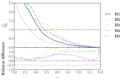
   Figure 1.— Comparison of the number of helium-ionizing photons ($h\nu\geq 54.4$ eV) produced by quasars in each of the simulation models as a function of redshift. Top: the cumulative number of helium-ionizing photons in the simulation volume relative to the number of helium atoms. If all photons produced ionized helium with no recombinations, then helium reionization would be completed by the intersection with this line. Bottom: the number of photons produced relative to Simulation H1. The simulations are described in detail in Section 2.4. Note that Simulation H2 and Simulation H4 in principle produce a comparable number of photons as a function of redshift. Nevertheless, the two simulations have different reionization histories, as well as different reionization topologies.

5. Finally, as a point of comparison, we have run a simulation that does not include explicit quasar sources and instead features a uniform UV background. The photoionization and photoheating rates are given by those in HM12. This allows for a comparison with other studies that employ a uniform UV background (Becker et al., 2011a; Puchwein et al., 2015). However, for a fair comparison with the other simulations presented here, we have renormalized these rates to match $\tau_{\mathrm{eff}}$ as outlined in Section 2.3. Although only the value of $\Gamma_{\mathrm{HI}}$ affects the observed $\tau_{\mathrm{eff}}$, we apply the same renormalization to all of the photoionization and photoheating rates. Simulation H6 uses this uniform background, and can be thought of as the limiting case of having many low-luminosity ($\order{10^{9}-10^{10}\ L_{\odot}}$) objects drive helium reionization, rather than comparatively few high-luminosity ($\order{10^{12}-10^{13}\ L_{\odot}}$) ones.

Figure 1 shows the cumulative number of photons capable of ionizing helium ($h\nu\geq 54.4$ eV) as a function of redshift for each of the simulations presented here. The top panel shows as a point of comparison the total number of helium atoms in the volume. At early times, there are noticeable differences between Simulations H2 and H4, which in principle should both have twice as many photons as Simulation H1. These variations are likely due to shot-noise introduced by the relatively rare quasars, which becomes less extreme at later times. For redshifts $z\lesssim 4$, Simulations H2 and H4 no longer have produced twice as many photons as Simulation H1. This is due to the renormalization process of changing the output of quasars on-the-fly to match $\tau_{\mathrm{HI,eff}}$, as described in Section 2.3. For further details, see Appendix D. If all of the photons produced by quasars were absorbed by helium atoms and there were no recombinations, then helium ii reionization would be completed when equality is reached. Nevertheless, not all photons are absorbed (especially for the highest-energy frequency bin, because of the very low cross-section of helium at these frequencies), and recombination is prevalent, especially in dense regions. Thus, the actual timing of reionization can be significantly different from when photon-helium atom equality is reached.

3. Helium III Ionization Fraction

Figure 2.— Helium ionization fraction $x_{\mathrm{HeIII}}$ as a function of redshift for the different quasar models explored in this work. The top panel shows the ionization fraction, and the bottom panel shows the relative difference compared to the fiducial simulation (H1). The different models presented here are described in Section 2.3 and summarized in Table 1. Among the models shown for comparison is a simulation with a uniform UV background from Haardt & Madau (2012) (Simulation H6). Note that most of the simulations reach a 99% ionization fraction in the range of $2.7\lesssim z\lesssim 3$, which is consistent with observational findings (Dixon & Furlanetto, 2009; Worseck et al., 2011). In all simulations, the duration of helium ii reionization is typically $0.8\lesssim\Delta_{50}\lesssim 1$, with the notable exceptions of Simulations H4 and H6. The durations for these simulations are significantly longer and shorter, respectively, than the other simulations. The former has a long duration due to the early onset of relatively massive quasars, while the latter assumes a quasar emissivity that rises sharply, starting at redshift $z\sim 5$. See the text in Section 3 for additional discussion.

One of the most basic results from the simulations is the calculation of the He iii  ionization fraction as a function of redshift. We define the ionization fraction $x_{\mathrm{HeIII}}$ as the (volume-weighted) amount of doubly ionized helium relative to the total amount for all cells $i$ in the volume:

$$x_{\mathrm{HeIII}}\equiv\sum_{i}\frac{n_{\mathrm{HeIII},i}}{n_{\mathrm{He},i}}.$$ (3)

Given a particular model for the quasar sources, the ionization fraction reflects the impact of these sources on the IGM. For instance, the duration of reionization gives some information about the important sources: a relatively long reionization argues for more sources that are fainter, and a shorter reionization is driven by a few large sources. When comparing features in observables produced from simulations, it is usually more important to compare results at the same ionization fraction than at the same redshift. We refer to different redshifts related to an ionization fraction with a subscript, such that $z_{n}\Rightarrow x_{\mathrm{HeIII}}=n\%$. For instance, $z_{50}\Rightarrow x_{\mathrm{HeIII}}=50\%=0.5$. In addition to finding the redshift corresponding to different ionization fractions, we are also interested in quantifying the duration of reionization. To this end, we define

$$\Delta z_{50}\equiv z_{25}-z_{75},$$ (4)

which corresponds to the duration in redshift of the central 50% change in ionization fraction. We also define a similar quantity $\Delta z_{90}$, which represents the difference between $z_{5}-z_{95}$. We report the redshifts associated with certain ionization fractions, as well as $\Delta z_{50}$ and $\Delta z_{90}$, in Table 1, which summarizes the main results of the simulations. As a reference for converting $\Delta z$ into time units, the shortest reionization scenario, Simulation H6, has a central duration of $\Delta z_{50}=0.58=252$ Myr, whereas the longest reionization scenario, Simulation H4, has a duration of $\Delta z_{50}=1.83=834$ Myr. These reionization scenarios take place over a relatively extended portion of the Universe’s history, and leave a lasting impression on the IGM.

Figure 3.— Comparison of different properties in Simulation H1. Each panel shows a 2-dimensional slice through the simulation volume with the thickness of a single RT cell ($\sim$400 $h^{-1}$kpc). The columns, from left to right, show the He iii  ionization fraction, the gas temperature, the He iii  photoionization rate $\Gamma_{\mathrm{HeIII}}$, and the He iii  photoheating rate $\Lambda_{\mathrm{HeIII}}$. The third and fourth columns only include the contribution to the photoionization and photoheating from the quasar sources, and do not include other sources of ionization and heating (e.g., collisional ionization or heating). The different rows show redshift snapshots corresponding to volume-average ionization fractions of $x_{\mathrm{HeIII}}=0.1,0.25,0.5,0.75,$ and 0.99, from top to bottom. Note that early on in the reionization process, the average He iii  bubble size is small ($\sim$5 $h^{-1}$Mpc), but later on in reionization, the size of ionized regions becomes much larger ($\sim$50 $h^{-1}$Mpc in some cases). This change in bubble size is due to relatively long lifetimes of luminous quasars. The grainy appearance in Columns 3 and 4 is primarily caused by subtle details of the RT implementation and visualization process and is not representative of the accuracy of the calculation.

Figure 4.— Similar plot to Figure 3, but comparing different simulations at redshift $z\sim 3.5$. The rows show from top to bottom Simulations H1, H2, H3, and H4. The value of $x_{\mathrm{HeIII}}$ is shown to the right of each row. In addition to the obvious differences in helium ionization level morphology, the temperature of the IGM (second column) is also very different for the different simulations. There is also an apparent difference between the quasar models used in Simulation H2 (second row) and Simulation H4 (fourth row), which in principle have similar photon counts, but are at different ionization levels. The reasons for these differences are discussed in Section 3.1.

3.1. Ionization Fraction Evolution

Figure 2 shows the volume-averaged ionization fraction of the different simulations as a function of redshift. We define the quantities $\Delta z_{50}$ and $\Delta z_{90}$ as the duration, in redshift, for the volume to transition from 25-75% ionized (by volume) and 5-95% ionized, respectively. In general, helium ii reionization is a very extended process, with $\Delta z_{90}\gtrsim 2$ for almost all of the reionization scenarios, with Simulation H4 having very extended reionization times of $\Delta z_{90}\sim 2.9$. However, there is a large variation in the timing of reionization. The earliest simulation to reach 50% ionization is H4, which occurs at $z_{50}\sim 4.22$. The latest simulation is H3, which occurs at $z_{50}\sim 2.96$. The fiducial reionization scenario, H1, is 50% ionized at $z_{50}\sim 3.34$. As pointed out below in Sections 4 and 5, in general observations are more sensitive to the end of helium reionization, when the volume becomes 90-95% doubly ionized. The main exception to this result is Simulation H2, which reaches a maximum temperature at $z\sim 3.41$, which corresponds to an ionized fraction of 80%. The reason for the difference is related to the method by which the quasar emission is modified to match $\tau_{\mathrm{eff}}$, as outlined in Section 2.3. Nevertheless, knowing the full reionization history has important implications on the thermal history of the IGM.

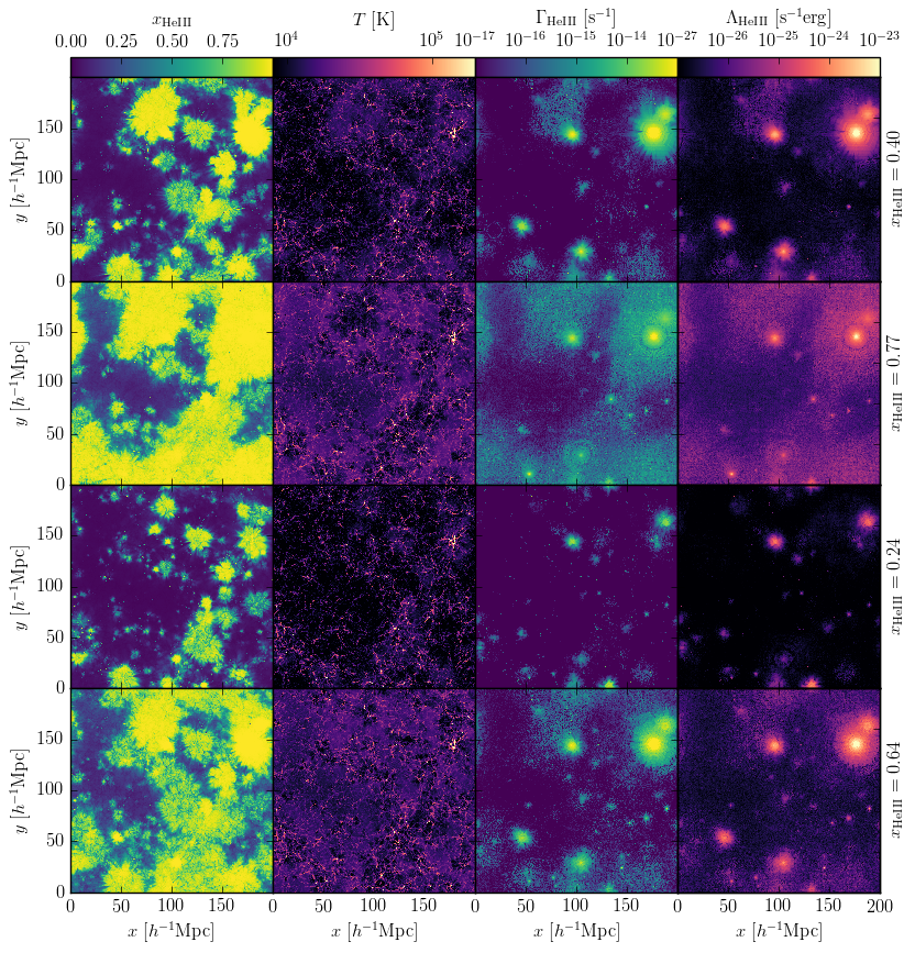
Figure 3 shows visualizations of Simulation H1. The four columns, from left to right, show the He iii  ionization fraction $x_{\mathrm{HeIII}}$, the gas temperature, the He ii  photoionization rate $\Gamma_{\mathrm{HeII}}$, and the He ii  photoheating rate $\Lambda_{\mathrm{HeII}}$. The rows show the same slice of the simulation at increasing values of ionization fraction, which from top to bottom are $x_{\mathrm{HeIII}}=0.1$, 0.25, 0.5, 0.75, and 0.99. The corresponding redshift is shown on the right side of the panels. These slices show a segment of the $yz$-plane of the simulation, with a thickness of one radiative transfer cell in the $x$-direction. This width corresponds to a comoving distance of $\sim$ 400 $h^{-1}$kpc. In a loose sense, the first and second columns are integrated quantities corresponding to the third and fourth columns, respectively. In both cases, the figure shows only photoionization and photoheating rates, which in particular does not include collisional ionization and heating prevalent in regions of high density. Nevertheless, the photoionization and photoheating rates are dominated by the contribution of photons from quasars in the volume. Furthermore, for the temperature of the IGM (Column 2), the hottest regions are found along filaments and other dense regions of cosmic structure. Although these regions are the hottest, photons from quasars dramatically heat the low-density IGM by several thousand kelvin. See Section 4 for further discussion of the IGM temperature.

As discussed in Paper I, in our model the clustering of quasars indirectly affects their lifetimes. Because the lifetimes of quasars affect the size of reionized regions (visible in Figures 3 and 4), the proper clustering affects the coherent scale of reionization. The size of reionized regions also affects the heating of the IGM, as larger reionization regions encompass moderate- to low-density regions earlier than smaller regions. The reason for this is that the relatively fast timing of recombination means that moderate- to high-density gas quickly recombines and requires additional radiation in order to re-reionize. For comparatively large regions, more of the gas that is ionized is low-density, so there is less recombination. Also worth noting is that the relatively high clustering leads to an early overlap of reionized regions, which again reflects the timing of ionization reaching regions of low density.

Figure 4 shows visualizations of Simulations H1, H2, H3, and H4, all at redshift $z\sim 3.5$. Although the underlying gas and large-scale structure is largely similar (as can be seen by comparing Column 2 of the different rows), the ionization and temperature distributions are very different for the different simulations. The differences are driven by the different quasar models used in the simulations. Of particular interest is the difference between Simulations H2 and H4 (Rows 2 and 4). When performing simple photon-counting calculations, as seen in Figure 1, both of these simulations should produce a similar number: Simulation H2 increases by a factor of 2 in the total number of quasars at a given epoch, whereas Simulation H4 increases by a factor of 2 in the number of photons produced per quasar.

Despite this similarity, there are significant differences between the simulations, most notably the ionization fraction (Column 1). Additionally, Columns 3 and 4 show that Simulation H2 has a greater quasar activity at a given redshift. Part of the differences between the simulations can be attributed to the method by which quasars are populated in the volume: as explained in Section 2.1 (and more in depth in Paper I), quasars are placed in halos using abundance matching. Thus, when the amplitude of the luminosity function is increased, sources of the same luminosity are placed in lower-mass halos. In addition to making rare objects more common, there are more sources in general. This feature leads to a greater number of photons intersecting gas cells that have not previously been exposed to quasar radiation.

Figure 5.— Comparison of the gas temperature $T$ as a function of baryon density $\Delta$. The panels are the temperature-density relation as measured from the simulations at $z\sim 2.5$ (top), $z\sim 3$ (bottom left), and $z\sim 3.5$ (bottom right). The gray shaded regions correspond to the 68th and 95th percentiles of Simulation H1. The overall amplitude of the relation rises as redshift decreases, showing that the overall temperature of the IGM increases as helium ii reionization heats up the volume. In addition, the slope of the relation becomes steeper as the simulations evolve. The temperature of relatively dense regions ($\Delta\gtrsim 10$) continues to rise even after helium ii reionization is largely finished. This is due to recombination of the gas, followed by additional reionization, adding more heat to the gas. Conversely, once ionization is completed, the low-density regions ($\Delta<1$) cool adiabatically, with little heat input. The dashed black line in each figure is the best-fit power-law relation given by Equation (5) for Simulation H1. This should be compared with the gray solid line, which follows the relationship for each density value $\Delta$. Note that in general, the simple power law does not accurately capture the relationship between density and temperature. See the text for additional discussion.

Conversely, in Simulation H4, the number of photons produced per source is increased, but the total number of sources is the same as in Simulation H1. (Indeed, the same quasar catalog is used in the two simulations, and only the normalization of quasar radiation is changed between the two. The general morphology of ionized regions in Column 1 and the instantaneous quasar activity in Columns 3 and 4 are very similar in Rows 1 and 4.) Although twice as many photons are produced per source, the long mean free path of helium-reionizing photons means that not all photons are absorbed. Furthermore, as a result of spectral filtering of the radiation from quasars, the photons with energy $h\nu\sim 54.4$ eV will be readily absorbed before more energetic photons, changing the effective SED of the quasar sources (Meiksin et al., 2010). The higher energy photons typically are not absorbed, leading to the large discrepancy in neutral fraction observed between these simulations. Thus, although a simple semi-analytic calculation would yield the same reionization time for these two simulations, we can see that a full treatment leads to important differences between the two cases.

The ionization fraction observed in our simulations is worth comparing with the results of McQuinn et al. (2009) and Compostella et al. (2013), hereafter M09 and C13. The duration of reionization in our simulations is comparable to the models explored in M09 (as seen in their Figure 3). However, the reionization histories in C13 are much briefer than those seen here. This is largely because the quasar population in their fiducial reionization model does not include sources for $z>4$. The authors include an additional “extended” model that includes sources beginning at $z=5$, which shows a duration of reionization more comparable to those in M09 and this work. Observations from McGreer et al. (2013) show a non-negligible population of high-redshift quasars, which in Simulation H1 causes the ionization fraction of helium to have a value of a few percent at $z\sim 5$, with the volume being nearly a quarter ionized by $z\sim 4$. Thus, future studies should include high-redshift quasars as an important part of helium ii reionization.

4. The Temperature History of the IGM

One important impact of helium ii reionization on the IGM is the temperature feedback. Since quasars emit a hard spectrum with many energetic photons and the IGM is in a highly ionized state, the excess energy remaining after photoionization is converted into heat in the gas. Although secondary ionizations are possible (e.g., Shull 1979; Furlanetto & Stoever 2010), their impact is negligible for helium reionization because of the ionization level of the IGM (McQuinn et al., 2009). Photoheating from radiation from quasars increases the average temperature of the IGM by $\sim$10,000 K, and as we show in Sections 4.1 and 4.2, contains important information about the history of helium ii reionization.

4.1. Temperature-Density relation

The relationship between the temperature of the IGM $T$ and the baryon overdensity $\Delta\equiv\Delta_{b}$ is an important measure of the state of the IGM, and it is intimately related to the reionization process. One can write the relationship between temperature and density as a power law and fit for the two parameters that define it (Hui & Gnedin, 1997):

$$T(\Delta)=T_{0}\Delta^{\gamma-1},$$ (5)

where $T$ is the gas temperature, and $T_{0}$ and $\gamma$ define the power-law relation between the gas density and temperature. This is the so-called temperature-density relation, also sometimes called the equation of state of the IGM (although we note that it is not a true equation of state). Hui & Gnedin (1997) showed that at late times following hydrogen reionization, the slope of the relation approaches $\gamma=1.62$. In general, this relationship should hold for the low-density gas in the IGM where adiabatic cooling or heating and a uniform radiation field following reionization are the dominant sources of temperature change. However, the addition of heat from helium ii reionization changes the slope of this relation, as well as the overall amplitude.

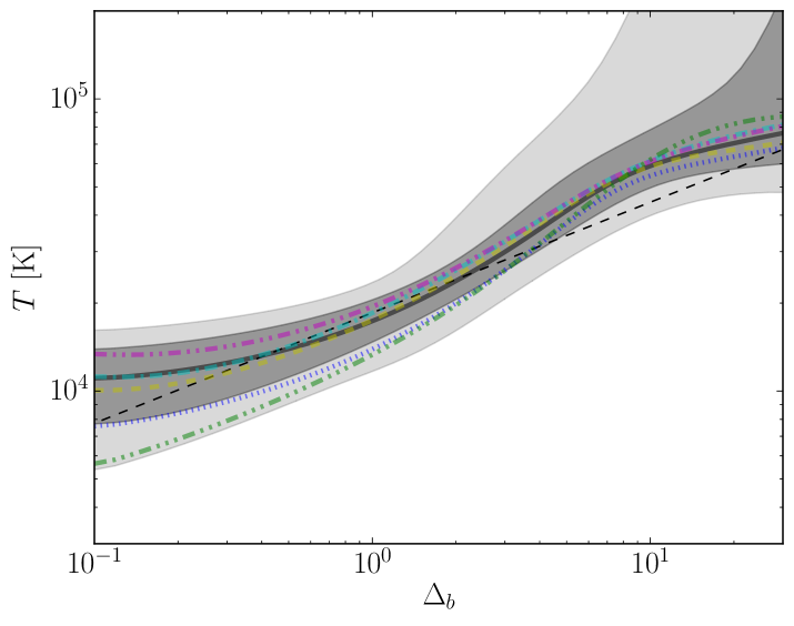
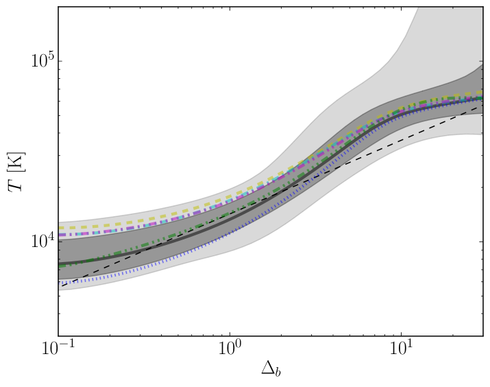
Figure 5 shows the temperature-density relation for the gas in the different simulations. The relationship is shown at several different redshifts, in order to demonstrate several different effects that reionization has on the IGM temperature. In particular, the general trend is indicative of an “inside-out” reionization scenario. In such a scenario, the radiation from sources (quasars, in this case) propagate outward, and are absorbed in high-density regions near sources before low-density ones, depositing heat as the radiation is absorbed. Because the gas is reionized at different times and is dominated by adiabatic cooling following reionization, the relative temperature between different gas densities reflects the reionization history. In particular, the temperature of underdense regions can in fact be higher than mean-density regions because the radiation from quasars tends to reach these regions at a later redshift. In the meantime, the gas from high-density regions has additional time to cool adiabatically. Because the amount of heat deposited in the gas from photoionization does not depend on the density, the gas from higher density regions may be at a lower temperature than the low-density gas when the low-density gas is reionized. Thus, the temperature-density relation can be relatively flat for medium- to low-density gas, and even turn over such that low-density regions have a higher temperature than mean-density ones (e.g., as in Trac et al. 2008 for hydrogen reionization). The simulations presented here do not exhibit this inversion because of both the longer mean free path of helium-ionizing photons and the relatively smaller amount of adiabatic cooling experienced by gas at this redshift. Nevertheless, several of our simulations, and Simulation H5 at $z\sim 3$ in particular, show a relatively flat relation for underdense regions.

Another feature in Figure 5 is the evolution of regions of high density ($\Delta\gtrsim 10$). In these regions, the density of gas is high enough that an appreciable fraction of the doubly ionized helium can recombine with electrons to form singly ionized helium. Once the gas has recombined, it can undergo an additional reionization event, which will deposit additional heat into the gas. As can be seen in the Figure, the higher density regions show higher temperatures as redshift decreases, even after helium ii reionization is nominally completed. Thus, the temperature of these different regions at the same redshift can somewhat break the degeneracy between the different reionization scenarios. Since these differences are visible in higher density gas, it may be possible to observe these differences in the Ly$\beta$ forest, since these observations saturate at higher densities than Ly$\alpha$ (Dijkstra et al., 2004; Iršič & Viel, 2014).

Figure 6.— Parameters of the IGM power law temperature-density relation in Equation (5) as a function of redshift for the different simulations. The top panel shows the temperature parameter $T_{0}$, and the bottom panel shows $\gamma$. In the panel for $\gamma$, we have shown the line of $\gamma=1.62$, the predicted slope from Hui & Gnedin (1997) for the relation following hydrogen reionization. At early times, Simulation H6 approaches this value, but then deviates from it following helium reionization. The other simulations do not approach this value, probably because helium ii reionization begins before a steady state can be established. As discussed in the text, the initial flattening of the slope ($\gamma<1.6$) is due to the inside-out nature of reionization, and the later steepening ($\gamma\sim 1.62$) is due to establishing equilibrium with the radiation field. For the $T_{0}$ parameter, the rise and fall of the value is consistent with the rise and fall seen in Figure 5. See the text for further discussion.

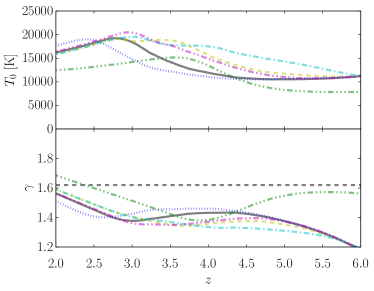
Figure 6 shows the evolution of the parameters of the temperature-density relation given in Equation (5) as a function of redshift for the different simulations. We find a linear fit for the parameters after applying a log-transform to the temperature and density for each gas cell, and volume-weight the results. As can be seen by the general structure of Figure 5 and as was noted in C13, fitting the entire temperature-density relation to a single power law may not be the optimal parameterization because of the wide dispersion of temperatures at a given density value. We should note that part of the difficulty in fitting the result to a power law comes from the approximate nature of the relation: for high values of $\Delta$, the approximation breaks down. Furthermore, the resolution of the simulations does not capture all of the structure of the IGM, which leads to smoothing at certain scales. Nevertheless, we present these results for the sake of comparison.

In general, we see a similar trend to Figure 5, where the temperature value at mean density $T_{0}$ increases as reionization proceeds, reaches a peak value, and then decreases again. This is a general trend seen in the thermal evolution of the IGM and is explored more below in Section 4.2. Another general trend is the evolution of the power-law index $\gamma$ which is roughly consistent between simulations. We reproduce the observation of M09 that $\gamma\sim 1.3$ during the bulk of helium reionization for our different scenarios. In the lower panel of Figure 6 we show the value of $\gamma=1.62$, which is the asymptotic value of the IGM from Hui & Gnedin (1997) following hydrogen reionization without additional sources of photoheating.

As can be seen from Figure 6, simulations that include a patchy hydrogen reionization are not consistent with this value, although Simulation H6, which features a significantly earlier hydrogen reionization epoch, approaches this value. However, once helium ii reionization begins, there is a notable flattening of the temperature-density relation (where $\gamma=1$ represents the limit of an isothermal gas). As a larger portion of the volume becomes ionized, denser regions will recombine and undergo additional reionization events, leading to additional heat being deposited at these densities. Conversely, low-density regions are dominated by adiabatic cooling. This leads to an overall steepening of the slope $\gamma$, a trend seen at low redshifts following the completion of helium ii reionization. These trends are also visible in Figure 5. In particular at $z\sim 3$, most of the simulations have a comparable value of $\gamma$. Indeed, the shape of these temperature-density relations in the central panel of Figure 5 is similar, albeit with different vertical offsets.

The results of M09 and C13 are largely consistent with the findings presented here. Before helium ii reionization begins, the temperature-density relation tightly follows a power-law expression. Once helium ii reionization begins, the distribution of temperature as a function of density becomes highly variable, with a large dispersion forming for a given density value. This dispersion signifies the inhomogeneous reionization process and is a general feature of helium ii reionization. Additionally, as in C13, we find that the overall relation between temperature and density is ill-fit by a single power law. C13 finds that the temperature-density relation flattens out and begins to turn over at $\Delta\sim 10$ (cf. their Figure 8). Although we do not see a turn-over in our measurements, it is still clear that using a single power law to characterize the relationship between temperature and density is insufficient for the IGM following reionization.

4.2. Temperature at mean density

Figure 7.— Median temperature at mean density ($0.95\leq\Delta\leq 1.05$) of the IGM as a function of redshift. The temperature at mean density is significantly higher for the patchy hydrogen reionization scenarios than for the one with a uniform UVB (Simulation H6), because the hydrogen reionization occurs significantly earlier. Once quasar activity begins, the temperature of the IGM rises as a result of photoheating. The peak corresponds to an ionization fraction of $x_{\mathrm{HeIII}}\sim 0.90$-0.95, marking the tail-end of reionization. Following helium ii reionization, the mean-density gas begins to adiabatically cool again, leading to the peak structure seen in the Figure. See the text for additional discussion.

An important marker of the progress of helium ii reionization is the temperature at mean density of the simulation ($\Delta\sim 1$), since the temperature in these regions is dominated by adiabatic cooling of the Universe and heating from radiative transfer (Hui & Gnedin, 1997). The interplay of these two factors determines the temperature of these regions of average density. The average temperature of these regions show two characteristic bumps as a function of redshift: one initial increase from $T\sim 200$ K to $T\sim 10^{4}$ K as a result of hydrogen reionization at $8\lesssim z\lesssim 10$, and a subsequent increase in temperature from $T\sim 10^{4}$ K to $T\sim 2\times 10^{4}$ K at $2\lesssim z\lesssim 3.5$ as a result of helium reionization (Furlanetto & Oh, 2008; Puchwein et al., 2015; Upton Sanderbeck et al., 2016). In between the two epochs of reionization, and following helium ii reionization, adiabatic cooling dominates, and so the average temperature decreases. The locations and widths of these features can provide valuable insight into the timing and duration of reionization.

Previous studies of the mean temperature of the IGM, both semi-analytic (Furlanetto & Oh, 2008) and using simulations with a uniform UVB (Puchwein et al., 2015; Bolton et al., 2016) have shown that the general picture of the IGM temperature should hold, and it can therefore be used to extract information about reionization. For our purposes here, we concern ourselves primarily with this second epoch of heating in the IGM, corresponding to helium ii reionization.

Figure 8.— Visualization of two typical sightlines through the simulation volume at $z\sim 2.7$. The sightlines shown in each figure are taken from the same physical location in the volume from all simulations and therefore encounter similar large-scale structure. The segments shown here are about 10 comoving $h^{-1}$ Mpc in size. The differences in flux between simulations can be significant, although not always in the same direction. This behavior argues for calculating flux explicitly using Equation 6 rather than using an approximate expression for $\tau$. Relatively large differences in regions of low flux ($F\lesssim 0.1$) are due more to the low values of flux than to significant differences between the simulations. See the text in Section 5 for further discussion.

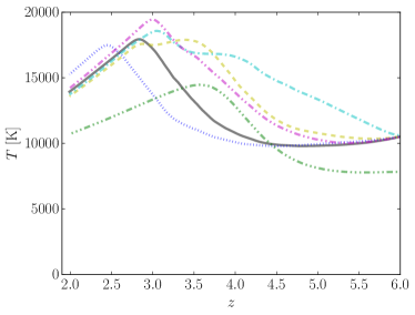
Figure 7 shows the median temperature at mean density of the different simulations. In order to compute the temperature at mean density, at each time step in the simulation we find the median temperature (as well as the $\pm$68th and 95th percentiles) of all gas cells that have $0.95\leq\Delta\leq 1.05$. At high redshift ($z\gtrsim 6$), the simulations have largely the same temperature because the IGM temperature is dominated by hydrogen reionization. As explained in Section 2.3, all of the simulations with explicit quasar sources use a semi-analytic method for calculating patchy hydrogen reionization. The exception to this is Simulation H6, which uses the uniform UV background of HM12 for both hydrogen and helium reionization. Notably, the timing of hydrogen reionization is significantly earlier than for the patch hydrogen method used ($z_{\mathrm{re}}\sim 13$ for HM12 compared to $z_{\mathrm{re}}\sim 8$ for the patchy hydrogen), so the IGM has had additional time to adiabatically cool. This leads to the lower initial temperature at $z\sim 6$ seen in Figure 7.

We also note that in Figure 7 the temperature of the IGM peaks at a redshift that corresponds to 90-95% of the helium iii ionization level. This is consistent with the idea that the gas at mean density composes a large fraction of the volume of the simulation volume and so will preferentially reionize later than regions of high density. Following this peak in the IGM temperature, the adiabatic cooling of the Universe becomes the dominant mechanism because this comparatively low-density gas generally does not recombine (because recombination is $\propto\rho_{g}^{2}$, as shown in Equation (2)).

5. Measurements of the Ly$\alpha$ Forest

An important observational tool used to understand helium ii reionization is the Ly$\alpha$ forest. Observationally, there have been many rich data sets using the Ly$\alpha$ forest, especially for cosmological measurements. The BOSS sample (Lee et al., 2013) has been used to observe the baryon acoustic oscillation (BAO) feature (Busca et al., 2013; Slosar et al., 2013), as well as generate one-dimensional power spectra (Palanque-Delabrouille et al., 2013), which have been used to constrain neutrino masses and other cosmological parameters (Palanque-Delabrouille et al., 2015). High-resolution measurements from Keck-HIRES and Magellan-MIKE (Lu et al., 1996; Becker et al., 2007, 2011b; Calverley et al., 2011) have given us information about the temperature history of the IGM.

Synthetic Ly$\alpha$ spectra can be created for the H i  and He ii  densities. (See Paper III of this series for further discussion of the He ii  Ly$\alpha$ forest). In the following analysis, we have drawn the spectra along the $x$-axis of the simulation, although we find nearly identical results when projecting along different axes. Once these spectra have been calculated, they can be used to measure the effective optical depth $\tau_{\mathrm{eff}}$ of the volume, compute the flux PDF, and calculate one-dimensional power spectra. To generate a synthetic sightline, we define a set of pixels along a line of sight in the simulation volume, such that the number of pixels is equal to the number of grid cells. For the resolution level discussed in these simulations, this means $N_{\mathrm{pix}}=2048$. The resulting resolution of the Ly$\alpha$ forest is about 98 kpc $h^{-1}$ comoving. Lukić et al. (2015) showed that at a comparatively high-redshift ($z\gtrsim 3.5$) resolution of $\sim 20$ kpc $h^{-1}$ comoving was required to resolve all features of the Ly$\alpha$ forest to sub-percent level accuracy, especially at small scales. Thus, some inaccuracies may be introduced at small scales and high redshift from the resolution of the simulations. At the same time, at mean density at $z\sim 3$ the Jeans scale is typically 500 kpc $h^{-1}$ comoving, so the simulation has sufficient resolution to capture features introduced by Jeans smoothing.

For each pixel $i$, the optical depth of the pixel $\tau_{i}$ is calculated through the contributions of every other pixel according to the formula (Bolton et al., 2009b)

$$\tau_{i}=\frac{c\sigma_{\alpha}\differential{R}}{\pi^{1/2}}\sum_{j=1}^{N_{\mathrm{pix}}}\frac{n_{\mathrm{HI}}(j)}{b_{\mathrm{HI}}(j)}H(a,x),$$ (6)

where $\sigma_{\alpha}=4.479\times 10^{-18}$ cm^-2 is the cross-section of the Ly$\alpha$ transition, $b_{\mathrm{HI}}=\sqrt{2k_{B}T/m_{\mathrm{H}}}$ is the Doppler parameter, $\differential{R}$ is the (physical) width of the pixel, and $H(a,x)$ is the Voigt-Hjerting function (Hjerting, 1938):

$$H(a,x)=\frac{a}{\pi}\int_{-\infty}^{\infty}\frac{e^{-y^{2}}}{a^{2}+(x-y)^{2}}\differential{y},$$ (7)

where $x=[v_{\mathrm{H}}(i)-u(j)]/b_{\mathrm{HI}}(j)$ is the difference in redshift space between pixels $i$ and $j$ relative to the Doppler broadening, $u(j)=v_{\mathrm{H}}(j)+v_{\mathrm{pec}}(j)$ is the total velocity difference of Hubble flow plus peculiar velocity, $a=\Lambda_{\alpha}\lambda_{\alpha}/4\pi b_{\mathrm{HI}}(j)$ represents the gas damping, where $\Lambda_{\alpha}=6.265\times 10^{8}$ s^-1 is the damping constant and $\lambda_{\alpha}=1215.67$ Å is the wavelength corresponding to the Ly$\alpha$ transition. In order to efficiently compute the Voigt-Hjerting function, we use the analytic approximation provided by Tepper-García (2006).

As can be seen from Equations (6-7), the thermal properties of the gas enter in the form of the Doppler parameter $b$. This term increases as the temperature of the gas increases and serves to broaden the apparent width in velocity space of a particular gas parcel. The tendency of absorption features to widen in velocity space as the temperature increases can be used to learn about the thermal state of the IGM. More approximately, the local optical depth of the IGM will depend on the average temperature of the volume. We will further discuss some of the implications of this process below in Section 5.2. The temperature of the gas can also affect the hydrogen ionization level, since the recombination coefficient $\alpha_{\mathrm{HII}}$ in Equation (2) decreases with increased temperature.

Figure 8 shows two typical sightline sections generated from the gas properties in the simulations at $z\sim 2.7$. These synthetic spectra have a comoving size of about 10 $h^{-1}$ Mpc. The sightlines in different simulations are drawn from the same location in the simulation volume, which means that the sightlines encounter similar large-scale structure of the underlying gas. Accordingly, the differences in flux observed can be traced to local differences in the radiation field.

As described in Section 2.3, all of the simulations have been renormalized such that the overall effective optical depth $\tau_{\mathrm{eff}}$ is consistent across simulations. This allows for more straightforward comparison between simulations. It also allows for us to determine which statistical differences observed in the simulations can be attributed to the timing of helium ii reionization.

We note that the general large-scale absorption is similar across simulations. Also worth mentioning is the fact that differences between simulations are not always in the same direction. For instance, in the bottom panel of Figure 8, Simulation H5 shows higher flux than Simulation H1 in an absorption feature at $v\sim 250$ km s^-1, and more absorption at $v\sim 800$ km s^-1. These differences are due to relatively small-scale effects of being nearby quasars that are active at different times in some simulations, or perhaps not at all in others. There are also relatively large differences in regions of low flux. These differences are driven primarily by there being little overall flux, rather than truly having large deviations between simulations.

5.1. Effective Optical Depth

Once the optical depth for each pixel has been calculated, the corresponding flux is given simply by $F_{i}=\exp(-\tau_{i})$. We can then define the effective optical depth of the volume by averaging over all values of the flux:

$$\expectationvalue{F}=\exp(-\tau_{\mathrm{eff}}).$$ (8)

In general $\tau_{\mathrm{eff}}\neq\expectationvalue{\tau}$. The effective optical depth as a function of redshift has been measured to high precision as a volume-averaged quantity for the H i  forest (Lee et al., 2015) and for individual objects of the He ii  forest (Worseck et al., 2014). Lee et al. (2015) reported that the BOSS survey measures more than 50,000 quasar spectra at intermediate-to-high redshift and has a formula for the evolution of the effective optical depth as a function of redshift $\tau_{\mathrm{eff}}(z)$.

In general, cosmological simulations of the Ly$\alpha$ forest must renormalize the flux level measured in order to match the observed optical depth measurements (see, e.g., Bolton et al. 2009b). The reason is that the resolution of these simulations is typically not high enough to capture the small-scale high-absorption LLSs and damped Ly$\alpha$ systems that can lead to cosmological simulations predicting too high of a value of $\tau_{\mathrm{eff}}$ (although see McQuinn et al. 2009 for attempts to account for these systems in simulations). Typically, this renormalization of Ly$\alpha$ spectra is done in post-processing when the sightlines are generated.

Figure 9.— Effective optical depth of hydrogen $\tau_{\mathrm{eff,HI}}$ as a function of redshift for the different simulations. The solid black line shows the observational data from Lee et al. (2015). The line styles for the simulations are the same as in Figure 2. As discussed in Section 5.1, the amount of hydrogen-ionizing radiation from galaxies $\Gamma_{\mathrm{gal}}$ is modified while the simulation is running, so that this quantity is matched by construction. This avoids the requirement of renormalizing the simulations in post-processing.

Figure 10.— Comparison of the flux PDF of the H i  Ly$\alpha$ forest at $z\sim 2.5$ (top),$z\sim 3$ (bottom left), and $z\sim 3.5$ (bottom right). All of the simulations have the same color scheme as in Figure 2. In the bottom left panel, the data points are taken from the results of Calura et al. (2012), at $z\sim 2.9$. All of the simulations show a generally similar distribution of fluxes. This result implies that the flux PDF is only weakly sensitive to the temperature information of the IGM, since the only main difference between the simulations (except for the helium ionization fraction) is the temperature. The flux PDF is instead more sensitive to $\tau_{\mathrm{eff}}$ and observationally, to the continuum-level uncertainty of the Ly$\alpha$ forest. See the text in Section 5.2 and Appendix B for additional details.

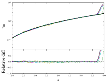
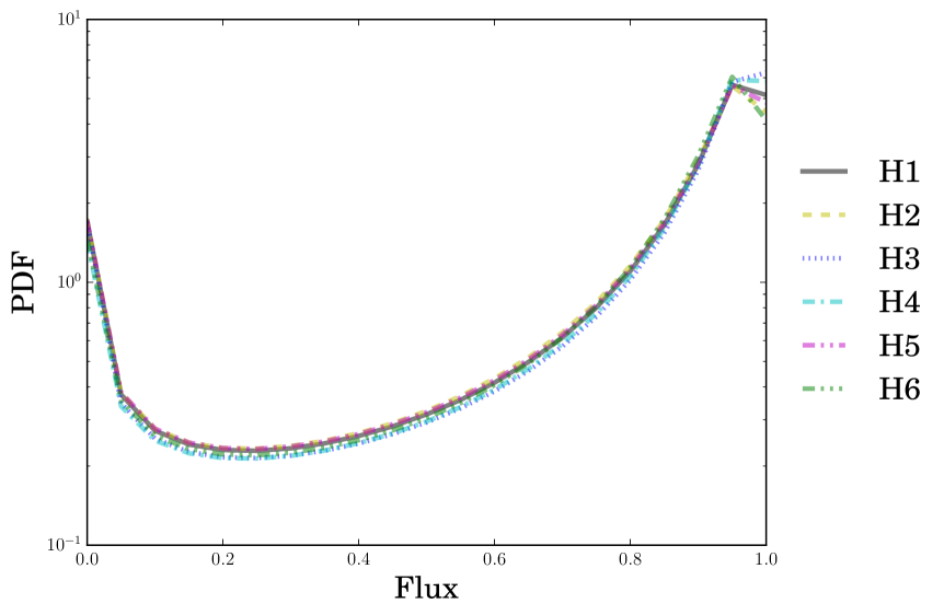
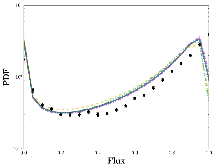
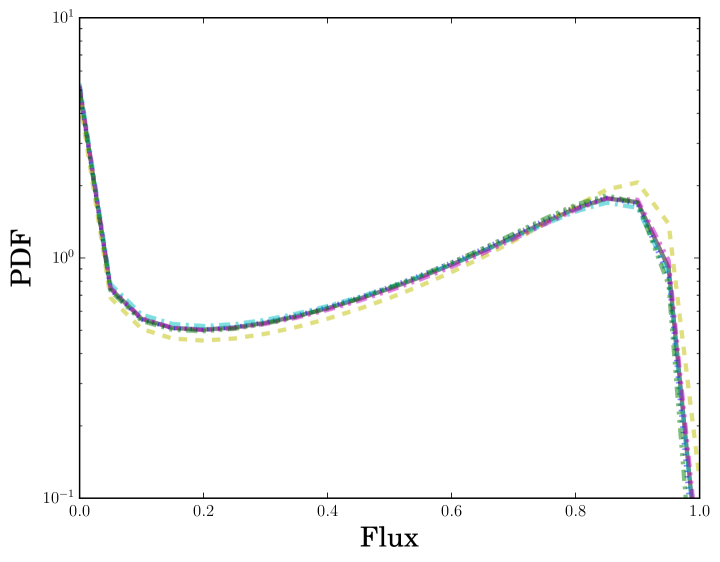
Figure 9 shows $\tau_{\mathrm{eff}}$ for all of the simulations presented in this work. As noted in Section 2.3, this quantity is matched by construction for all of the simulations. In general the agreement is excellent. For redshifts $z\lesssim 6$ (the nominal end of hydrogen reionization, after which $\tau\lesssim 1$), all of the simulations match the observed value from Lee et al. (2015) to within a few percent. This matching allows for a more straightforward comparison between the simulations and observations.

As explained in Sections 2.3 and 2.4, our simulations change the value of $\Gamma_{\mathrm{gal}}$ on-the-fly in order to match the value of $\tau_{\mathrm{eff}}$ as specified by Lee et al. (2015). By ensuring that all of our simulations match the same value of $\tau_{\mathrm{eff}}$, we are better able to compare them with each other and with the observations. Previous studies of the Ly$\alpha$ forest (Theuns et al., 2002; Ciardi et al., 2003; Dall’Aglio et al., 2008; Faucher-Giguère et al., 2008b) have reported a dip in $\tau_{\mathrm{eff}}$ at $z\sim 3.2$. In some of these works, the authors cited this dip as evidence of helium ii reionization because an increased IGM temperature decreases the optical depth. By matching the $\tau_{\mathrm{eff}}$ of Lee et al. (2015), which does not contain this dip, it is possible that we would miss this feature. We explore this possibility in more detail in Appendix A.

When we compare our results with the simulations of M09 and C13, in all cases, $\tau_{\mathrm{eff}}$ is comparable to the most recent determinations of the H i  Ly$\alpha$ forest for the then state-of-the-art measurements. Our simulations are the only ones that renormalize $\Gamma_{\mathrm{HI}}$ in real time, so we are able to match the value of $\tau_{\mathrm{eff}}$ by construction. Nevertheless, our values of $\Gamma_{\mathrm{HI}}$ are comparable to those in M09 and C12, as well as HM12. We again note that the relative uncertainty on $\Gamma_{\mathrm{HI}}$ is much larger than that of $\tau_{\mathrm{HI}}$, and so to generate more realistic comparisons with measurements of the H i  forest, we advocate matching the value of $\tau_{\mathrm{eff}}$ by construction, as we have done here.

5.2. Flux PDF

Another statistic related to the Ly$\alpha$ forest is the flux PDF. This measurement is carried out by taking the flux value of each of the pixels in the sightlines of the Ly$\alpha$ forest and creating a normalized PDF of their values. The result gives additional information about the distribution of gas in the IGM. The flux PDF is also dependent on the resolution of the measurement. For instance, compare the results from a relatively high-resolution measurement (Calura et al., 2012) with that of a relatively low-resolution measurement (Lee et al., 2015). In the lower resolution case, the pixels of extreme absorption or emission become averaged, and the flux PDF tends toward the mean. Thus, the measured PDF is resolution dependent.

Figure 11.— Same plots as in Figure 10, but with binning performed at higher resolution. The redshifts chosen are $z\sim 2.5$ (top), $z\sim 3$ (bottom left), and $z\sim 3.5$ (bottom right), the same as in the previous figure. In addition, only flux values of $0.6\leq F\leq 1.0$ are plotted to emphasize the most different portions of the flux PDF. The flux PDF shows a much more gradual transition at $F\sim 1$ than the PDF conveyed in Figure 10, further emphasizing that the resolution and binning of the flux PDF are important for understanding it. The higher resolution also makes the differences between simulations more apparent, especially at $z\sim 3$.

From a simulation point of view, the resolution of the gas grid (and to a lesser extent, the radiation grid) affects the resolution of the Ly$\alpha$ forest. For the default-resolution grid at $z\sim 3$, a single gas cell has an equivalent velocity width of $\Delta v=7.3$ km s^-1. This resolution level is significantly greater than that of BOSS ($\Delta v\sim 69$ km s^-1, Lee et al. 2015), though not as good as Keck-HIRES ($\Delta v\sim 6.6$ km s^-1, Lu et al. 1996).

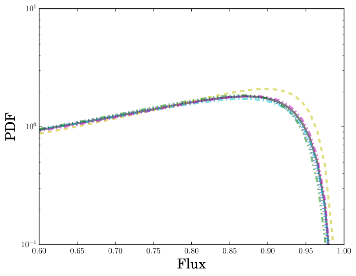
Figure 10 shows the flux PDF of the H i  Ly$\alpha$ forest as a function of redshift across the various simulations. The figure also includes the measurements of Calura et al. (2012). The spectra from Calura et al. (2012) were taken at UVES, with a FWHM of 6.7 km s^-1, slightly better than the resolution of our simulations. As a result, the different resolution may have a non-trivial impact on the shape of the resulting flux PDF. The flux PDF in general has a similar shape for different simulations at the same redshift although the simulations have different He iii  ionization fractions and thermal histories. This result implies that given the same underlying gas structure, the flux PDF depends on having the same value of $\tau_{\mathrm{eff}}$. Given the same large-scale structure and $\tau_{\mathrm{eff}}$, our result shows that helium reionization is largely undetectable in the hydrogen flux PDF.

Nevertheless, there are still several trends that are visible upon closer inspection. After helium reionization is largely completed at $z\sim 2.5$, the values of the flux PDF in the highest transmission bin of $F\sim 1$ are ordered by the helium ionization fraction: Simulation H3 has the highest value in this bin, and Simulation H6 has the lowest. Helium ii reionization is still ongoing for Simulation H3, whereas for the other simulations, reionization is largely completed (Figure 2).

We can understand this trend by employing the fluctuating Gunn-Peterson approximation (FGPA, Croft et al. 1998). The FGPA assumes that the gas of the IGM accurately follows a temperature-density relation of the form found in Equation (5) and is in photoionization equilibrium with a uniform ionization background. Under these assumptions, the local optical depth of the IGM $\tau_{\mathrm{HI}}$ can be expressed in terms of the gas density, mean temperature of the IGM, and the H i  photoionization rate, along with other cosmological parameters. In particular, it can be shown that the optical depth is related to the temperature as $\tau_{\mathrm{HI}}\propto T^{-0.7}$. Thus, for reionization histories with a higher average temperature, there is a decreased local value of $\tau$, leading to an overall higher flux value everywhere, but in low-density regions in particular. Therefore, the comparatively high value for the flux PDF in the bin where $F\sim 1$ for Simulation H3 can be interpreted as conveying information about the thermal state of the IGM. Indeed, Lee et al. (2015) have proposed using the flux PDF to gain information about the thermal state of the IGM at different redshifts.

One point to note is the visible difference between the observations of Calura et al. (2012) at $z\sim 2.9$ and the results from the simulations at $z\sim 3$, shown in the bottom left panel in the plot. The flux PDF at intermediate flux values in the simulations is higher than that of the observations, until the highest bin (where there is almost total flux transmission). Part of the difference can be attributed to the fact that the simulations and the observations are normalized to different values of $\tau_{\mathrm{eff}}$: the simulations use the value from Lee et al. (2015), whereas the observational results determine the parameters for $\tau_{\mathrm{eff}}(z)$ based on their measurements. At $z\sim 3$, the results for $\tau_{\mathrm{eff}}$ from Lee et al. (2015) are higher than those from Calura et al. (2012) by about 30%. This result accounts for some of the difference in the flux PDF, but not all of it. (See Appendix B for further discussion of the renormalization effect.) Alternatively, as discussed in Calura et al. (2012), the continuum-level estimation of the observational Ly$\alpha$ forest can significantly affect the shape of the flux PDF. As shown in Figure 8 of Calura et al. (2012), increasing the continuum level by 5% modifies the shape of the flux PDF to be comparable to the levels seen in the simulations. Thus, a combination of changing $\tau_{\mathrm{eff}}$ of the simulations and the continuum-level of the observations can bring the simulations and observations into agreement.

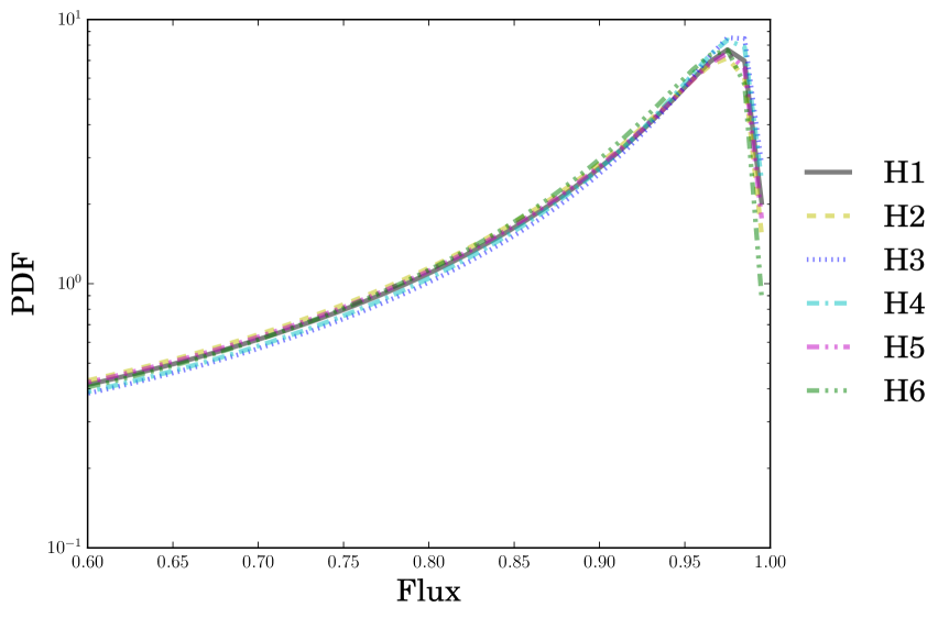
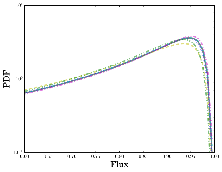
Figure 11 shows the flux PDF for the simulations, but binned at higher resolution than in Figure 10. The increased resolution in the binning shows a much more gradual transition at $F\sim 1$ than the stark fall-off in Figure 10. This higher-resolution binning also clarifies the differences between the simulations. As mentioned above, these differences are likely due to the thermal state of the IGM, since in the FGPA the absorption is proportional to the temperature. High-resolution measurements of the flux PDF may therefore yield information about the thermal state of the IGM, although as discussed in Appendix B, the determination of the continuum-level flux for observations remains a significant systematic uncertainty. The continuum level plays a significant role here as well, since it determines the distribution of $Fsim1$ pixels when generating a PDF.

5.3. One-dimensional flux power spectra

Figure 12.— One-dimensional flux power spectrum of the H i  Ly$\alpha$ forest at $z\sim 2.5$ (top), $z\sim 3$ (bottom left), and $z\sim 3.5$ (bottom right). Black dots with error bars are observational data measured from BOSS as reported by Palanque-Delabrouille et al. (2013) as reported at $z\sim 2.4$, $z\sim 3$, and $z\sim 3.4$, respectively. In general, the data points agree with the simulations, although this agreement at these scales is likely due primarily to having comparable values of $\tau_{\mathrm{eff}}$. The effects of helium ii reionization are visible in the small-scale power. Specifically, simulations in which the average temperature of the IGM is higher show lower power on small scales. This is due to the thermal motion of the gas, which washes out some of the small-scale structure. The overall amplitude of the power spectrum tends to decrease with redshift, since the total number density of hydrogen is decreasing. See the text for additional discussion.

In addition to the statistics already discussed, the one-dimensional flux power spectrum can provide valuable information about underlying dark matter density distributions. To calculate the one-dimensional flux power spectrum, we first define a “flux overdensity” $\delta_{F}$ for each pixel:

$$\delta_{F}\equiv\frac{F}{\expectationvalue{F}}-1,$$ (9)

where $\expectationvalue{F}$ is the average flux for all pixels in the volume (which is also typically close to the average flux within a given sightline because of the length of the sightlines). After defining this quantity, a Fourier transform is applied to each sightline, so that we have $\delta_{F}(k)$. The one-dimensional power spectrum $P_{\mathrm{1D}}(k)$ is the average power per $k$-mode: $P_{\mathrm{1D}}(k)=\expectationvalue*{\absolutevalue{\delta_{F}(k)}^{2}}$. In the following analysis, we primarily study the dimensionless power spectrum,

$$\Delta^{2}_{\mathrm{1D}}(k)=\frac{k}{\pi}P_{\mathrm{1D}}(k).$$ (10)

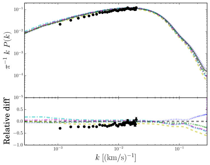
Previous studies have shown that the one-dimensional power spectrum can be used to measure the three-dimensional power spectrum (Croft et al., 1998; McDonald et al., 2005; McDonald & Eisenstein, 2007), although here we explore the one-dimensional power spectrum per se and treat the three-dimensional power spectrum separately in Section 5.4. As with the flux PDF, the amplitude of the one-dimensional power spectrum on large scales is largely similar between the different reionization scenarios at the same redshift. However, there are significant differences on small scales ($k\gtrsim 0.1\ (\mathrm{km/s})^{-1}$). This is likely due to the differences in the thermal histories of the IGM. In particular at $z\sim 2.5$, Simulation H6 shows a greater amplitude than many of the other simulations and also has a cooler temperature (see Figure 7). The cooler temperature is correlated with additional power at small scales, which is consistent with additional structure as a result of cooler gas.

Figure 12 shows the one-dimensional power spectrum of the Ly$\alpha$ forest for redshifts $z\sim 2.5$, $z\sim 3$, and $z\sim 3.5$. As with the flux PDF in Figure 10, the simulations show largely similar result. Nevertheless, key differences due to the effects of helium ii reionization are still visible. Most of the differences between simulations are visible at small scales. In general, the simulations that have a hotter average temperature of the IGM show less power at small scales. This is due to the decrease in clumping that results from the increased thermal motion of the gas. On large scales, the differences between the simulations are typically smaller than 10%.

The data points in Figure 12 are the results from Palanque-Delabrouille et al. (2013) from BOSS. The data plotted show redshift values of $z\sim 2.4$, $z\sim 3$, and $z\sim 3.4$, compared to the redshift values of $z\sim 2.5$, $z\sim 3$, and $z\sim 3.5$ from the simulations. The slight discrepancy in redshift for the plots may lead to some of the differences seen, especially for the plot from the simulations at $z\sim 3.5$. Nevertheless, there is good agreement in general between the data and the simulations. A primary driver of this agreement may be the similar values of $\tau_{\mathrm{eff}}$ in the data and simulations. The value of $\tau_{\mathrm{eff}}$ in the simulations matches that of Lee et al. (2015) is based on SDSS DR7 data, whereas the results from Palanque-Delabrouille et al. (2013) include additional data from BOSS. On the scales where the data are reported, the difference between the different simulations is small. As such, the data are not able to break the degeneracy between the simulations.

Figure 13.— Three-dimensional power spectrum of the H i  Ly$\alpha$ forest flux at $z\sim 2.5$ (top), $z\sim 3$ (bottom left), and $z\sim 3.5$ (bottom right). The most significant differences between the simulations emerge on large scales. In previous studies on the three-dimensional power spectrum (McDonald, 2003), the deviations due to different thermal histories of the IGM led to differences of $\sim 10\%$, consistent with the results presented here. The dramatic differences on large scales may be due to correlations in the radiation field that are the result of quasar emission. See the discussion in Section 5.4 for further details.

One important point is that the small-scale structure of the one-dimensional power spectrum is its dependence on the thermal history of the gas. The power spectrum is sensitive not only to the current temperature of the IGM, but also to its past temperature, a phenomenon first pointed out in Gnedin & Hui (1998). The power on small scales is set by Jeans smoothing in the gas, which is caused by the propagation of pressure waves in the gas and hence depends on the sound speed in the gas. Because the sound speed depends on the temperature of the gas (for an ideal gas, $c\propto T^{1/2}$), the thermal history sets the maximum scale over which a pressure wave can travel in the IGM. In the bottom left panel of Figure 12 at $z\sim 3$, on small scales the simulations with the most power are Simulation H6 and Simulation H3. According to Figure 7, the temperature of the mean-density gas is similar between the two simulations. However, in the case of Simulation H6, the temperature is decreasing after having reached an earlier peak, whereas in Simulation H3, the temperature is increasing from a relatively cool phase after hydrogen reionization. Accordingly, there is additional power in the smallest scales for Simulation H3, which is consistent with the findings of Gnedin & Hui (1998).

5.4. Three-dimensional flux power spectra

We have also made predictions for the full three-dimensional flux power spectrum of the H i  Ly$\alpha$ forest. To compute this quantity, we have generated the full number of sightlines in the volume of $N_{\mathrm{grid}}^{2}$, which provides the full three-dimensional information about the volume. Several previous studies (Croft et al., 1998) instead differentiated the one-dimensional power spectrum to extract the three-dimensional information. Our approach of using the full set of correlations present in the underlying density field, as well as yielding the power spectrum at finer resolution in $k$-space. The information contained in the three-dimensional flux power spectrum can contain information about the state of the gas of the IGM (Pichon et al., 2001; McDonald, 2003; Caucci et al., 2008; Cisewski et al., 2014; Ozbek et al., 2016), which would provide an exciting window into the IGM at high redshift. Additionally, several previous studies have started to measure the full three-dimensional power spectrum using quasar sightlines from SDSS (Slosar et al., 2011; Lee et al., 2014), which have provided important insight. In principle, like the one-dimensional flux power spectrum, the three-dimensional flux power spectrum can reveal important information about the thermal history of the IGM (Gnedin & Hui, 1998), as well as the large-scale distribution of matter.

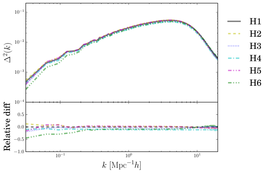
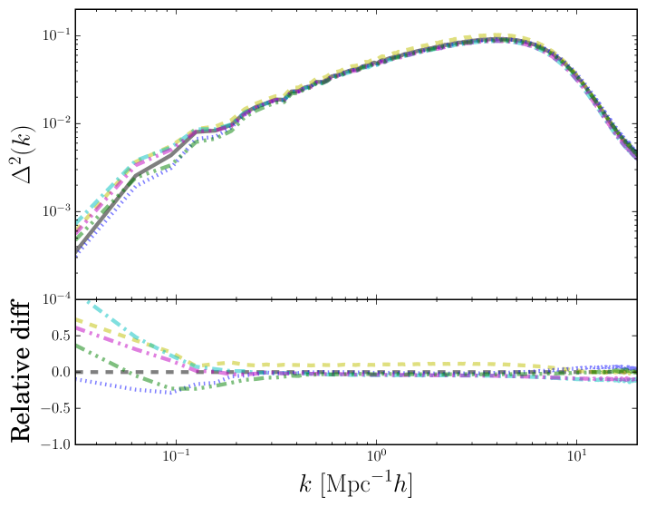
Figure 13 shows the three-dimensional power spectrum of the H i  Ly$\alpha$ forest flux. The general shape of the power spectrum is similar to that of the one-dimensional version seen in Figure 12, although the drop in power at high-$k$ is not as pronounced. More importantly, there are observable differences on large scales between the different reionization histories, which can differ by up to a factor of 2. Importantly, the gas power spectrum of all of the simulations is essentially identical on large scales, so all differences are due to the different ionization histories of the IGM and not to the the underlying matter or gas distribution.

The differences in power at large scales are likely due to the correlations in the radiation field in the IGM. As mentioned in McDonald (2003), differences in the thermal state of the IGM (either the temperature $T_{0}$ or the slope $\gamma$) only lead to differences at the $\sim 10\%$ level, which is consistent with the results seen in Figure 13. The differences on large scales are significantly larger than this and furthermore do not seem to be correlated with particular values of $T_{0}$ and $\gamma$. Indeed, when we compare this with the values in Figure 6, the power on large scales does not seem to be correlated with either value, further demonstrating that the thermal history alone is not responsible for the differences on large scales.

Proper characterization of the full three-dimensional power spectrum is important for measurements of the BAO from the Ly$\alpha$ forest (Busca et al., 2013; Slosar et al., 2013). As can be seen in Figure 13, there are differences on large scales, in some cases as large as a factor of two between the different reionization scenarios. Thus, properly understanding the impact that the reionization of helium has on the three-dimensional power spectrum is important for systematic errors for the BAO measurement.

6. Conclusion

In this paper, we have presented a new suite of simulations that couple $N$-body methods, hydrodynamics, and radiative transfer simultaneously in order to study helium ii reionization. Some of the most important observational implications that helium ii reionization leaves on the low-density gas of the IGM come from the dramatic increase in temperature from the photoheating of the gas. Using the results of the simulations, we summarize here several conclusions that we can make:

1. In addition to changing the ionization fraction of helium as a function of redshift $x_{\mathrm{HeIII}}(z)$, helium ii reionization also leaves an important signature on the thermal history of the IGM. This finding is consistent with previous studies of helium ii reionization, which suggest using the temperature of the IGM to learn about helium ii reionization. We show that the peak in the temperature at mean density as a function of redshift $T(z)$ is a relatively robust signifier of helium ii reionization, occurring when the volume is 90-95% ionized by volume. The redshift interval over which the temperature of the IGM increases can be used to determine the duration of reionization, although this measurement is observationally less straightforward.

2. Observations of synthetic H i  Ly$\alpha$ sightlines show that many statistics concerning the forest are similar when we control the value of $\tau_{\mathrm{eff}}$, although important differences caused by different thermal histories may still be detectable. In particular, the one-dimensional power spectrum and the flux PDF show important differences that can be understood in terms of the thermal state of the IGM. These differences can be substantial, especially in the small-scale one-dimensional power spectrum.

3. The three-dimensional flux power spectrum shows significant differences between the simulations, with differences on large scales of up to a factor of 2. Previous studies have attempted to measure this quantity (Slosar et al., 2011; Lee et al., 2014), although the error bars are still significant.

In future studies, we plan to investigate the effect that anisotropic sources have on helium ii reionization. The effect was discussed briefly in McQuinn et al. (2009), although we plan to explore this aspect more thoroughly. In addition, we plan to detect observational signatures in the Ly$\beta$ and Ly$\gamma$ forests. Iršič & Viel (2014) showed that temperature information of the IGM was better determined by studying the Ly$\beta$ forest and the cross-correlation with the Ly$\gamma$ forest. Additionally, these transitions saturate at much higher neutral hydrogen densities, and so they can give additional information about the thermal state of the IGM at higher densities. This type of comparison can provide an additional observational tool for understanding helium ii reionization, and provide another point of comparison with observations.

Appendix A Renormalizing $\tau_{\mathrm{eff}}$

In several previous observational studies of the H i  Ly$\alpha$ forest (Theuns et al., 2002; Bernardi et al., 2003; Dall’Aglio et al., 2008; Faucher-Giguère et al., 2008b), a dip in the effective optical depth $\tau_{\mathrm{eff}}$ at $z\sim 3.2$ was reported. It was proposed that this dip might be related to helium reionization. Several subsequent studies (Bolton et al., 2009a, b; McQuinn et al., 2009; Compostella et al., 2013) did not reproduce this feature. In particular, the functional form of $\tau_{\mathrm{eff}}(z)$ from Lee et al. (2015) does not include this feature. As explained in Section 2.3, the usual approach taken in the simulations is to renormalize the photoionization rate of galaxies $\Gamma_{\mathrm{gal}}$ in order to reproduce $\tau_{\mathrm{eff}}(z)$ by construction. As a result, the potential dip at $z\sim 3.2$ would not appear. To study whether this feature emerges from the simulations without renormalization, we have run Simulation H7, which uses the same simulation parameters as H1, but with $\Gamma_{\mathrm{gal}}$ provided by the model of HM12. To isolate the contribution of the galaxies, the authors of HM12 have furnished a series of photoionization rates and photoheating rates that only include the contribution from galaxies, and do not include quasars (P. Madau 2017, private communication). Thus, we are able to determine if the dip in $\tau_{\mathrm{eff}}$ can be reproduced in our simulations.

To explore the extent to which helium ii reionization affects the Ly$\alpha$ forest, we have not explicitly matched the value of $\tau_{\mathrm{eff}}$ for this simulation. The value of $\tau_{\mathrm{eff}}$ for Simulation H7 differs from that of the other simulations, although it does not differ by more than a factor of 2. Initially, the value of $\tau_{\mathrm{eff}}$ is greater than the other simulations (showing lower overall flux), and then crosses over to become lower than the other simulations around $z\sim 3$. Furthermore, there is no significant dip in $\tau_{\mathrm{eff}}$ at $z\sim 3.2$, or any other point in the evolution of the simulation. This lack of a feature in $\tau_{\mathrm{eff}}$ is consistent with more recent findings (Bolton et al., 2009a, b; McQuinn et al., 2009; Compostella et al., 2013).

Appendix B Renormalizing the Ly$\alpha$ Flux PDF

Figure 14.— Comparison of the Ly$\alpha$ forest flux PDF of Simulation H6 using the default value of $\tau_{\mathrm{eff}}$ from Lee et al. (2015) (labeled “fiducial” in the Figure) and a renormalized value of $\tau_{\mathrm{eff}}$ from Calura et al. (2012), as well as the data from Calura et al. (2012). The discrepancy at high flux values is smaller in the case of the renormalized value of $\tau_{\mathrm{eff}}$, which is consistent with the fact that the value of $\tau_{\mathrm{eff}}$ is lower for Calura et al. (2012). Nevertheless, the difference in the normalization cannot account for the whole discrepancy. As shown in Figure 8 of Calura et al. (2012), the continuum uncertainty can have a significant effect on the shape of the flux PDF. Thus, a proper estimation of the continuum level for observations is essential for understanding the flux PDF.

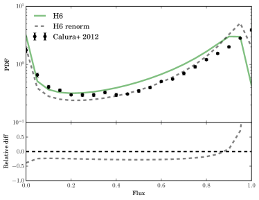
In Section 5.2 we discussed the results of measuring the Ly$\alpha$ forest flux PDF for the different simulations. In order to compare them against observation, Figure 10 shows the measurement of the flux PDF from Calura et al. (2012) at $z\sim 2.9$. There is a noticeable difference in the shape between the observational and simulated results. As explained in Section 5.2, there is a difference in the measured $\tau_{\mathrm{eff}}$ of the measurements compared to our simulations, which used the more recent measurements of Lee et al. (2015) to define the value of $\tau_{\mathrm{eff}}(z)$ that the simulations matched. In order to investigate whether the difference in the flux PDF shape could be attributed entirely to the different value of $\tau_{\mathrm{eff}}$, we adjusted the average flux absorption $\expectationvalue{F}$ of the volume to match the lower value of $\tau_{\mathrm{eff}}$ from Calura et al. (2012).

Figure 14 shows the flux PDF of Simulation H6 renormalized to have the same value of $\tau_{\mathrm{eff}}$ as Calura et al. (2012), and the measurements. The figure also shows the original flux PDF for the default normalization. The value of $\tau_{\mathrm{eff}}$ reported by Lee et al. (2015) is greater than the value reported by Calura et al. (2012). Accordingly, when the spectra have been renormalized to have the same value of $\tau_{\mathrm{eff}}$, some of the discrepancy between the simulations and the measurements has been removed. Nevertheless, there is still some difference between the measurements, especially for the bins of high flux ($F\sim 1$). Thus, this difference cannot be attributed entirely to the difference in $\tau_{\mathrm{eff}}$. As discussed in Calura et al. (2012), the placement of the continuum-level can have a significant effect on the shape of the flux PDF. Additionally, the difference in effective resolution between the simulations and the observations may also play some role.

Appendix C The Quasar Luminosity Function

Figure 15.— Evolution of the QLF parameters as a function of redshift: the base-ten logarithm of $\phi^{*}$ (top left), the break magnitude $M^{*}$ (top right), the faint-end slope $\alpha$ (bottom left), and the steep-end slope $\beta$ (bottom right). Best-fit values and associated 1$\sigma$ errors from R13, M12, and M13 are represented as the black circles, dark gray triangles, and light gray stars, respectively. The solid lines show the parameterization of the parameters given by Equations (C2a-C2d) based on these data, reproduced in Table 2. For the evolution of $\log_{10}\phi^{*}$, the dashed line shows the best-fit assuming only linear evolution in $z$ instead of quadratic, motivating an empirical need for quadratic evolution. See the text in Appendix C for further details.

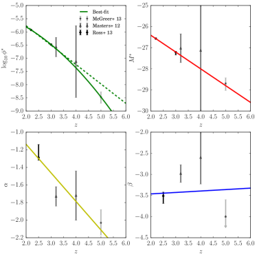
In Paper I, we provide a method for parameterizing the QLF as a function of redshift that combines measurements from Ross et al. (2013), Masters et al. (2012), and McGreer et al. (2013) (hereafter referred to as R13, M12, and M13). These observations provide fits for the QLF at redshifts $2.2\lesssim z\lesssim 3.5$, $z\sim 3.2$ and $z\sim 4$, and $z\sim 5$, respectively. All three works parameterize the QLF as a double-power law, defined by the same four parameters: $\phi^{*}$, the overall amplitude of the QLF with units of Mpc^-1 mag^-1; $\alpha$, the slope of the faint end of the QLF; $\beta$, the slope of the bright end; and $M^{*}$, the so-called break magnitude where the QLF transitions between the slopes $\alpha$ and $\beta$. Mathematically, the QLF can be written as

$$\phi(M)=\frac{\phi^{*}}{10^{0.4(\alpha+1)(M-M^{*})}+10^{0.4(\beta+1)(M-M^{*})}}.$$ (C1)

To combine the R13, M12, and M13 data sets into a single set of quantities, we cast the four parameters of the QLF ($\phi^{*}$, $M^{*}$, $\alpha$, and $\beta$) as quantities that have evolution in redshift. We define these parameters as

$$\log_{10}\phi^{*}(z) =\log_{10}\phi^{*}_{0}+c_{1}(z-3)+c_{2}(z-3)^{2},$$ (C2a)

$$M^{*}(z) =M^{*}_{0}+c_{3}(z-3),$$ (C2b)

$$\alpha(z) =\alpha_{0}+c_{4}(z-3),$$ (C2c)

$$\beta(z) =\beta_{0}+c_{5}(z-3).$$ (C2d)

For the case of the overall normalization $\log_{10}\phi^{*}$, we include quadratic evolution with redshift. The comoving number density of quasars is not monotonic and peaks at $z\sim 2$ (e.g., Figure 20 of Richards et al. 2006). Accordingly, there is a significant decrease in the overall amplitude in the QLF at high redshifts, and the redshift evolution is not well fit by a single linear term. Thus, observations suggest that the redshift evolution of this parameter is not purely linear over such a large span in redshift. (See Figure 15 for a comparison between a linear and quadratic fit.) The other parameters have redshift evolutions that are fit adequately with simple linear evolution in redshift, and so we only include linear terms to avoid overfitting.

Table 2Best-fit Parameters in Equations (C2a-C2d) Given the Data Listed in R13, M12, and M13.

Parameter	Best-fit Value
$\log_{10}\phi^{*}_{0}$	$-6.48$
$c_{1}$	$-0.776$
$c_{2}$	$-0.109$
$M^{*}_{0}$	$-27.2$
$c_{3}$	$-0.795$
$\alpha_{0}$	$-1.46$
$c_{4}$	$-0.324$
$\beta_{0}$	$-3.43$
$c_{5}$	$\phantom{-}0.0342$

Note. — These parameters provide a fit to the luminosity function through redshift and ensure that the abundance of quasars matches observations as best possible. For additional details on the parameters and the fitting procedure, see the text in Appendix C.

We now briefly summarize the relevant findings of R13, M12, and M13. In all three results, the QLF is parameterized as a double-power law, according to Equation (C1). R13 uses quasars identified from SDSS-III Data Release 9 (DR9), and provides a luminosity-evolution density-evolution (LEDE) model in which the base-10 logarithm of the QLF normalization, $\log_{10}\phi^{*}$, and the break magnitude $M^{*}$, evolve linearly with redshift. The parameters $\alpha$ and $\beta$ are fixed as a function of redshift. Nominally, the LEDE fit is valid over the redshift range $2.2\leq z\leq 3.5$. M12 uses data from the COSMOS survey, and measures the four QLF parameters at $z\sim 3.2$ and $z\sim 4$. M13 uses quasars identified in SDSS data in Stripe 82 (S82), and reports the four QLF parameters at $z\sim 5$. For all three results, the parameters themselves and their associated 1$\sigma$ uncertainties are reported. The one exception to this is the value of $\beta$ from the M13 measurements, which was fixed to a value of $\beta=-4$. The authors report that the value was fixed during the fits since allowing the bright-end slope to take on any value would result in arbitrarily steep value of $\beta$. The authors of M13 state that this is due to the low number count of objects at very bright magnitudes. In order to prevent against the value from being fixed in our composite QLF, we parameterize $\beta$ as being an upper limit, with 1$\sigma$ scatter above the value of $\beta=-4$ of $\sigma=0.4$. This value is inferred from Figure 18 of M13, which shows the joint likelihood of $\beta$ and $M^{*}$, the break magnitude. At 68% confidence, the authors report $\beta<-3.6$.

It should also be pointed out that M12 and M13 use different magnitude conventions from the data in R13. Rather than reporting $M_{i}(z=2)$, the absolute $i$-band magnitude at $z=2$, M12 and M13 report magnitudes as $M_{1450}$, the absolute magnitude at 1450 Å. In order to convert between these two systems, we follow the convention of R13 and use $M_{i}(z=2)=M_{1450}-1.486$ (Ross et al., 2013, Appendix B). We should mention, however, that this conversion assumes a power-law slope of $\alpha=0.5$ ($f_{\nu}\propto\nu^{-\alpha}$) and changes slightly for different spectral indices. Ultimately, the conversion between different magnitude systems is not important for our overall conclusions because for most of our simulation models, the observables we are most interested in (especially the peak in the IGM temperature, Figure 7) are dominated by the QLF at redshifts $z\leq 3.5$. At these redshifts, the QLF is determined with very small statistical uncertainty by the measurements of R13, and thus no conversion between magnitude systems is necessary.

C.1. Model Q1

To combine the data from the different data sets, we fit for the four QLF parameters independently as a function of redshift. The parameters are assumed to vary linearly in redshift, except for the base-10 logarithm of the normalization, which includes quadratic evolution. As explained above, we would expect that a purely linear fit of this quantity is not adequate over such a large range in redshift, since the total quasar number density peaks around $z\sim 2$ and turns over. The equations for the parameters are given in Equations (C2a-C2d), and the resulting best-fit values for the parameters and uncertainties given in Table 2. Instead of fitting for the evolution of the four parameters independently, it would be better to find a simultaneous fit to all of the data spanning the entire redshift range. However, many degeneracies exist between these parameters, and finding a simultaneous fit to adequately describe all of the data over a very large redshift range is difficult to achieve.

Figure 15 shows the measured parameters as a function of redshift, as well as the best-fit line for each parameter. As explained above, for the QLF normalization $\log_{10}\phi^{*}$ and break magnitude $M^{*}$, we include the parameters from R13 at $z=2.2$, where the parameters are determined best, and at $z=3$, in order to provide good constraints on the overall normalization at a slightly higher redshift. Combined with the two points from M12 ($z=3.2$ and $z=4$) and the single point from M13 ($z=5$), there are five total data points that are fit. We include $\alpha$ and $\beta$ from R13 at $z=2.5$, since there is no explicit redshift dependence included in the R13 fits. Nevertheless, the reported parameters from higher redshift data (and even when we compare the binned data from $z\sim 3$ in the R13 data) apparently show no redshift evolution particularly for $\alpha$. Therefore, our model includes redshift evolution in these parameters. At $z\sim 2.5$, there is very good agreement between the binned QLF and the fit model of R13. However, the fit values are ultimately not very sensitive to the choice of redshift. Combined with the results from M12 and M13, this creates four data points to fit. The fit for all of the parameters is reasonably good, with the notable exception of the steep-end slope $\beta$. As mentioned earlier, constraining $\beta$ is observationally difficult because of the low number count of objects. It is also worth noting that the fits of M12 do not directly constrain $\beta$ with their data. Their measurements from the COSMOS field are primarily for faint objects and are fainter than the break magnitude $M^{*}$. In order to determine $\beta$ in their fits, M12 use measurements from Richards et al. (2006) to provide observations of bright objects. The overall result is little evolution in $\beta$ over the redshift interval $2.5\lesssim z\lesssim 5$, with perhaps a slight steepening at lower redshifts. This trend is opposite to the trend of $\alpha$, which shows a very clear trend of becoming shallower at lower redshifts. Nevertheless, owing to the low overall amplitude of the luminosity function at high magnitudes, the precise value of $\beta$ does not significantly affect the predictions for reionization.

C.2. Model Q2

An alternative to finding the best-fit parameterizations is to simply interpolate between the values reported in R13, M12, and M13. To this end, we assume that the values for the parameters $\phi^{*}$, $M^{*}$, $\alpha$, and $\beta$ reported by the different studies are accurate for their respective redshift ranges. Specifically, we use the values reported by R13 for redshifts $z\leq 3.5$, the values of M12 at $z\sim 4$, and the values of M13 for redshifts of $z\geq 5$. In order to determine values of the parameters at intermediate redshifts, we linearly interpolate in redshift. This method produces a QLF that is consistent with the different measurements by construction, but can introduce some features into the QLF evolution through the naïve linear interpolation method. We therefore regard Model Q1 as our fiducial model and present this alternative merely as a point of comparison.

Appendix D Galaxy Photoionization Rates

When presenting the methods of the simulations in Section 2.3, we note that this work introduces the concept of renormalizing the photoionization rate of galaxies $\Gamma_{\mathrm{gal}}$ on-the-fly by computing the Ly$\alpha$ forest effective optical depth of the volume to match observational constraints. In this appendix, we directly compare directly the photoionization rates of the different simulations.

As explained in Section 2.3, the value of $\Gamma_{\mathrm{gal}}$ is increased or decreased to agree by construction with the value of $\tau_{\mathrm{HI}}$ as determined by Lee et al. (2015). However, if the value of $\Gamma_{\mathrm{gal}}$ were to decrease below a value of $\Gamma_{\mathrm{gal}}=10^{-13}$ s^-1, then the photon output of quasars is decreased instead. This decrease prevents $\Gamma_{\mathrm{gal}}$ from dropping below levels that are far below the levels determined theoretically (Haardt & Madau, 2012) or observationally (Faucher-Giguère et al., 2008a).

Figure 16.— From top to bottom: the combined galaxy photoionization rate $\Gamma_{\mathrm{gal}}$, quasar photoionization rate $\Gamma_{\mathrm{qso}}$, total photoionization rate $\Gamma_{\mathrm{tot}}$, and quasar photon production rate $x_{\mathrm{qso}}$ as a function of redshift for each of the simulations presented in this work. In the top plot we also plot the value of $\Gamma_{\mathrm{gal}}$ from Haardt & Madau (2012). Simulation H6 does not have explicit quasar sources and so does not have values for $\Gamma_{\mathrm{qso}}$ or $x_{\mathrm{qso}}$.

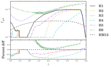
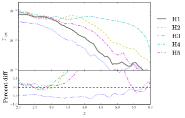
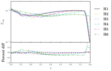
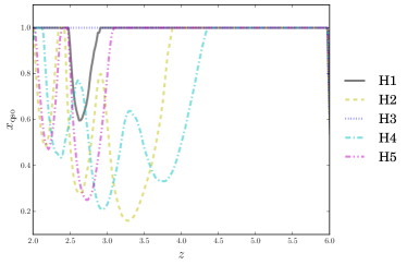
Figure 16 shows four different quantities as a function of redshift: the photoionization rate from galaxies $\Gamma_{\mathrm{gal}}$, the photoionization rate from quasars $\Gamma_{\mathrm{qso}}$, the total photoionization rate $\Gamma_{\mathrm{tot}}=\Gamma_{\mathrm{gal}}+\Gamma_{\mathrm{qso}}$, and the multiplicative factor for quasar photon production $x_{\mathrm{qso}}$. This last factor is applied to each quasar source at each time step in the simulation as

$$N_{\gamma,\mathrm{actual}}=x_{\mathrm{qso}}N_{\gamma,\mathrm{catalog}}.$$ (D1)

A value of $x_{\mathrm{qso}}=1$ represents quasars producing as many photons as dictated by the naïve calculation of the catalog, with the value $x_{\mathrm{qso}}<1$ to ensure that $\Gamma_{\mathrm{gal}}\geq 10^{-13}$ s^-1, while still being able to match the overall Ly$\alpha$ forest optical depth (see Figure 9).

The top panel of Figure 16 shows the value of $\Gamma_{\mathrm{gal}}$ for all of the simulations, as well as for the semi-analytic calculation of Haardt & Madau (2012). A minimum value of $\Gamma_{\mathrm{gal}}=10^{-13}$ s^-1 is imposed, which corresponds to values of $x_{\mathrm{qso}}<1$ in the bottom panel. Moreover, most of the simulations have comparable values of $\Gamma_{\mathrm{tot}}$, to within about 10%. This makes sense, since the value of $\Gamma_{\mathrm{tot}}$ is closely related to $\tau_{\mathrm{eff,HI}}$, which is matched between the simulations by construction.

Appendix E Number of Frequency Bins

Table 3Frequency Bins Used in the Radiative Transfer Calculations.

Frequency Bin	Left Edge	Right Edge	Central Value

1 & 13.6 24.6 17.6
2 24.6 54.4 34.2
3 54.4 65 59.3
4 65 75 69.7
5 75 125 94.2
6 125 250 168
7 250 1000 410

Note. — This choice for the distribution of frequency bins shows agreement with $N=50$ frequency bins to about 2% in observed temperature in a test simulation. This translates into a precision of about 400 K.

An important parameter for radiative transfer calculations is the number of frequency bins used in the calculation. This creates a trade-off in accuracy of certain quantities in the simulation, most notably the temperature as a result of photoheating, and computational resources required for computation. Increasing the number of frequency bins requires additional memory and computation time, which tend to scale linearly with the number of frequency bins. Thus, finding the fewest number of bins for a given accuracy is of great importance.

Figure 17.— The temperature in spherically averaged shells at a distance of $r$ (in grid units) from a single quasar source versus the computed temperature (in K) for different choices of the number of frequency bins. Top: a uniform medium of density $\Delta=10$; bottom: density $\Delta=1$. The different colors show different times of the simulation, and different line styles show the number of frequency bins used to compute helium reionization ($54.4~{}\mathrm{eV}\leq h\nu\leq 1~{}\mathrm{keV}$). The relative difference in the lower panel shows that the scheme chosen in the main body of the text, listed explicitly in Table 3, exhibits significantly better convergence than selecting bins which are more regularly spaced. The differences shown here correspond to absolute temperature differences of about 400 K for $\Delta\sim 10$, and less than 100 K for $\Delta\sim 1$.

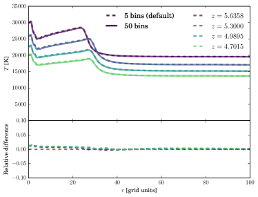
In the simulations presented here, we have used a total of seven frequency bins to accurately capture the thermal state of the IGM: one bin between the 13.6 and 24.6 eV (photons only energetic enough to ionize H i), one bin between 24.6 and 54.6 eV (which ionize both H i and He i), and five frequency bins between 54.4 eV and 1 keV (which are capable of ionizing H i, He i, and He ii). The distribution of the bins is not regularly spaced but instead more finely samples the frequencies closer to the He ii edge (as a result of the steeply dropping cross-section of He ii with frequency).

A further consideration is which choice to make for the “center” of the frequency bin, since this affects the actual amount of heat deposited in the gas when we compute photoheating rates. For the bin centers, we choose the energy-weighted photon number produced by quasars, which depends only on the spectral index $\alpha$ and not the overall normalization. If the luminosity of a quasar as a function of frequency is written as $L(\nu)=L_{0}\nu^{-\alpha}$, then the number of photons produced is $N_{\gamma}=\int L_{0}\nu^{-\alpha}/(h\nu)\differential{\nu}$. The energy-weighted number of photons from quasars is therefore

$$\expectationvalue{N_{\gamma}}_{E}=\frac{\int h\nu\frac{L_{0}\nu^{-\alpha}}{h\nu}\differential{\nu}}{\int\frac{L_{0}\nu^{-\alpha}}{h\nu}\differential{\nu}}.$$ (E1)

By choosing this convention, the bin centers are optimal for calculating the photoheating of gas. Table 3 summarizes the properties of the photon bins used in the body of the paper.

In order to test for the numerical convergence of temperature given the number of bins we used, we ran a series of test simulations while increasing the number of frequency bins we used. These simulations featured a single source placed at the center of a uniform cubic volume. We compare the five bin edges used in this simulation with five bins whose edges are distributed on logarithmically even intervals. We also use a simulation with 25 logarithmically spaced intervals and 50 logarithmically spaced ones. These simulations with 50 frequency bins are treated as the “ground truth” simulations for the purposes of comparison. This approach is similar to the approaches discussed in the appendices of McQuinn et al. (2009) and Compostella et al. (2013).

Figure 17 shows the spherically averaged temperature as a function of radius for the different number of frequency bins we used. The different line colors show the simulations at different times (given as redshifts), and different line styles represent different numbers of frequency bins. The top panel shows the difference in temperature in a uniform medium of constant density $\Delta=10$ and the lower panel shows the same for $\Delta=1$. The lower axis in each panel shows the relative difference compared to the $N=50$ simulation. In general, the number and distribution of the frequency bins used in the simulation show fairly good agreement with the $N=50$ simulations. In particular, a more naïve choice of $N=5$ logarithmically spaced bins shows poor numerical convergence, differing from the $N=50$ case by as much as 10% at some places. The choice of bins used in the body of the work deviates by at most about 2%, a much more modest amount. In terms of absolute temperature, this corresponds to a difference of about 400 K. The relative difference is much smaller in low-density regions, and so we expect the temperature calculation to remain accurate for the majority of regions probed by the Ly$\alpha$ statistics discussed in the body of the paper. In summary, by choosing bins that oversample the frequency bins near the He ii edge, much better temperature convergence can be achieved than by selecting a distribution that is more equitably sampled. At the same time, the shape of the SED of quasars also has a significant effect on the inferred temperature induced by photoheating and represents a much larger systematic error than the number of frequency bins used in the radiative transfer scheme.

References

- Battaglia et al. (2013) Battaglia, N., Trac, H., Cen, R., & Loeb, A. 2013, ApJ, 776, 81
- Becker & Bolton (2013) Becker, G. D., & Bolton, J. S. 2013, MNRAS, 436, 1023
- Becker et al. (2011a) Becker, G. D., Bolton, J. S., Haehnelt, M. G., & Sargent, W. L. W. 2011a, MNRAS, 410, 1096
- Becker et al. (2013) Becker, G. D., Hewett, P. C., Worseck, G., & Prochaska, J. X. 2013, MNRAS, 430, 2067
- Becker et al. (2007) Becker, G. D., Rauch, M., & Sargent, W. L. W. 2007, ApJ, 662, 72
- Becker et al. (2011b) Becker, G. D., Sargent, W. L. W., Rauch, M., & Calverley, A. P. 2011b, ApJ, 735, 93
- Bernardi et al. (2003) Bernardi, M., Sheth, R. K., SubbaRao, M., et al. 2003, AJ, 125, 32
- Bolton & Haehnelt (2007) Bolton, J. S., & Haehnelt, M. G. 2007, MNRAS, 382, 325
- Bolton et al. (2009a) Bolton, J. S., Oh, S. P., & Furlanetto, S. R. 2009a, MNRAS, 395, 736
- Bolton et al. (2009b) —. 2009b, MNRAS, 396, 2405
- Bolton et al. (2016) Bolton, J. S., Puchwein, E., Sijacki, D., et al. 2016, ArXiv e-prints, arXiv:1605.03462
- Busca et al. (2013) Busca, N. G., Delubac, T., Rich, J., et al. 2013, A&A, 552, A96
- Calura et al. (2012) Calura, F., Tescari, E., D’Odorico, V., et al. 2012, MNRAS, 422, 3019
- Calverley et al. (2011) Calverley, A. P., Becker, G. D., Haehnelt, M. G., & Bolton, J. S. 2011, MNRAS, 412, 2543
- Caucci et al. (2008) Caucci, S., Colombi, S., Pichon, C., et al. 2008, MNRAS, 386, 211
- Cen & Safarzadeh (2015a) Cen, R., & Safarzadeh, M. 2015a, ApJ, 798, L38
- Cen & Safarzadeh (2015b) —. 2015b, ApJ, 809, L32
- Cen & Safarzadeh (2016) —. 2016, ArXiv e-prints, arXiv:1604.06473
- Ciardi et al. (2003) Ciardi, B., Ferrara, A., & White, S. D. M. 2003, MNRAS, 344, L7
- Cisewski et al. (2014) Cisewski, J., Croft, R. A. C., Freeman, P. E., et al. 2014, MNRAS, 440, 2599
- Compostella et al. (2013) Compostella, M., Cantalupo, S., & Porciani, C. 2013, MNRAS, 435, 3169
- Compostella et al. (2014) —. 2014, MNRAS, 445, 4186
- Croft et al. (1998) Croft, R. A. C., Weinberg, D. H., Katz, N., & Hernquist, L. 1998, ApJ, 495, 44
- Dall’Aglio et al. (2008) Dall’Aglio, A., Wisotzki, L., & Worseck, G. 2008, A&A, 491, 465
- D’Aloisio et al. (2016) D’Aloisio, A., Upton Sanderbeck, P. R., McQuinn, M., Trac, H., & Shapiro, P. R. 2016, ArXiv e-prints, arXiv:1607.06467
- Dawson et al. (2013) Dawson, K. S., Schlegel, D. J., Ahn, C. P., et al. 2013, AJ, 145, 10
- Dijkstra et al. (2004) Dijkstra, M., Lidz, A., & Hui, L. 2004, ApJ, 605, 7
- Dixon & Furlanetto (2009) Dixon, K. L., & Furlanetto, S. R. 2009, ApJ, 706, 970
- Faucher-Giguère et al. (2008a) Faucher-Giguère, C.-A., Lidz, A., Hernquist, L., & Zaldarriaga, M. 2008a, ApJ, 682, L9
- Faucher-Giguère et al. (2008b) Faucher-Giguère, C.-A., Prochaska, J. X., Lidz, A., Hernquist, L., & Zaldarriaga, M. 2008b, ApJ, 681, 831
- Furlanetto & Oh (2008) Furlanetto, S. R., & Oh, S. P. 2008, ApJ, 681, 1
- Furlanetto & Stoever (2010) Furlanetto, S. R., & Stoever, S. J. 2010, MNRAS, 404, 1869
- Gnedin & Hui (1998) Gnedin, N. Y., & Hui, L. 1998, MNRAS, 296, 44
- Gunn & Peterson (1965) Gunn, J. E., & Peterson, B. A. 1965, ApJ, 142, 1633
- Haardt & Madau (1996) Haardt, F., & Madau, P. 1996, ApJ, 461, 20
- Haardt & Madau (2012) —. 2012, ApJ, 746, 125
- Hinshaw et al. (2013) Hinshaw, G., Larson, D., Komatsu, E., et al. 2013, ApJS, 208, 19
- Hjerting (1938) Hjerting, F. 1938, ApJ, 88, 508
- Hopkins et al. (2007) Hopkins, P. F., Richards, G. T., & Hernquist, L. 2007, ApJ, 654, 731
- Hui & Gnedin (1997) Hui, L., & Gnedin, N. Y. 1997, MNRAS, 292, 27
- Iršič & Viel (2014) Iršič, V., & Viel, M. 2014, J. Cosmology Astropart. Phys, 12, 024
- Jakobsen et al. (1994) Jakobsen, P., Boksenberg, A., Deharveng, J. M., et al. 1994, Nature, 370, 35
- Jena et al. (2005) Jena, T., Norman, M. L., Tytler, D., et al. 2005, MNRAS, 361, 70
- Kimm & Cen (2014) Kimm, T., & Cen, R. 2014, ApJ, 788, 121
- La Plante & Trac (2015) La Plante, P., & Trac, H. 2015, ArXiv e-prints, arXiv:1507.03021
- Lee et al. (2013) Lee, K.-G., Bailey, S., Bartsch, L. E., et al. 2013, AJ, 145, 69
- Lee et al. (2014) Lee, K.-G., Hennawi, J. F., Stark, C., et al. 2014, ApJ, 795, L12
- Lee et al. (2015) Lee, K.-G., Hennawi, J. F., Spergel, D. N., et al. 2015, ApJ, 799, 196
- Lewis et al. (2000) Lewis, A., Challinor, A., & Lasenby, A. 2000, ApJ, 538, 473
- Lu et al. (1996) Lu, L., Sargent, W. L. W., Womble, D. S., & Takada-Hidai, M. 1996, ApJ, 472, 509
- Lukić et al. (2015) Lukić, Z., Stark, C. W., Nugent, P., et al. 2015, MNRAS, 446, 3697
- Lusso et al. (2015) Lusso, E., Worseck, G., Hennawi, J. F., et al. 2015, MNRAS, 449, 4204
- Masters et al. (2012) Masters, D., Capak, P., Salvato, M., et al. 2012, ApJ, 755, 169
- McDonald (2003) McDonald, P. 2003, ApJ, 585, 34
- McDonald & Eisenstein (2007) McDonald, P., & Eisenstein, D. J. 2007, Phys. Rev. D, 76, 063009
- McDonald et al. (2005) McDonald, P., Seljak, U., Cen, R., Bode, P., & Ostriker, J. P. 2005, MNRAS, 360, 1471
- McDonald et al. (2006) McDonald, P., Seljak, U., Burles, S., et al. 2006, ApJS, 163, 80
- McGreer et al. (2013) McGreer, I. D., Jiang, L., Fan, X., et al. 2013, ApJ, 768, 105
- McQuinn et al. (2011) McQuinn, M., Hernquist, L., Lidz, A., & Zaldarriaga, M. 2011, MNRAS, 415, 977
- McQuinn et al. (2009) McQuinn, M., Lidz, A., Zaldarriaga, M., et al. 2009, ApJ, 694, 842
- Meiksin & Tittley (2012) Meiksin, A., & Tittley, E. R. 2012, MNRAS, 423, 7
- Meiksin et al. (2010) Meiksin, A., Tittley, E. R., & Brown, C. K. 2010, MNRAS, 401, 77
- Møller & Jakobsen (1990) Møller, P., & Jakobsen, P. 1990, A&A, 228, 299
- Myers et al. (2015) Myers, A. D., Palanque-Delabrouille, N., Prakash, A., et al. 2015, ApJS, 221, 27
- Ozbek et al. (2016) Ozbek, M., Croft, R. A. C., & Khandai, N. 2016, MNRAS, 456, 3610
- Palanque-Delabrouille et al. (2013) Palanque-Delabrouille, N., Yèche, C., Borde, A., et al. 2013, A&A, 559, A85
- Palanque-Delabrouille et al. (2015) Palanque-Delabrouille, N., Yeche, C., Baur, J., et al. 2015, ArXiv e-prints, arXiv:1506.05976
- Pichon et al. (2001) Pichon, C., Vergely, J. L., Rollinde, E., Colombi, S., & Petitjean, P. 2001, MNRAS, 326, 597
- Puchwein et al. (2015) Puchwein, E., Bolton, J. S., Haehnelt, M. G., et al. 2015, Monthly Notices of the Royal Astronomical Society, 450, 4081
- Reimers et al. (1997) Reimers, D., Kohler, S., Wisotzki, L., et al. 1997, A&A, 327, 890
- Richards et al. (2006) Richards, G. T., Strauss, M. A., Fan, X., et al. 2006, AJ, 131, 2766
- Ross et al. (2013) Ross, N. P., McGreer, I. D., White, M., et al. 2013, ApJ, 773, 14
- Shang et al. (2011) Shang, Z., Brotherton, M. S., Wills, B. J., et al. 2011, ApJS, 196, 2
- Shull (1979) Shull, J. M. 1979, ApJ, 234, 761
- Slosar et al. (2011) Slosar, A., Font-Ribera, A., Pieri, M. M., et al. 2011, J. Cosmology Astropart. Phys, 9, 001
- Slosar et al. (2013) Slosar, A., Iršič, V., Kirkby, D., et al. 2013, J. Cosmology Astropart. Phys, 4, 26
- Syphers et al. (2009a) Syphers, D., Anderson, S. F., Zheng, W., et al. 2009a, ApJS, 185, 20
- Syphers et al. (2012) —. 2012, AJ, 143, 100
- Syphers & Shull (2014) Syphers, D., & Shull, J. M. 2014, ApJ, 784, 42
- Syphers et al. (2009b) Syphers, D., Anderson, S. F., Zheng, W., et al. 2009b, ApJ, 690, 1181
- Tepper-García (2006) Tepper-García, T. 2006, MNRAS, 369, 2025
- Theuns et al. (2002) Theuns, T., Bernardi, M., Frieman, J., et al. 2002, ApJ, 574, L111
- Theuns et al. (1998) Theuns, T., Leonard, A., Efstathiou, G., Pearce, F. R., & Thomas, P. A. 1998, MNRAS, 301, 478
- Trac & Cen (2007) Trac, H., & Cen, R. 2007, ApJ, 671, 1
- Trac et al. (2008) Trac, H., Cen, R., & Loeb, A. 2008, ApJ, 689, L81
- Trac et al. (2015) Trac, H., Cen, R., & Mansfield, P. 2015, ApJ, 813, 54
- Upton Sanderbeck et al. (2016) Upton Sanderbeck, P. R., D’Aloisio, A., & McQuinn, M. J. 2016, MNRAS, 460, 1885
- Viel et al. (2013) Viel, M., Becker, G. D., Bolton, J. S., & Haehnelt, M. G. 2013, Phys. Rev. D, 88, 043502
- White et al. (2012) White, M., Myers, A. D., Ross, N. P., et al. 2012, MNRAS, 424, 933
- Worseck et al. (2014) Worseck, G., Prochaska, J. X., Hennawi, J. F., & McQuinn, M. 2014, ArXiv e-prints, arXiv:1405.7405
- Worseck et al. (2011) Worseck, G., Prochaska, J. X., McQuinn, M., et al. 2011, ApJ, 733, L24
- Zheng et al. (2005) Zheng, W., Anderson, S. F., Kriss, G. A., et al. 2005, in IAU Colloq. 199: Probing Galaxies through Quasar Absorption Lines, ed. P. Williams, C.-G. Shu, & B. Menard, 484–486
- Zheng et al. (2008) Zheng, W., Meiksin, A., Pifko, K., et al. 2008, ApJ, 686, 195