Tethered membranes do not remain flat for strong structural asymmetry

Abstract

We set up the statistical mechanics for a nearly flat, thermally equilibrated fluid membrane, attached to an elastic network through one of its sides. We predict that the resulting structural (inversion) asymmetry of the membrane, notably due to the elastic network attached to one of its sides, can generate a local spontaneous curvature $C_{0}$, that may in turn destabilize the otherwise flat membrane. As $C_{0}$ rises above a threshold at a fixed temperature, a flat tethered membrane in the thermodynamic limit becomes structurally unstable, signaling crumpling of the flat membrane. In-vitro experiments on red blood cell membranes after depletion of adenosine-tri-phosphate molecules and artificial deposition of spectrin filaments on lipid bilayers may be used to verify our results.

Statistical flatness, a well-known feature of inversion-symmetric tethered or polymerized membranes at sufficiently low temperature ($T$) is marked by orientational long range order (LRO) weinberg . Examples of tethered membranes are plentiful covering biological Pontes ; Giess ; munro , physical wiese ; md-tethered ; mcs ; moldovan to chemical sinner systems. Red blood cell (RBC) membranes are one of the most well-known biological realizations of polymerized membranes joanny1 ; joanny2 . Statistical properties of inversion-symmetric tethered membranes have been extensively studied by now, see, e.g., Refs. weinberg ; chaikin . For instance, these membranes show a low-$T$ statistically flat phase weinberg ; chaikin , and a second order crumpling transition to a high-$T$ crumpled phase weinberg ; peliti2 . Furthermore, the scaling exponents that characterize the small fluctuations in the low-$T$ flat phase have been calculated within perturbative renormalization group (RG) framework. These are however idealizations of more general inversion-asymmetric tethered membranes. For instance, both in-vivo RBC membranes and in-vitro spectrin-deposited model lipid bilayers are structurally or inversion asymmetric, owing to the attachment of the elastic network on one side of the membrane. These have no theory to date. Understanding how structural asymmetry affects the statistical properties of nearly flat tethered membranes forms the principal motivation of this study.

Here we construct a coarse-grained continuum model for a fluid membrane attached to an elastic network on one side, in thermal equilibrium; see Fig. 1 for schematic model diagrams. We use it to investigate the effects of asymmetry on membrane conformation fluctuations. We uncover a novel structural instability in the flat membrane at fixed $T$, controlled by the local strain-dependent spontaneous curvature $C_{0}$, a direct measure of the degree of asymmetry. This indicates a novel asymmetry-induced crumpling of the membrane weinberg ; luca . Our results are generic in nature and can be tested in adenosine-tri-phosphate (ATP) depleted RBC membranes in equilibrium or in-vitro deposition of spectrin filaments on a model lipid bilayer artificial . In addition, our theory should be a starting point to construct a generic hydrodynamic description for live RBC membranes joanny1 ; joanny2 .

In order to construct a minimal coarse-grained model designed to extract the essential physics of the problem, we consider a tensionless fluid membrane with a bending modulus $\kappa_{0}$ in thermal equilibrium. The fixed connectivity spectrin network, attached to one side of the membrane, is treated as an elastic continuum parametrized by the appropriate Lamé constants or elastic modulii $\mu,\lambda>0$ weinberg ; chaikin in the long wavelength limit (valid over length scales $\gg$ typical spectrin mesh size $\sim 50nm$ safran ) . In stark contrast to their symmetric counterparts, we show that nearly flat asymmetric tethered membranes in equilibrium becomes structurally unstable yielding a crumpled state, controlled by $C_{0}$. From our theory, we show that the membrane (i) always remains statistically flat with LRO in thermodynamic limit (TL) for low $C_{0}$, (ii) stays flat for system size $L$ smaller than a persistence length $\xi$ (see below) and becomes unstable for $L>\xi$, for an intermediate range of $C_{0}$, implying a diverging $\langle C_{0}\rangle$ for $L>\xi$, and (iii) gets unstable for any $L$, large or small, for large enough $C_{0}$.

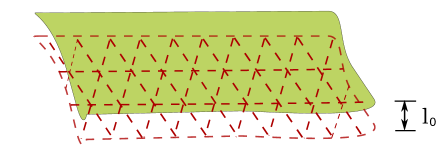
Figure 1: (color online) Schematic top view of a membrane (black quadrangle) coupled to an elastic network (broken red triangular lattice) on the bottom side, $l_{0}$ is the average distance between the two. The membrane and the elastic network are joined at the lattice points (see, e.g., Ref. alberts for RBC membrane structures, not shown in this diagram); see text.

We consider the spectrin layer - lipid membrane interaction in a strong coupling limit, i.e., strong interactions without any dissociation between them joanny . General symmetry considerations (i.e., invariance under translation and rotation) then dictate the form of the free energy functional $\mathcal{F}$ for a nearly flat asymmetric tethered membrane. In the coarse-grained long wavelength limit, we describe the membrane conformations by a single-valued field $h({\bf r})$ in the Monge gauge and lateral displacement by a two-dimensional ($2d$) vector field ${\bf u}({\bf r})$ weinberg ; chaikin . For simplicity we assume a fixed distance $l_{0}$ between the lipid membrane and the spectrin network; we ignore self-avoidance, and any relative motion between the spectrin network and the lipid membrane. We also ignore any defect, e.g., missing bonds in the spectrin network. Then, ${\mathcal{F}}$ takes the form

$${\mathcal{F}} = \frac{1}{2}\int d^{2}r[\kappa_{0}(\nabla^{2}h)^{2}+\lambda u_{ii}^{2}$$ (1)

$$+ 2\mu u_{ij}u_{ij}+2\chi u_{ii}\nabla^{2}h],$$

to the leading order in gradients; $r=|{\bf r}|$, ${\bf r}=(x,y)$ with (${\bf r},h$) denoting the coordinate of a point on the membrane in the three-dimensional embedding space. Here strain tensor $u_{ij}=\frac{1}{2}(\nabla_{i}u_{j}+\nabla_{j}u_{i}+\nabla_{i}h\nabla_{j}h)$, ignoring terms quadratic in $\nabla_{i}u_{j}$, which are irrelevant here in a scaling sense chaikin . In (1) we have included a generic inversion-symmetry breaking term $\chi\nabla^{2}hu_{ii}$, that couples local compressibility of the network with the local mean curvature. In the symmetric limit $\chi=0$; see Ref. safran for a model of RBC in terms of a solid and fluid membrane without the $\chi$-term. Free energy $\mathcal{F}$ implies a local spontaneous curvature $C_{0}=(\chi/\kappa_{0})u_{ii}$, which scales with $\chi$ and naturally vanishes in the symmetric limit. A larger $\chi^{2}$ signifies that a local spectrin compressibility induces a larger local mean curvature. Parameter $\chi$ can be positive or negative; a reversal in the sign of $\chi$ merely reverses $C_{0}$. We show below that $\chi^{2}$, or equivalently, the magnitude of $C_{0}$ controls the crumpling of an otherwise flat membrane.

We resolve $\bf u$ as $u_{i}=u_{i}^{L}+u_{i}^{T}$, where $u_{i}^{L}=q_{i}q_{j}u_{j}/q^{2}$ and $u_{i}^{T}=P_{ij}u_{j}$ are longitudinal and transverse components of $u_{i}$, respectively, for wavevector $\bf q$; $P_{ij}({\bf q})=\delta_{ij}-q_{i}q_{j}/q^{2}$ is the transverse projection operator operator , $i,j=x,y$. Thus up to the bilinear order in fields, free energy (1) takes the form

$${\mathcal{F}}_{g} = \int\frac{d^{2}q}{(2\pi)^{2}}[\frac{\kappa_{0}}{2}q^{4}|h({\bf q})|^{2}+(\frac{\lambda}{2}+\mu)\{q^{2}|u^{L}({\bf q})|^{2}$$ (2)

$$- \frac{2iq\chi h({\bf q})u^{L}({\bf-q})}{2\mu+\lambda}\}+\mu q^{2}|u^{T}({\bf q})|^{2}],$$

where, $h({\bf q})$, $u^{L}({\bf q})$ and $u^{T}({\bf q})$ are the Fourier transforms of $h({\bf x})$ and the magnitudes of $u_{i}^{L}({\bf x})$ and $u_{i}^{T}({\bf x})$, respectively. Fields $u^{T}({\bf q})$ and $u^{L}({\bf q})$ in the partition function ${\mathcal{Z}}=\int{\mathcal{D}}h{\mathcal{D}}u^{T}{\mathcal{D}}u^{L}\exp(-F)$ (with $K_{B}T=1$, $K_{B}$ is the Boltzmann’s constant) may be integrated out exactly to obtain an effective free energy functional that depends only on $h({\bf q})$, and thence an effective bending modulus $\kappa$:

$$\kappa=\kappa_{0}-\frac{\chi^{2}}{2\mu+\lambda},$$ (3)

see Appendix (AP) for details. Evidently, $\kappa<\kappa_{0}$. Thermodynamic stability of an assumed flat tensionless membrane clearly requires $\kappa>0$, else instability ensues. Equation (3) then yields a threshold for $\chi$ given by $\chi_{U}^{2}=\kappa_{0}(2\mu+\lambda)$, above which $\kappa<0$ for all $q$ and, a flat membrane becomes crumpled independent of its size weinberg ; luca .

How nonlinear effects may modify the above results remains to be seen. Since ${\mathcal{F}}$ is bilinear in $u_{i}$, we can integrate over $u_{i}$ in (1) exactly to arrive at an effective free energy $F_{h}$ that depends only on $h$( now including the nonlinear contribution to $u_{ij}$):

$${\mathcal{F}}_{h} = \frac{1}{2}\int d^{2}r[\kappa(\nabla^{2}h)^{2}+\frac{A}{4}(P_{ij}\nabla_{i}h\nabla_{j}h)^{2}$$ (4)

$$+ B(\nabla^{2}h)(P_{ij}\nabla_{i}h\nabla_{j}h)],$$

where, $A=\frac{4\mu(\mu+\lambda)}{2\mu+\lambda}$ and $B=\frac{2\chi\mu}{2\mu+\lambda}$ are coupling constants in the effective theory. Coupling $A$ is positive by construction and is responsible for the low-$T$ flat phase, while $B$, being linear in $\chi$, can be both positive and negative. For a full derivation of ${\mathcal{F}}_{h}$, see AP. Notice that $B$ changes sign for $h\rightarrow-h$, and thus encodes the asymmetry in the nonlinear theory; $B=0$ in the symmetric limit for which our model reduces to that of a symmetric tethered membrane in equilibrium chaikin . The $B$-term in (4) may be interpreted as interacting mean and Gaussian curvatures via long range interactions; see AP. This is analogous to the interpretation of the nonlinear term with coefficient $A$, as long range interactions between local Gaussian curvatures in the membrane weinberg .

Nonlinear $A$- and $B$-terms in ${\mathcal{F}}_{h}$ necessitate perturbative approaches to the present study. At the one-loop order (equivalently, to the lowest orders in $A$ and $B$), $\kappa_{0}$ receives two fluctuation corrections, each originating from non-zero $A$ and $B$, respectively; see AP for details. We find for the $q$-dependent renormalized bending modulus $\kappa_{R}(q)$, and $\delta\kappa=\kappa_{R}(q)-\kappa$,

$$\delta\kappa = \frac{A}{\kappa}\int\frac{d^{2}q}{(2\pi)^{2}}\frac{[\hat{q}_{i}P_{ij}({\bf q}_{1})\hat{q}_{j}]^{2}}{|{\bf q+q}_{1}|^{4}}-\frac{B^{2}}{2\kappa^{2}}\int\frac{d^{2}q}{(2\pi)^{2}}\hat{q}_{i}P_{ij}({\bf q}_{1})\hat{q}_{j}$$ (5)

$$\times[\frac{\hat{q}_{i}P_{ij}({\bf q}_{1})\hat{q}_{j}}{|{\bf q+q}_{1}|^{4}}+\frac{\hat{q}_{m}P_{mn}({\bf q+q}_{1})\hat{q}_{n}}{q_{1}^{4}}],$$

$\hat{\bf q}$ is the unit vector along $\bf q$. Both the integrals on the rhs of (5) diverge as $1/q^{2}$ for small $q$. The former, existing for both symmetric weinberg ; chaikin and asymmetric tethered membranes contributes positively to $\kappa$, where as the latter, that exists only in asymmetric membranes, contributes negatively. Evidently, the stretching energy drastically enhances $\kappa_{R}(q)$ for small $q$, for positive rhs of (5) nelson-peliti ; for negative rhs, the effect is just the opposite. Assuming net positive corrections to $\kappa$ in (5), a simple self-consistent theory unsurprisingly yields $\kappa_{R}(q)\sim 1/q$ nelson-peliti . More sophisticated approaches that systematically handles the diverging corrections as in (5) and accounts for the fluctuation corrections (if any) to the nonlinear couplings $A$ and $B$ are based on the framework of perturbative Wilson momentum shell renormalization group (RG) technique chaikin , together with an $\epsilon$-expansion, where $\epsilon=4-d$ with $(d+1)$ referring to the embedding space dimension (see AP for some technical details). To this end, we eliminate fields $h({\bf q})$ (where $\Lambda/b<q<\Lambda,b>1$) by integrating perturbatively up to the one-loop order; $\Lambda$ is an upper wave-number cut-off. This is followed by a rescaling of wave-vectors ${\bf q}$ via ${\bf q}^{\prime}=b{\bf q}$ and the field $h({\bf q})=\zeta_{h}h^{\prime}({\bf q}^{\prime})$; $\zeta_{h}=b^{(d+4-\eta)/2}$, $\eta$ being the anomalous dimension of $h({\bf q})$ (yet unknown).

Assuming again net positive corrections to $\kappa$, with $b=\exp[l]$, the recursion relation chaikin for $\kappa$ takes the form

$$\frac{d\kappa}{dl}=\kappa[-\eta+K_{d}(\frac{A}{\kappa^{2}}-\frac{2B^{2}}{\kappa^{3}})],$$ (6)

where $K_{d}=\frac{d^{2}-1}{d(d+2)}$. We now define two effective coupling constants, $g_{1}=\frac{A}{(2\pi)^{d}\kappa^{2}}$ and $g_{2}=\frac{B^{2}}{(2\pi)^{d}\kappa^{3}}$, with

$$\frac{dg_{1}}{dl}=g_{1}[\epsilon-\frac{5g_{1}}{2}+4g_{2}],\frac{dg_{2}}{dl}=g_{2}[\epsilon-4g_{1}+6g_{2}],$$ (7)

as the respective RG flow equations; see AP. At the RG fixed points (FP), $dg_{1}/dl=0=dg_{2}/dl$ yielding $g_{1}=2\epsilon/5,\,g_{2}=0$ as the only globally stable FP. This yields $\eta=2\epsilon/5$ mismatch , which corresponds to LRO. In other words, asymmetry is irrelevant (in a scaling/RG sense) in the flat phase. Now consider the stability of the FP in the $g_{1}-g_{2}$ plane; see Fig. 2. Notice that the unstable FP ($g_{1}=0,\,g_{2}=0$) is globally unstable; i.e., unstable along the $g_{2}$-direction as well. In general flow equations (7) suggest that with initial conditions $g_{2}(l=0)\gg g_{1}(l=0)$, the flow lines do not flow to the stable FP; instead they appear to flow to infinity, signalling breakdown of a flat membrane. This is shown schematically in Fig. 2.

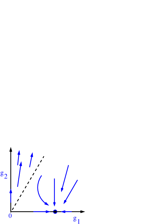
Figure 2: (Color online)Schematic flow lines in the $g_{1}-g_{2}$ plane. Small filled circle (blue) marks the stable FP ($2\epsilon/5,0$). The broken (nonuniversal) line is a schematic demarcation between the region controlled by the stable FP (corresponding to a flat membrane) and the region where flow lines point towards infinity, signalling breakdown of a flat membrane.

Let us now consider the consequence of negative $\kappa_{e}=\kappa_{R}(q\sim 2\pi/L)<0$ possible for sufficiently large $B^{2}$, for a membrane of size $L$. Keeping the dominant corrections we obtain at 2d,

$$\kappa_{e}-\kappa\approx\frac{3}{8}(\frac{A}{\kappa}-\frac{2B^{2}}{\kappa^{2}})\int_{2\pi/L}^{\Lambda}\frac{d^{2}q_{1}}{(2\pi)^{2}q_{1}^{4}}.$$ (8)

A membrane with a size larger than $\xi$ can no longer remain flat and destabilizes or crumples for $\kappa_{e}(L=\xi)=0$, yielding (neglecting terms $O(1/\Lambda^{2})$ which are small for $\xi\gg 1/\Lambda$)

$$\frac{3K_{B}T\xi^{2}}{128\pi^{3}}\left[A\left(\kappa_{0}-\frac{\chi^{2}}{2\mu+\lambda}\right)-\frac{8\chi^{2}\mu^{2}}{(\lambda+2\mu)^{2}}\right]$$ (9)

$$= -\left(\kappa_{0}-\frac{\chi^{2}}{2\mu+\lambda}\right)^{3},$$

where an explicit factor of $K_{B}T$ has been inserted in (9). Thus, $\xi\rightarrow\infty$ as $\chi^{2}\rightarrow\chi_{L}^{2}$, a lower threshold where

$$\chi_{L}^{2}=\frac{A\kappa_{0}(2\mu+\lambda)^{2}}{A(2\mu+\lambda)+8\mu^{2}}=\frac{\kappa_{0}(2\mu+\lambda)}{1+\frac{2\mu}{\mu+\lambda}}.$$ (10)

For $\chi^{2}>\chi_{L}^{2}$, $\kappa_{e}(\xi)=0$, leading to destabilization of the flat membrane and its crumpling at scales larger than $\xi$. On the other hand, $\xi\rightarrow 0$ as $\chi^{2}\rightarrow\chi_{U}^{2}=\kappa_{0}(2\mu+\lambda)$, such that for $\chi^{2}>\chi_{U}^{2}$, the membrane crumples at all scales. Unsurprisingly, $\chi_{U}^{2}$ is same as obtained from Eq. (3) above; clearly $\chi_{U}^{2}>\chi_{L}^{2}$ with none of them having any $T$-dependence. For $\chi^{2}<\chi_{L}^{2}$, a flat membrane ensues in TL. See Fig. 3 for a schematic phase diagram in the $\chi-\kappa_{0}$ plane.

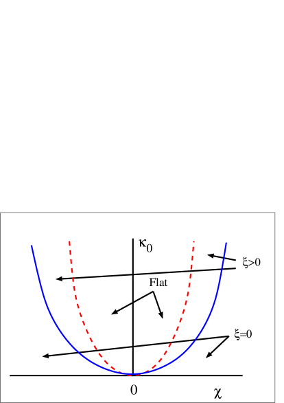
Figure 3: (Color online) Schematic phase diagram in the $\chi-\kappa_{0}$ plane. The red, inner parabola (broken line) and the blue, outer parabola (continuous line) represent, respectively, $\chi^{2}=\chi_{L}^{2}$ and $\chi^{2}=\chi_{U}^{2}$. In the region $\chi_{L}^{2}<\chi^{2}<\chi_{U}^{2}$, the membrane becomes unstable for a length $L>\xi$ (finite), the persistence length. Inside the inner parabola, $\xi\rightarrow\infty$ and the membrane always remains flat. Beyond the outer parabola ($\chi^{2}>\chi_{U}^{2}$), the membrane no longer remains flat at any $L$ (see text).

Furthermore from Eq. (9), $\xi=\sqrt{\frac{128\pi^{3}\kappa^{3}}{K_{B}T(6B^{2}-3A\kappa)}}$, yielding $\xi\propto 1/\sqrt{T}$ over a relevant range of $T$.

Consider now the mean spontaneous curvature $\langle C_{0}\rangle$ in the different regimes delineated by $\chi$. For $\chi^{2}<\chi_{L}^{2}$, a flat membrane ensues in the long wavelength limit, and $\langle C_{0}\rangle=0$; see AP. This is consistent with a statistically flat membrane in TL. In contrast, for $\chi^{2}>\chi_{L}^{2}$, $\langle C_{0}\rangle=\langle({\boldsymbol{\nabla}}h)^{2}\rangle\chi/\kappa_{0}=\int_{2\pi/L}^{\Lambda}\frac{d^{2}q}{(2\pi)^{2}}q^{2}\langle|h({\bf q})|^{2}\rangle\chi/\kappa_{0}$ clearly diverges for $L>\xi$. Thus, the crumpling instability is generically associated with a diverging spontaneous curvature.

A finite surface tension $\sigma$, if present, will control the long wavelength fluctuations of the membrane surface-tension . We note that $\sigma$ receives no relevant fluctuation corrections from the nonlinear terms $A$ and $B$ in (4). Interestingly however, for a sufficiently large $\chi^{2}$, $\kappa_{e}$ that dominates at the intermediate wavevectors, may become negative, leading to finite wavevector instabilities, a feature testable in controlled in-vitro experiments.

Although a full RBC alberts is clearly symmetric under inversion (since the two lipid bilayers are identical in structure), each bilayer clearly has an asymmetric environment having the spectrin network only on one (inner) side of it. Following the logic outlined above, our theory can be readily extended to two identical lipid membranes confining a spectrin network, that may serve as a minimal model for a whole RBC. Using symmetry arguments as above, one can construct a coarse-grained free energy. An analysis similar to the one above indicates towards statistical flatness of RBC membranes for sufficiently low spectrin-lipid interaction strength, beyond which crumpling of the RBC should be observed. Details will be considered elsewhere tb-future . Recent studies on live RBC membranes joanny1 ; joanny2 reveal enhanced fluctuations in the RBC membranes for low frequencies. While a live RBC membrane is an active or driven system, and hence outside the scope of our theory, any consistent hydrodynamic theory for live RBC membranes should reduce to our theory in its equilibrium limit. Our theory reveals the crumpling instability induced by strong enough asymmetry ($\chi^{2}>\chi_{U}^{2}$) in a flat membrane. It must be generalized to study the nature of the thermodynamically stable structurally crumpled state ($\chi^{2}>\chi_{U}^{2}$). Formal similarities between a direct generalization of our model to study the $T$-driven crumpling transition weinberg ; peliti2 and the standard Landau theory for phase transitions with cubic nonlinearities open up the intriguing possibility of new universal scaling at the second order crumpling transition and also possibly first order crumpling transitions. Nonetheless, how the structural crumpling elucidated here is connected to the well-known thermal crumpling of flat tethered membranes weinberg ; luca still remains unresolved.

Independent of the precise values of the model parameters (which may yet be unknown experimentally), the general form and structure of the phase diagram (3) can be tested in non living (ATP-depleted) RBC membrane extract artificial , or for model asymmetric membranes by binding spectrin to lipids by presenting positive charges to lipid surfaces toole . The binding of the elastic network to the membrane surface may be controlled by proteins, e.g., Stomatin grzybek ; see also  hendrich for other spectrin-lipid interactions. In laboratory-based controlled in-vitro experiments, the spectrin-lipid membrane interactions, modeled by $\chi$ here, may be controlled by adding cholesterol abhijit in artificially prepared samples, or in ATP-removed RBC membranes. Numerical simulations of the analogous discrete models of asymmetric tethered membranes, similar to the studies in Refs. md-tethered ; mcs ; peng , should be employed to verify our results.

Our assumptions of a fixed distance between the elastic network and the attached lipid membrane is clearly an idealization; for an RBC membrane $l_{0}\sim 30\,nm$ is the average distance between the two safran . Small fluctuations in $l_{0}$ about its mean, expected in ATP-depleted RBC membranes, is not expected to modify our results in any significant manner; see AP for details. Self-avoidance, ignored here for a putative flat membrane, may be important in the unstable phase weinberg . Recent studies on thin, spherical shells indicate that large enough shells can be crushed by thermal effects nelson-new . How the compressibility-mean curvature coupling introduced here affect this result may be investigated in future. The geometric nonlinearities associated with the Monge gauge are irrelevant (in a scaling/RG sense) and hence have been neglected. We have used a planar geometry for simplicity. In other relevant geometries, e.g., spherical (significant for an RBC membrane), there is a nonzero mean spontaneous curvature even without any fluctuation that characterizes the global shape of the membrane. Whether an asymmetric (i.e., one-sided) coupling of a spherical membrane with a spectrin network, described via an analog of the $\chi$-term in (1), either increases or decreases the mean spontaneous curvature may now depend upon whether the spectrin layer is attached to the inner or outer surface of the spherical membrane. How that plays out in regard to the instabilities elucidated above is an important question that should be studied separately. We expect our work to provide new impetus towards detailed experimental studies of asymmetric tethered membranes.

Acknowledgement:- TB and AB gratefully acknowledge partial financial support from the Alexander von Humboldt Stiftung, Germany under the Research Group Linkage Programme (2016).

APPENDIX (AP)

I Calculation of ${\mathcal{F}}_{h}$ for the full non-linear theory

We integrate over $u_{ij}$ to obtain an effective free enrgy that depends only on $h$. We proceed by breaking $u_{ij}$ into $q$-dependent and $q$-independent parts; ${\bf q}$ being a wave-vector, $q=|{\bf q}|$.

$$u_{ij}(x) = u_{ij}^{0}+A_{ij}^{0}+\Sigma_{q\neq 0}[\frac{i}{2}(q_{j}u_{i}(q)+q_{i}u_{j}(q))+A_{ij}(q)]\exp(i{\bf q}.{\bf x}),$$ (11)

where $A_{ij}(q)=\frac{1}{2}\int d^{2}x\exp(-i{\bf q}.{\bf x})(\nabla_{i}h)(\nabla_{j}h)$, ${\bf x}$ is a $2d$ Cartesian displacement vector. We now use the fact that any $2d$ symmetric second rank tensor can be written as a sum of transverse and longitudinal parts. Let $\phi(q)=\frac{q_{i}q_{j}}{q^{2}}A_{ij}$. We can write

$$A_{ij} = \frac{q_{i}q_{j}}{q^{2}}\phi+A_{ij}-\frac{q_{i}q_{j}q_{m}q_{n}}{q^{4}}A_{mn}$$ (12)

$$= \frac{q_{i}q_{j}}{q^{2}}\phi+P_{ij}\Phi,$$

where, $P_{ij}=\delta_{ij}-\frac{q_{i}q_{j}}{q^{2}}$ and $P_{ij}\Phi=[\delta_{mi}\delta_{nj}-\frac{q_{i}q_{j}q_{m}q_{n}}{q^{4}}]A_{mn}$. Thus $P_{ij}P_{ij}\Phi=\Phi=P_{ij}A_{ij}$. We now write $A_{ij}$ as a combination of longitudinal and transverse parts :

$$A_{ij}=\frac{1}{2}(q_{i}\theta_{j}+q_{j}\theta_{i})+P_{ij}\Phi,$$ (13)

where the first term in the rhs represents the longitudinal component of $A_{ij}$ and $P_{ij}\Phi$ gives the transverse part. Here $\theta_{i}=\frac{q_{i}\phi}{q^{2}}$. Thus in real space, we can write $u_{ij}=\frac{1}{2}(\nabla_{i}\tilde{u}_{j}+\nabla_{j}\tilde{u}_{i})+P_{ij}\Phi$, where $\tilde{u}_{i}(x)=u_{i}(x)+\theta_{i}(x)$. Taking only the $u$-dependent part in ${\mathcal{F}}$, we have

$$I=\int d^{2}x[\frac{\lambda}{2}u_{ii}^{2}+\mu u_{ij}u_{ij}+\chi u_{ii}\nabla^{2}h].$$ (14)

Now $\int d^{2}xu_{ij}u_{ij}=\int d^{2}r[\frac{1}{4}(\nabla_{i}\tilde{u}_{j}+\nabla_{j}\tilde{u}_{i})^{2}+(P_{ij}\Phi)^{2}]$. Also, $\int d^{2}xu_{ii}u_{jj}=\int d^{2}x[(\nabla_{i}\tilde{u}_{i})^{2}+2\Phi\nabla_{i}\tilde{u}_{i}+\Phi^{2}]$ and $\int d^{2}x(P_{ij}\Phi)^{2}=\int d^{2}x\Phi^{2}$. We now write $\tilde{u}_{i}=\tilde{u}_{i}^{L}+\tilde{u}_{i}^{T}$, where $\tilde{u}_{i}^{L}$ and $\tilde{u}_{i}^{T}$ represent the longitudinal and transverse components of $\tilde{u}_{i}$, respectively. Since $\tilde{u}_{i}^{L}$ is fully longitudinal, we can write $\tilde{u}_{i}^{L}=\nabla_{i}\psi$, where $\psi$ is a scalar. This implies

$$\int d^{2}x(\nabla_{i}\tilde{u}_{j}^{L})^{2} = \int d^{2}x(\nabla_{i}\nabla_{j}\psi)(\nabla_{i}\nabla_{j}\psi)=\int(\nabla_{i}^{2}\psi)(\nabla_{j}^{2}\psi)$$ (15)

$$= \int d^{2}x(\nabla_{i}\tilde{u}_{i}^{L})^{2}$$

Using these values, we have

$$I=\int d^{2}x[\frac{\lambda}{2}[(\nabla_{i}\tilde{u}_{i})^{2}+2\Phi\nabla_{i}\tilde{u}_{i}+\Phi^{2}]+\mu[(\nabla_{i}\tilde{u}_{i}^{L})^{2}+(\nabla_{i}\tilde{u}_{j}^{T})^{2}+\Phi^{2}]+\chi(\nabla_{i}\tilde{u}_{i}^{L}+\Phi)\nabla^{2}h]$$ (16)

We note that the coupling between $u_{ij}$ and $h$ appears only in the form of $\tilde{u}_{i}^{L}$ and thus $u_{i}^{T}$ may be integrated out trivially. After proper recombination of terms in Eq. (16) of AP, we get

$$I = \int d^{2}x[(\lambda/2+\mu)[(\nabla_{i}\tilde{u}_{i}^{L})+\frac{\lambda\Phi}{\lambda+2\mu}+\frac{\chi\nabla^{2}h}{\lambda+2\mu}]^{2}-\frac{\lambda^{2}\Phi^{2}}{2\lambda+4\mu}$$ (17)

$$- \frac{\chi^{2}(\nabla^{2}h)^{2}}{2\lambda+4\mu}-\frac{\lambda\chi\Phi(\nabla^{2}h)}{\lambda+2\mu}+(\lambda/2+\mu)\Phi^{2}+\chi\Phi\nabla^{2}h]$$

Integrating over $\tilde{u}_{i}^{L}$, we arrive at the following equation

$$I=\int d^{2}x[\frac{\mu(\mu+\lambda)}{\lambda/2+\mu}\Phi^{2}+\chi(\nabla^{2}h)\Phi\frac{\mu}{\lambda/2+\mu}-\frac{\chi^{2}(\nabla^{2}h)^{2}}{2(2\mu+\lambda)}]$$ (18)

Using Eq. (18) above and the value of $\Phi$, we arrive at the free energy ${\mathcal{F}}_{h}$ of the main text.

II Interacting Gaussian and mean curvatures

Noting that (see, e.g., Ref. [1] of the main text)

$$-\nabla^{2}[\frac{1}{2}P_{ij}(\nabla_{i}h)(\nabla_{j}h)]=\det\left(\nabla_{i}\nabla_{j}h\right),$$ (19)

yields $P_{ij}(\nabla_{i}h)(\nabla_{j}h)=\int d^{d}x^{\prime}M(|{\bf x}-{\bf x}^{\prime}|)S({\bf x}^{\prime})$, where $S({\bf x})$ is the local Gaussian curvature at $\bf x$, $M(|{\bf x}|)$ is the inverse Fourier transform of $1/q^{2}$. Then,

$$\int d^{d}x\nabla^{2}hP_{ij}(\nabla_{i}h)(\nabla_{j}h)=\int d^{d}xd^{d}x^{\prime}\nabla^{2}h({\bf x})M(|{\bf x}-{\bf x}^{\prime})S({\bf x}^{\prime}).$$ (20)

In particular, at $2d$, $M(|{\bf x}|)\sim\ln x$, establishing the picture that the $B$-term in the free energy ${\mathcal{F}}_{h}$ of the main text may be interpreted as interacting mean and Gaussian curvatures via long range interactions.

III One-loop Feynman diagrams

The one-loop Feynman diagrams which contribute to the fluctuation corrections of $\kappa,A$ and $B$ are shown in Fig. 5, Fig. 6 and Fig. 7 of AP, respectively.

Figure 4: One-loop Feynman diagram that originates from the $A$-nonlinear term and contributes to the fluctuation corrections of $\kappa$.

Figure 5: One-loop Feynman diagrams that originate from the $B$-nonlinear term and contribute to the fluctuation corrections of $\kappa$.

Figure 6: One-loop Feynman diagram contributing to fluctuation corrections of $A$.

Figure 7: One-loop Feynman diagram contributing to fluctuation corrections of $B$.

IV Discrete recursion relations

After rescaling of wave-vectors ${\bf q}$ via ${\bf q}^{\prime}=b{\bf q}$ and the field $h({\bf q})=\zeta_{h}h^{\prime}({\bf q}^{\prime})$; $\zeta_{h}=b^{(d+4-\eta)/2}$, $\eta$ being the anomalous dimension of $h({\bf q})$

$$\kappa^{\prime} = b^{-\eta}\kappa[1+(\frac{AK_{d}}{\kappa^{2}}-\frac{2B^{2}K_{d}}{\kappa^{3}})\int_{\Lambda/b}^{\Lambda}\frac{d^{d}q}{(2\pi)^{d}q^{4}}]$$

$$A^{\prime} = b^{-2\eta+4-d}A[1-\frac{AK_{d}}{2\kappa^{2}}\int_{\Lambda/b}^{\Lambda}\frac{d^{d}q}{(2\pi)^{d}q^{4}}]$$

$$B^{\prime} = b^{\frac{-3\eta+4-d}{2}}B[1-\frac{AK_{d}}{2\kappa^{2}}\int_{\Lambda/b}^{\Lambda}\frac{d^{d}q}{(2\pi)^{d}q^{4}}].$$ (21)

The discrete recursion relations in terms of the coupling constants $g_{1}$ and $g_{2}$ are given by :

$$g_{1}^{\prime} = \frac{A^{\prime}K_{d}}{(2\pi)^{d}\kappa^{\prime 2}}=b^{\epsilon}g_{1}[1-(\frac{5g_{1}}{2}-4g_{2})\int_{\Lambda/b}^{\Lambda}\frac{d^{d}q}{q^{4}}]$$

$$g_{2}^{\prime} = \frac{B^{\prime 2}K_{d}}{(2\pi)^{d}\kappa^{\prime 3}}=b^{\epsilon}g_{2}[1-(4g_{1}-6g_{2})\int_{\Lambda/b}^{\Lambda}\frac{d^{d}q}{q^{4}}]$$ (22)

V Spontaneous curvature and odd order correlators of $h$

Upon rescaling $h$ by $\sqrt{\kappa}$, free energy ${\mathcal{F}}_{h}$ of the main text can be written as

$${\mathcal{F}}_{h}=\int d^{d}r[(\nabla^{2}h)^{2}+(2\pi)^{d}\frac{g_{1}}{4}(P_{ij}\nabla_{i}h\nabla_{j}h)^{2}+(2\pi)^{d}g_{2}\nabla^{2}h(P_{ij}\nabla_{i}h\nabla_{j}h)],$$ (23)

in $d$-dimensions. The $g_{2}$-term in (23) violates the inversion symmetry. At the stable RG FP, $g_{2}=0$, rendering (23) symmetric under inversion of $h$. Mean spontaneous curvature $\langle C_{0}\rangle$ clearly scales with $g_{2}$ in the effective, long wavelength renormalized theory, and hence vanishes in the flat phase in the long wavelength limit. Thus, in the renormalized theory all odd order correlators of the form $\langle h({\bf q}_{1})h({\bf q}_{2})h({\bf q}_{3})....h({\bf q}_{n})\rangle,\,{\bf q}_{1}+{\bf q}_{2}+{\bf q}_{3}+...+{\bf q}_{n}=0$ ($n>0$ an odd integer) vanish. Hence, the equilibrium states of an asymmetric nearly flat membrane that is thermodynamically stable is in fact identical to their symmetric counterparts in asymptotic long wavelength limit. The equilibrium states of an asymmetric tethered membrane in the unstable phase for $\chi^{2}>\chi_{L}^{2}$ are of course very different from their symmetric counterparts.

VI Effect of fluctuating membrane-network distance

In the main text, we have considered a fixed distance $l$ between the lipid membrane and the spectrin network. In a realistic situation, the distance $l$ should be a fluctuating quantity; see Fig. 8. In live RBCs, the average spacing $\langle l\rangle\sim 30nm$ and is of the same order of magnitude as the root mean squared fluctuation amplitude of the lipid membrane distance . This should make the fluctuation of $l$ significantly affect the fluctuation of the lipid membrane in a live RBC. For an ATP-depleted RBC or an artificial system of spectrins deposited on a lipid bilayer, the root mean squared fluctuation amplitude of the lipid membrane should be small ($\ll\langle l\rangle$), and hence, should be irrelevant. We demonstrate this in a simple model calculation below.

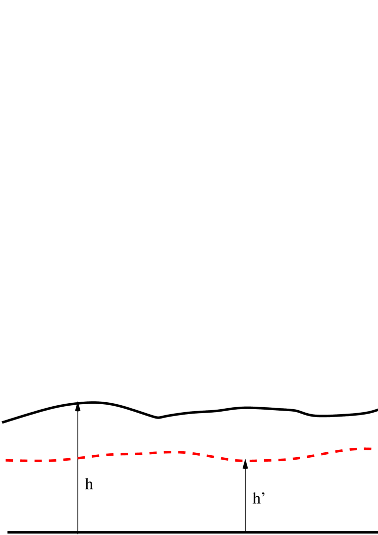
Figure 8: Schematic side view of the lipid membrane (black continuous line) of height $h({\bf r})$ and the spectrin network (broken red line) of height $h^{\prime}({\bf r}^{\prime})$, measured with respect to a Monge gauge base plain (black straight line); $h({\bf r})-h^{\prime}({\bf r})=l({\bf r})\neq const.$ (see text).

We start with a simple model free energy

$${\mathcal{F}}_{hh^{\prime}}=\int d^{2}r[\frac{\kappa_{0}}{2}(\nabla^{2}h)^{2}+\frac{\lambda}{2}u_{ii}^{2}+\mu u_{ij}^{2}+\tilde{A}g(h-h^{\prime}).$$ (24)

Here, $g(h-h^{\prime})$ models the inter-membrane (i.e., between the lipid bilayer and the spectrin network) potential; this is a nonuniversal function, and depends on the detailed interactions of the specific lipid molecules and spectrin filaments. Nonetheless, on simple physical grounds, we impose $g(h-h^{\prime})=0$ for $h=h^{\prime}$ (no interaction potential when the two superpose), and $g(h-h^{\prime})=0$ again for $h-h^{\prime}\rightarrow\infty$. We expect $g(h-h^{\prime})$ to have one minimum at an intermediate distance that is the preferred distance $l$ between the lipid bilayer and the spectrin network; for live RBCs, $l\sim 30nm$ distance . Parameter $\tilde{A}$ is a function of any quantity that is tilt-invariant; this models the fact that the the magnitude of the intermembrane potential not only depends on the local distance between the two, but also on the local configurations the lipid membrane and spectrin bilayer, which are modeled by $\tilde{A}$. In the limit when the lipid bilayer is completely decoupled from the spectrin network, $g(h-h^{\prime})=0$ identically.

At a finite temperature $T$, there should be fluctuations in the local distance about the preferred distance; the extent of fluctuations should depend on the depth and sharpness of the potential well (potential minimum). In a long wavelength approximation, choose

$$\tilde{A}=\alpha_{1}u_{ii}\nabla^{2}h+\alpha_{2}u_{ii}\nabla^{2}h^{\prime},$$ (25)

where we have ignored possible dependences of $\tilde{A}$ on $u_{ij}^{2}$,or its linear dependences on $\nabla^{2}h,\nabla^{2}h^{\prime}$ (and any of their products), as these do not affect the line of arguments outlined below; $\alpha_{1},\alpha_{2}$ are phenomenological constants. In the fixed distance limit, $h-h^{\prime}=l_{0}$ (a const.), $g(h-h^{\prime})=a_{1}l_{0}$ for small $l_{0}$, $a_{1}$ is another phenomenological constant. With this, ${\mathcal{F}}_{hh^{\prime}}$ in (24) immediately yields the free energy $\mathcal{F}$ in the main text [Eq. (1) in the main text] with the identification $\chi=(\alpha_{1}+\alpha_{2})a_{1}l_{0}$.

We now generalize by allowing small fluctuations in the distance $l$ about $l_{0}$. Let $h({\bf r})-h^{\prime}({\bf r})=l=s({\bf r})+l_{0}\neq const.$, $\langle s({\bf r})\rangle=0$, is a fluctuating quantity. Small fluctuations of $l({\bf r})$ implies $\sqrt{\langle s({\bf r})^{2}\rangle}\ll l_{0}$. For small fluctuations, we write

$$g(h-h^{\prime})=g(l_{0}+s({\bf r}))\approx g(l_{0})+\gamma s({\bf r}),$$ (26)

where $\gamma$ is a phenomenological constant that we set to unity below without any loss of generality. In that case, in terms of $h^{\prime}$, the local strain tensor $u_{ij}$ is given by

$$u_{ij} = \frac{1}{2}[\partial_{i}u_{j}+\partial_{j}u_{i}+(\partial_{i}h^{\prime})(\partial_{j}h^{\prime})]$$ (27)

$$= \frac{1}{2}[\partial_{i}u_{j}+\partial_{j}u_{i}+(\partial_{i}h)(\partial_{j}h)-\partial_{i}h\partial_{j}s-\partial_{i}s\partial_{j}h+\partial_{i}s\partial_{j}s].$$

Further assume $\langle s({\bf r})s(0)\rangle=D\delta({\bf r})$. This is a reasonable assumption, given that there are no long-range microscopic fluctuating degrees of freedom expected to be present in thermal equilibrium. This implies $C_{s}=\langle|s({\bf q}|^{2}\rangle=(2\pi)^{d}D$, a finite constant even in the infra-red limit (wavevector ${\bf q}\rightarrow 0$). Compare this with the bare correlator of $h$, $C_{h}=\langle|h({\bf q}|^{2}\rangle=1/(\kappa q^{4})$, that diverges in the limit ${\bf q}\rightarrow 0$. Averaging over $s$ then yields additional diagrams which correct $\kappa,\,A$ and $B$. These diagrams have exactly the same form as the corresponding one-loop diagrams in the fixed distance limit; see Fig. 5, Fig. 6 and Fig. 7, respectively, except that one or more internal lines in the new diagrams now correspond to $C_{s}$. Since $C_{s}$ is a constant, whereas $C_{h}$ is infra-red divergent, all the new diagrams are subleading (in a scaling/RG sense) to the corresponding diagrams Fig. 5, Fig. 6 and Fig. 7, respectively. Thus, no new relevant corrections are generated.

If we consider the instability due to asymmetry at a finite scale $\xi$, then the additional one-loop contributions to $\kappa,\,A,\,B$ that are generated after averaging over $s$ can shift the threshold on $\chi^{2}$ for the instability (or, the vanishing of $\kappa_{e}$). However, the qualitative picture remains unchanged. We, therefore, conclude that small fluctuations in the membrane-elastic network does not affect our results in the main text, obtained with the assumption of a fixed distance, in any significant manner.

References

- (1) Statistical Mechanics of Membranes and Surfaces, edited by D. Nelson, T. Piran, and S. Weinberg World Scientific, Singapore (1989).
- (2) Pontes B, Ayala Y, Fonseca ACC, Romão LF, Amaral RF, Salgado LT, et al. (2013) Membrane Elastic Properties and Cell Function. PLoS ONE 8(7): e67708. doi:10.1371/journal.pone.0067708
- (3) F. Giess et. al, Biophys. J., 87, (2004).
- (4) J. R. C. Whyte and S. Munro, Journal of Cell Science, 115, 2627 (2002).
- (5) K. J. Wiese Eur. Phys. J. B, 1, 269 (1998).
- (6) F. F. Abraham, W. E. Rudge and M. Plischke, Phys. Rev. Lett. 62 15 (1989).
- (7) Y. Kantor et al, Phys. Rev. A 35 3056 (1987).
- (8) D. Moldovan and L. Golubovic Mat. Res. Soc. Symp. Proc., 543 (1999).
- (9) Eva-K Sinner and W. Knoll, Current Opinion in Chemical Biology, 5, 705 (2001).
- (10) T. Betz et al, Proc. Natl Acad. Sci. USA 106, 15320 (2009).
- (11) H. Turlier et al, em Nature Phys. 12, 513 (2016).
- (12) P. M. Chaikin and T. C. Lubensky, Principles of condensed matter physics, (Cambridge University Press, Cambridge 2000).
- (13) E. Guitter et al, J. Phys. France 50, 1787 (1989).
- (14) L. Peliti and S. Leibler, Phys. Rev. Lett. 54, 1690 (1985).
- (15) I. Lopez-Montero, R. Rodriguez-Garcia and F. Monroy, J. Phys. Chem. Lett. 3, 1583 (2012).
- (16) T. Auth, S. A. Safran and N. S. Gov, Phys. Rev. E 76, 051910 (2007).
- (17) B. Alberts, D. Bray, J. Lewis, M. Raff, K. Roberts, J.D. Watson, Molecular Biology of the Cell, 3rd edition (Garland, New York, 1994).
- (18) We ignore any random attachment-detachment of the spectrin layer with the lipid membrane as those are believed to be of nonequilibrium origin; see, e.g. Refs. joanny1 ; joanny2 above.
- (19) We do not distinguish between and . Their differences in the Monge gauge contribute to corrections higher order in and are ignored here in the long wavelength limit.
- (20) D. R. Nelson and L. Peliti, J. Physique 48, 1085 (1987).
- (21) This is quantitatively different from the RG results on symmetric tethered membranes, see, e.g., Ref. chaikin . We believe that this quantitative difference is due to different -dimensional generalization of the theory.
- (22) A clear signature of surface tension in an RBC remains controversial till date; see, e.g., W. Choi, J. Yi and Y. W. Kim, Phys. Rev. E 92, 012717 (2015).
- (23) T. Banerjee and A. Basu, work in progress.
- (24) P. J. O’Toole, I. E. G. Morrison and R. J. Cherry, Biochimica et Biophysica Acta - Biomembranes, Elsevier 1466 39 (2000).
- (25) M. Grzybek et. al, Chemistry and Physics of Lipids, 141, 133 (2006).
- (26) A. B. Hendrich, K. Michalak, M. Bobrowska and A. Kozubek, Gen. Physiol. Biophys., 10, 333 (1991)
- (27) M. Mitra, A. Patra and A. Chakrabarti, Eur. Biophys. J. 44, 635 (2015).
- (28) Z. Peng et. al, Proc Natl Acad Sci U S A, 110, 33 (2013).
- (29) A. Kosmrlj and D. Nelson, arXiv:1606.06750.

References

- (1) A. Ziker, H. Engelhardt and E. Sackmann, J. Phys. (Paris) 48, 2139 (1987); B. S. Bull, R. S. Weinstein and R. A. Korpman, Blood Cells 12, 25 (1986); V. Heinrich et al, Biophys. J. 81, 1452 (2001); G. Popescu et al, J. Biomed. Opt. Lett., 10, 060503 (2005).