Correlations between critical parameters and bulk properties of nuclear matter.

Abstract

The present work starts by providing a clear identification of correlations between critical parameters ($T_{c}$, $P_{c}$, $\rho_{c}$) and bulk quantities at zero temperature of relativistic mean-field models (RMF) presenting third and fourth order self-interactions in the scalar field $\sigma$. Motivated by the nonrelativistic version of this RMF model, we show that effective nucleon mass ($M^{*}$) and incompressibility ($K_{o}$), at the saturation density, are correlated with $T_{c}$, $P_{c}$, and $\rho_{c}$, as well as, binding energy and saturation density itself. We verify agreement of results with previous theoretical ones regarding different hadronic models. Concerning recent experimental data of the symmetric nuclear matter critical parameters, our study allows a prediction of $T_{c}$, $P_{c}$ and $\rho_{c}$ compatible with such values, by combining them, through the correlations found, with previous constraints related to $M^{*}$ and $K_{o}$. An improved RMF parametrization, that better agrees with experimental values for $T_{c}$, is also indicated.

I Introduction

One of the most successfully methods to treat strongly interacting matter at the hadronic level is QHD (Quantum HadroDynamics) qhd . In this quantum field theory, that adequately incorporates effects of quantum mechanics and relativity, nucleons are described by the Dirac spinor $\psi$, and the exchanged mesons by $\sigma$ and $\omega$ fields, responsible to take into account the attractive and repulsive nature, respectively, of nuclear interaction. The nuclear saturation is obtained in this model by the near cancellation of the scalar and vector potentials, written in terms of the $\sigma$ and $\omega$ mean-field values. By using this type of treatment, many effective models have been constructed in order to better describe infinite nuclear matter and finite nuclei properties. The starting model was initially developed by Walecka in the seventies walecka . This seminal work was followed by many other improved versions, and several variations (parametrizations) were built. For a collection of such models, see for instance, Refs. rmf ; bali1 .

Concerning these particular relativistic mean-field (RMF) models, a specific and detailed study on the possible correlations presented by the bulk parameters they describe, and how (under what conditions) they can emerge, has not yet been completed. Many investigations were performed showing indications or trends of correlations, but clear conditions on what physical parameters are important to generate such trends are not totally established. In that direction, we have developed investigations on the subject in Ref. bianca , and verified that, for the RMF model described by the Lagrangian density presenting only the $\sigma^{3}$ and $\sigma^{4}$ terms for scalar meson self-interaction, the effective nucleon mass plays an important role on the arising of correlations between bulk quantities in both isoscalar and isovector sectors. For the latter sector, for instance, we have shown bianca how symmetry energy bali2 ; bali3 ; bali4 ; bali5 ; bali6 ; fred correlates with its next order bulk parameters, namely, slope and curvature. In this work, we proceed to further investigate these possible correlations, but now analyzing the finite temperature regime of the RMF model presenting $\sigma^{3}$ and $\sigma^{4}$ self-interactions. We study here how the critical parameters ($T_{c}$, $P_{c}$, $\rho_{c}$) of this model can correlate with zero temperature bulk quantities, such as effective mass and incompressibility. In order to perform such an analysis, we first use the analytical structure of the nonrelativistic version of this RMF model to predict correlations of $T_{c}$, $P_{c}$ and $\rho_{c}$ with bulk parameters at $T=0$. The details of these calculations are presented in Sec. II. In Sec. III, we show how correlations of RMF model emerges, motivated by results presented in the previous section. We also compare our findings with theoretical results of former investigations kapusta ; lattimer ; natowitz ; rios , and with available experimental values concerning $T_{c}$, $P_{c}$ and $\rho_{c}$ of infinite symmetric nuclear matter natowitz ; karn1 ; karn2 ; karn3 ; karn4 ; karn5 ; elliott . We show which parametrizations are compatible with experimental data, by combining the critical parameters values with other bulk parameters constraints, such as one related to the effective nucleon mass. Finally, in Sec. IV, we provide a summary and the main conclusions of our work.

II Nonrelativistic analysis

In order to analyze possible correlations of the critical density, temperature and pressure of neutron-proton symmetric nuclear matter, we investigate a particular nonrelativistic model, namely, the nonrelativistic limit (NRL) of the relativistic nonlinear point-coupling (zero range) model with self-interactions in the $\bar{\psi}\psi$ condensate until fourth order. As pointed out in previous studies bianca , the model generated from this NRL exhibits many explicit correlations among zero temperature bulk quantities, and can also be used as a starting point to search the same correlations in finite range RMF parametrizations presenting self-interactions in the scalar field ($\sigma$), also until fourth order. In the following, we present the formalism and construction of the main equations of state of this NRL model.

II.1 Formalism at zero temperature

In nuclear physics, point-coupling (or zero range) models assume that nucleons interact with each other only when they are in contact - a zero interaction range means there is no meson exchanges between protons and neutrons. From a qualitative point of view, since the nuclear interaction range is inversely proportional to the mesons mass, one can consider a point-coupling model as one in which the mesons mass are high enough (infinity), leading to a vanishing nuclear range.

In nonrelativistic frameworks, the most known and used point-coupling model is the Skyrme one skyrme , successfully used in description of infinite nuclear matter and finite nuclei. In relativistic contexts, on the other hand, nonlinear relativistic point-coupling (NLPC) models have been applied nlpc2 ; nlpc3 ; nlpc4 ; newrefpc1 ; newrefpc2 ; nlpc1 ; sulaksono ; pclambda to extract nuclear ground-state observables, with results comparable in quality to those obtained by usual relativistic finite range models. Here, we use the point-coupling version of the finite-range RMF model presenting terms of $\sigma^{3}$ and $\sigma^{4}$ (we discuss this particular model in the next section). Its Lagrangian density, for symmetric neutron-proton system and in the zero temperature regime, is given by

$$\mathcal{L}_{\mbox{\tiny NLPC}} = \bar{\psi}(i\gamma^{\mu}\partial_{\mu}-M)\psi-\frac{1}{2}G^{2}_{\mbox{\tiny V}}(\bar{\psi}\gamma^{\mu}\psi)^{2}+\frac{1}{2}G^{2}_{\mbox{ \tiny S}}(\bar{\psi}\psi)^{2}$$ (1)

$$+ \frac{A}{3}(\bar{\psi}\psi)^{3}+\frac{B}{4}(\bar{\psi}\psi)^{4}.$$

The Euler-Lagrange equation applied to $\bar{\psi}$ in Eq. (1) gives rise to the following Dirac equation for the $\psi$ field,

$$(i\gamma^{\mu}\partial_{\mu}-M+G^{2}_{\mbox{\tiny S}}\rho_{s}-\gamma^{0}G^{2}_{\mbox{\tiny V}}\rho+A\rho_{s}^{2}+B\rho_{s}^{3})\psi=0,\quad\,\,\,$$ (2)

with $\rho_{s}=\bar{\psi}\psi$. Here, $\rho$ is the nucleon density. The nonrelativistic limit of the NLPC model sulaksono is then obtained by first writing the large component $\phi$ of the Dirac field $\psi$ in terms of the small one $\chi$. This procedure leads to

$$(\boldsymbol{\sigma\cdot k}\,\tilde{B}\,\boldsymbol{\sigma\cdot k}\,+\,M+S+V)\phi = E\phi$$ (3)

with

$$\tilde{B} = \frac{\tilde{B}_{0}}{1+(\epsilon-S-V)\tilde{B}_{0}}\,\simeq\,\tilde{B}_{0}+\tilde{B}_{0}^{2}(S+V-\epsilon),$$ (4)

being $\tilde{B}_{0}=1/[2(M+S)]$, and $\epsilon=E-M$. The vector and scalar potentials are, respectively, $V=G^{2}_{\mbox{\tiny V}}\rho$ and $S=-G^{2}_{\mbox{\tiny S}}\rho_{s}-A\rho_{s}^{2}-B\rho_{s}^{3}$. By using in Eq. (3) the approximation (4), and taking into account an expansion up to order $(k/M)^{2}$, one can derive the following single-particle energy,

$$H = \frac{k^{2}}{2M^{*}}+(G^{2}_{\mbox{\tiny V}}-G^{2}_{\mbox{\tiny S}})\rho-A\rho^{2}-B\rho^{3}$$ (5)

where the density dependence of the nucleon effective mass $M^{*}$ reads

$$M^{*}(\rho)=\frac{M^{2}}{(M+G^{2}_{\mbox{\tiny S}}\rho+2A\rho^{2}+3B\rho^{3})}.$$ (6)

In the calculations, we have also used that the scalar density can be approximated by $\rho_{s}=\rho(1-2\tilde{B}_{0}k^{2})$.

From the single-particle energy in Eq. (5), we conclude that the energy of a system of $N$ nucleons is

$$E_{N}=\frac{2}{M^{*}}\sum_{i=0}^{k_{F}}k_{i}^{2}+N[(G^{2}_{\mbox{\tiny V}}-G^{2}_{\mbox{\tiny S}})\rho-A\rho^{2}-B\rho^{3}],$$ (7)

where $k_{F}$ is the Fermi momentum and, due to the Pauli exclusion principle, $4$ is the number of nucleons in each energy level. By assuming in one dimension the momentum discretization as $k=\frac{2\pi n}{L}$ (periodic conditions), we have

$$\sum_{i=0}^{k_{F}}k_{i}^{2}=\frac{L}{2\pi}\sum_{i=0}^{k_{F}}\frac{2\pi}{L}\,k_{i}^{2}=\frac{L}{2\pi}\sum_{i=0}^{k_{F}}\Delta k\,k_{i}^{2}.$$ (8)

In the continuum limit ($\Delta k\rightarrow 0$) we have

$$\sum_{i=0}^{k_{F}}k_{i}^{2}\rightarrow\frac{L}{2\pi}\int_{0}^{k_{F}}k^{2}\,dk.$$ (9)

Thus, in three dimensions,

$$\sum_{i=0}^{k_{F}}k_{i}^{2} \rightarrow \frac{V}{(2\pi)^{3}}\int k^{2}\,d^{3}k=\frac{V}{2\pi^{2}}\frac{k_{F}^{5}}{5}=\frac{3V\lambda}{20}\rho^{\frac{5}{3}},\quad$$ (10)

where $\lambda=(3\pi^{2}/2)^{\frac{2}{3}}$ and $V=L^{3}$ is the system volume. By applying such analysis to Eq. (7), we can finally write the system energy density, $\varepsilon=E_{N}/V$, as

$$\varepsilon^{\mbox{\tiny(NR)}} = \frac{3\lambda}{10M^{*}}\rho^{\frac{5}{3}}+(G^{2}_{\mbox{\tiny V}}-G^{2}_{\mbox{\tiny S}})\rho^{2}-A\rho^{3}-B\rho^{4}.$$ (11)

From Eq. (11) it is possible to obtain all remaining thermodynamical quantities of the system. For our purposes in this paper, we will focus on the expression for the pressure, calculated as $P=\rho^{2}\frac{\partial(\mathcal{E}/\rho)}{\partial\rho}$. Its form is the following,

$$P^{\mbox{\tiny(NR)}} = (G^{2}_{\mbox{\tiny V}}-G^{2}_{\mbox{\tiny S}})\rho^{2}-2A\rho^{3}-3B\rho^{4}$$ (12)

$$+ \frac{\lambda}{5M^{2}}\left(M+\frac{5}{2}G^{2}_{\mbox{\tiny S}}\rho+8A\rho^{2}+\frac{33}{2}B\rho^{3}\right)\rho^{\frac{5}{3}}.\quad$$

For other equations of state derived from the NRL model, including those of the isovector sector, such as the one for symmetry energy, its slope and curvature, we address the reader to Ref. bianca .

The coupling constants of the model are $G^{2}_{\mbox{\tiny S}}$, $G^{2}_{\mbox{\tiny V}}$, $A$, and $B$. They are adjusted in order for the model to present particular values of $\rho_{o}$ (saturation density), $B_{o}$ (binding energy), $K_{o}$ (incompressibility) and $M^{*}_{o}$, with the last three quantities evaluated at $\rho=\rho_{o}$. This is done by solving a system of four equations, namely, $\varepsilon^{\mbox{\tiny(NR)}}(\rho_{o})=-B_{o}$, $K^{\mbox{\tiny(NR)}}(\rho_{o})=9[\partial P^{\mbox{\tiny(NR)}}/\partial\rho]_{\rho_{o}}=K_{o}$, $P^{\mbox{\tiny(NR)}}(\rho_{o})=0$, and $M^{*}(\rho_{o})/M=M^{*}_{o}/M\equiv m^{*}$. Following such a procedure, we are able to construct different parametrizations of the NRL model, using as input physical values of the observables $\rho_{o}$, $B_{o}$, $K_{o}$ and $m^{*}$.

II.2 Finite temperature regime: critical parameters and correlations

As a first comment on the calculations in the finite temperature regime, we remind the reader that in any fermion system with a four-fermion interaction, namely, a contact one as in NLPC model or a boson-mediated as in the model we will discuss in the next section, there are various zero-sounds in scalar, spin and spin-isospin channels, which do not contribute to the ground state at zero temperature, but do so at finite temperatures. For the sake of simplicity and as a first approximation, such contributions will be disregarded in the present calculations but can be, in principle, important.

In order to investigate possible correlations in the finite temperature regime of the NRL model, we proceed to include temperature effects in Eq. (12) by adding the classical ideal gas contribution $\rho T$ as a first approximation, i.e, neglecting any quantum fluctuations. This term was inspired by the work of Ref. mekjian . Despite this very crude approximation, one can verify from Fig. 1 that the model still presents the qualitative patterns exhibited by hadronic models at finite temperatures around $T\lesssim 20$ MeV temp1 ; temp2 ; temp3 ; temp4 ; temp5 ; temp6 ; temp7 ; rios ; temp8 ; temp9 , i.e., the van der Waals-like isotherms at different temperatures with the respective spinodal points (points in which $\partial P^{\mbox{\tiny(NR)}}/\partial\rho=0$).

Figure 1: Some isotherms of the NRL model constructed for a parametrization in which $\rho_{o}=0.15$ fm^-3, $B_{o}=16$ MeV, $K_{o}=250$ MeV, and $m^{*}=0.6$.

We also see a critical behavior at a temperature after which the system shows only a gaseous nuclear matter phase. This critical temperature, $T=T_{c}$, characterizes the system’s critical point (CP), with thermodynamic coordinates $\rho=\rho_{c}$ and $P=P_{c}$. As another feature, it is worth noticing that all isotherms are confined to a region where the densities are always lower than $\rho_{o}$, indicating that the liquid-gas phase transition occurs always at subsaturation densities, a feature shared by all the usual hadronic models.

In the particular parametrization used in Fig. 1, we see that the value of the critical temperature lies around $12$ MeV. We highlight that such value also depends on the way the equations of state are obtained. In our calculation we are using the mean-field approximation. In other approaches, such as the chiral perturbation theory, accounting for the inclusion of loop contributions leads to a change of $T_{c}$ to higher values. In Ref. fritsch , for instance, a three-loop calculation of nuclear matter produced $T_{c}=25.5$ MeV.

Still concerning the CP, where $P=P_{c}$ at the critical density ($\rho_{c}$) and temperature ($T_{c}$), it also satisfies the condition of vanishing first and second derivatives in the $P\times\rho$ function. Therefore, in order to exactly locate the CP, it is necessary to impose, simultaneously, the following conditions,

$$P_{c}=P(\rho_{c},T_{c}),\quad\frac{\partial P}{\partial\rho}\bigg{|}_{\rho_{c},T_{c}}=0,\quad\frac{\partial^{2}P}{\partial\rho^{2}}\bigg{|}_{\rho_{c},T_{c}}=0.\quad$$ (13)

For the NRL limit, these conditions lead to the three equation given by

$$2(G^{2}_{\mbox{\tiny V}}-G^{2}_{\mbox{\tiny S}})-12A\rho_{c}-36B\rho_{c}^{2}$$

$$+\frac{2\lambda}{9M^{2}}\left(M+10G^{2}_{\mbox{\tiny S}}\rho_{c}+\frac{352}{5}A\rho_{c}^{2}+\frac{2541}{10}B\rho_{c}^{3}\right)\rho_{c}^{-\frac{1}{3}}=0,$$ (14)

$$T_{c} =-2(G^{2}_{\mbox{\tiny V}}-G^{2}_{\mbox{\tiny S}})\rho_{c}+6A\rho_{c}^{2}+12B\rho_{c}^{3}$$

$$-\frac{\lambda}{3M^{2}}\left(M+4G^{2}_{\mbox{\tiny S}}\rho_{c}+\frac{88}{5}A\rho_{c}^{2}+\frac{231}{5}B\rho_{c}^{3}\right)\rho_{c}^{\frac{2}{3}},$$ (15)

and

$$P^{\mbox{\tiny(NR)}}_{c} =(G^{2}_{\mbox{\tiny V}}-G^{2}_{\mbox{\tiny S}})\rho_{c}^{2}-2A\rho_{c}^{3}-3B\rho_{c}^{4}+\rho_{c}T_{c}$$

$$+\frac{\lambda}{5M^{2}}\left(M+\frac{5}{2}G^{2}_{\mbox{\tiny S}}\rho_{c}+8A\rho_{c}^{2}+\frac{33}{2}B\rho_{c}^{3}\right)\rho_{c}^{\frac{5}{3}}.$$ (16)

One can see that, except for $\rho_{c}$, all critical parameters have an analytical form well defined. Thus, for $T_{c}$ and $P_{c}$, it is possible to search for functional forms relating them to zero temperature bulk quantities. In order to proceed in that direction, we need to write the coupling constants of the NRL model, $G^{2}_{\mbox{\tiny S}}$, $G^{2}_{\mbox{\tiny V}}$, $A$, $B$, as a function of $\rho_{o}$, $B_{o}$, $K_{o}$ and $m^{*}$. This calculation was already performed in Ref. bianca . It is straightforward to implement it in Eqs. (15) and (16). However, we still need to find out how $\rho_{c}$ depends on $\rho_{o}$, $B_{o}$, $K_{o}$ and $m^{*}$. In order to perform such analysis, we first fix the saturation density and binding energy values to those well established in the literature, namely, $\rho_{o}=0.15$ fm^-3 and $B_{o}=16$ MeV, to specifically search for the function $\rho_{c}=\rho_{c}(K_{o},m^{*})$. Following this route, we numerically solve Eq. (14) and present in Fig. 2 the results of $\rho_{c}$ as a function of $K_{o}$ for different values of $m^{*}$.

Figure 2: Critical density of the NRL model as a function of incompressibility for different effective mass values.

As shown in Fig. 2, the critical density is much more sensitive to variation of the incompressibility than of the effective mass. Furthermore, the $K_{o}$ variation is practically linear. From this result, it is possible to parametrize the $K_{o}$ dependence of $\rho_{c}$ as follows,

$$\rho_{c}=\alpha+\beta K_{o},$$ (17)

with $\alpha=(0.0278\pm 1.34\times 10^{-4})$ fm^-3, and $\beta=(6.84\times 10^{-5}\pm 4.76\times 10^{-7})$ MeV^-1 fm^-3. Thus, the use of this $\rho_{c}(K_{o})$ function in Eq. (15), along with the expressions of $G^{2}_{\mbox{\tiny S}}$, $G^{2}_{\mbox{\tiny V}}$, $A$ and $B$ as a function of $\rho_{o}$, $B_{o}$, $K_{o}$ and $m^{*}$, leads to the following analytical expressions for $T_{c}$,

$$T_{c} =a_{0}(\alpha+\beta K_{o})^{\frac{2}{3}}+\sum_{n=1}^{6}\frac{a_{n}}{t}(\alpha+\beta K_{o})^{m}(t_{n1}K_{o}+t_{n2})$$

$$-\frac{1}{m^{*}}\sum_{n=1}^{6}\frac{b_{0}}{t}b_{n}(\alpha+\beta K_{o})^{m}.$$ (18)

In this expression, $m=n$ for $n\leqslant 3$, and $m=n-7/3$ for $n>3$. One also has that $t=3M^{2}-19E_{\mbox{\tiny F}}^{o}M+18E_{\mbox{\tiny F}}^{o2}$, with $E_{\mbox{\tiny F}}^{o}=3\lambda\rho_{o}^{\frac{2}{3}}/10M$. The coefficients are listed in the Appendix. It is worth to notice that in order for $T_{c}$ to be given in MeV, we need to convert $\alpha$ and $\beta$ to appropriate units. Such a conversion leads to $\alpha=(59.8\pm 10.1)^{3}$ MeV³ and $\beta=(22.9\pm 1.91)^{2}$ MeV². In these units, the densities are given in MeV³.

Following the same procedure in Eq. (16), we also found an analytical form for the critical pressure in the NRL model. The result is,

$$P_{c} =c_{0}(\alpha+\beta K_{o})^{\frac{5}{3}}+\sum_{n=1}^{6}\frac{c_{n}}{t}(\alpha+\beta K_{o})^{l}(t_{n1}K_{o}+t_{n2})$$

$$-\frac{1}{m^{*}}\sum_{n=1}^{6}\frac{d_{0}}{t}d_{n}(\alpha+\beta K_{o})^{l},$$ (19)

where $l=n+1$ for $n\leqslant 3$, and $l=n-4/3$ for $n>3$. For complete expressions of the coefficients, including its $\rho_{o}$ and $B_{o}$ dependence, we address the reader to the Appendix. The incompressibility dependence of $T_{c}$ and $P_{c}$ is displayed in Fig. 3 for some fixed values of $m^{*}$.

Figure 3: Critical (a) temperature, and (b) pressure of the NRL model as a function of incompressibility for different effective mass values.

As we see in Fig. 3, $T_{c}$ and $P_{c}$, as well as $\rho_{c}$ are increasing functions of the incompressibility. On the other hand, critical temperature and pressure are more sensitive to effective mass effects than the critical density. Furthermore, $T_{c}$ and $P_{c}$ are also increasing functions of $m^{*}$. In next section, we will verify if such patterns are also exhibited in RMF models.

III RMF parametrizations analysis

III.1 Theoretical framework

In the original Walecka model walecka , there are two free parameters adjusted to impose the values of two particular observables of infinite nuclear matter, namely, $\rho_{o}$ ($\sim 0.15$ fm^-3) and $B_{o}$ ($\sim 16$ MeV). However, the model fails in the description of the incompressibility and effective mass ratio ($m^{*}=M^{*}/M$) at the saturation density, for the results for their values lie close to $550$ MeV and $0.54$, respectively. In order to solve that problem, Boguta and Bodmer boguta have introduced in the original Walecka model two additional terms representing cubic and quartic self-interactions in the $\sigma$ field, providing two new free parameters now adjusted to correctly reproduce $K_{o}$ and $m^{*}$. The Lagrangian density of the Boguta-Bodmer (BB) model is,

$$\mathcal{L} =\overline{\psi}(i\gamma^{\mu}\partial_{\mu}-M)\psi+g_{\sigma}\sigma\overline{\psi}\psi+\frac{1}{2}(\partial^{\mu}\sigma\partial_{\mu}\sigma-m^{2}_{\sigma}\sigma^{2})$$

$$-\frac{\mathcal{A}}{3}\sigma^{3}-\frac{\mathcal{B}}{4}\sigma^{4}-g_{\omega}\overline{\psi}\gamma^{\mu}\omega_{\mu}\psi-\frac{1}{4}F^{\mu\nu}F_{\mu\nu}+\frac{1}{2}m^{2}_{\omega}\omega_{\mu}\omega^{\mu},$$ (20)

with $F_{\mu\nu}=\partial_{\nu}\omega_{\mu}-\partial_{\mu}\omega_{\nu}$. The free parameters are $g_{\sigma}$, $g_{\omega}$, $g_{\rho}$, $\mathcal{A}$ and $\mathcal{B}$.

Since the original work of Boguta and Bodmer boguta published in 1977, many parametrizations of the BB model were proposed along the years. For a list of $128$ of them, collected in a unique reference, we address the reader to Ref. rmf . In the notation of that paper, the authors named the BB parametrization as type 2 ones. Those obtained from the original Walecka model are called type 1 parametrizations.

From Eq. (20), it is possible to construct all thermodynamical quantities at zero and finite temperature by following, for instance, the steps shown in Ref. serot . For our purposes in this paper, we only show the pressure of symmetric ($\gamma=4$) infinite nuclear matter, that reads,

$$P =\dfrac{G_{\omega}^{2}\rho^{2}}{2}-\dfrac{(\Delta M)^{2}}{2G_{\sigma}^{2}}+\dfrac{g_{3}(\Delta M)^{3}}{3}-\dfrac{g_{4}(\Delta M)^{4}}{4}$$

$$+\dfrac{\gamma}{6\pi^{2}}\int_{0}^{\infty}\dfrac{dk\,k^{4}}{(k^{2}+{M^{*}}^{2})^{1/2}}\left[n(k,T,\nu)+\bar{n}(k,T,\nu)\right].$$ (21)

with $\Delta M=M^{*}-M$. The Fermi-Dirac distributions for particles and antiparticles are, respectively,

$$n(k,T,\nu) =\frac{1}{e^{(E^{*}-\nu)/T}+1}\quad\mbox{and}$$

$$\bar{n}(k,T,\nu) =\frac{1}{e^{(E^{*}+\nu)/T}+1},$$ (22)

with $E^{*}=(k^{2}+{M^{*}}^{2})^{1/2}$. The effective mass and chemical potential are given by

$$M^{*} =M+g_{\sigma}\langle\sigma\rangle$$

$$=M-G_{\sigma}^{2}\left[\rho_{s}-g_{3}(\Delta M)^{2}+g_{4}(\Delta M)^{3}\right],$$ (23)

and $\nu=\mu-G_{\omega}^{2}\rho$. The vector and scalar densities are also written in terms of $n$ and $\bar{n}$ as follows,

$$\rho =\dfrac{\gamma}{2\pi^{2}}\int_{0}^{\infty}dk\,k^{2}\left[n(k,T,\nu)-\bar{n}(k,T,\nu)\right],$$

$$\rho_{s} =\dfrac{\gamma}{2\pi^{2}}\int_{0}^{\infty}\frac{dk\,M^{*}k^{2}}{(k^{2}+{M^{*}}^{2})^{1/2}}\left[n(k,T,\nu)+\bar{n}(k,T,\nu)\right].$$ (24)

Finally, the new free parameters present in Eqs. (21), (23), and in definition of $\nu$, are defined in terms of the previous ones as $G_{\sigma}^{2}=\frac{g_{\sigma}^{2}}{m_{\sigma}^{2}}$, $G_{\omega}^{2}=\frac{g_{\omega}^{2}}{m_{\omega}^{2}}$, $g_{3}=\frac{\mathcal{A}}{g_{\sigma}^{3}}$, and $g_{4}=\frac{\mathcal{B}}{g_{\sigma}^{4}}$.

III.2 Correlation of critical parameters

We are now able to search for possible correlations between critical parameters of BB parametrizations. As a starting point, we remark that in Ref. bianca , our results indicate correlations between zero temperature bulk parameters in the NRL model that are also reproduced specifically in the parametrizations of the BB model. As an example, in that paper we found, for the isovector sector of the NRL model, that $L_{o}$ (symmetry energy slope at $\rho_{o}$) is linearly correlated with $J$ (symmetry energy at $\rho_{o}$) for those parametrizations presenting fixed values of $m^{*}$ and $K_{o}$. We also found the same correlation conditions for the BB model. Many other bulk parameters, including those from the isoscalar sector, present such a pattern concerning correlations of the BB model and its nonrelativistic version (the NRL model). In that sense, we have used the NRL model as a guide to investigate correlations in the BB model. Here we proceed in the same direction but now regarding correlations between finite and zero temperature quantities. Based on this discussion and applying the critical condition of Eq. (13), we calculated the critical parameters of the $128$ BB parametrizations of Ref. rmf , in order to see some evidence of correlations. The results are shown in Fig. 4.

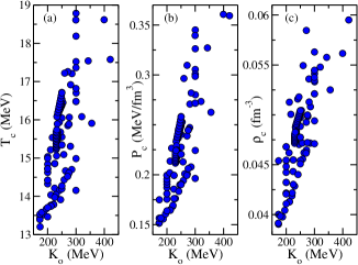
Figure 4: Critical (a) temperature, (b) pressure, and (c) density of the RMF BB parametrizations collected in Ref. rmf .

We see that the critical parameters seem to indicate an increasing trend as $K_{o}$ increases. However, the almost linear pattern exhibited in the NRL parametrizations, or more precisely, a clear connection with $K_{o}$, is not observed, as a simple comparison between Figs. 2 and 3 suggests. Therefore, we proceed to impose the condition of fixed values for $m^{*}$ as we did in the NRL case. In order to perform such analysis, we construct BB parametrizations in which $\rho_{o}=0.15$ fm^-3, $B_{o}=16$ MeV, and for the two remaining observables, namely, $m^{*}$ and $K_{o}$, we investigate models in particular ranges. Actually, here we adopt the same constraints used in Ref. bianca , i.e., for the effective mass ratio, $0.58\leqslant m^{*}\leqslant 0.64$, and for the incompressibility, $250\leqslant K_{o}\leqslant 315$ MeV. According to Ref. ls-splitting , the former constraint allows parametrizations of the BB model to present spin-orbit splittings in agreement with well-established experimental values for ${}^{16}\rm{O}$, ${}^{40}\rm{Ca}$, and ${}^{208}\rm{Pb}$ nuclei. The latter constraint, on the other hand, was generated in a recent study stone where the authors based their calculations on a reanalysis of up-to-date data on isoscalar giant monopole resonance energies of Sn and Cd isotopes. They claimed that such a range, close to the $K_{o}$ value of many RMF parametrizations, was obtained without any microscopic assumptions and is basically due to the suitable treatment of nuclear surface properties. Based on this discussion we show the critical parameters of BB parametrizations in Fig. 5.

Figure 5: Critical parameters of BB parametrizations in which $\rho_{o}=0.15$ fm^-3 and $B_{o}=16$ MeV, for fixed values of $m^{*}$.

We see in Fig. 5(a) that the $K_{o}$ dependence of $T_{c}$ is qualitatively the same as in the NRL model, see Fig. 3(a). The correlation between these quantities is verified for fixed values of the effective mass, with $T_{c}$ being an increasing function of $K_{o}$. The same pattern is also observed for both $P_{c}$ and $\rho_{c}$, as seen in Figs. 5(b) and 5(c), respectively. The behavior of these latter critical parameters was also pointed out by the NRL model, as shown in Figs. 3(b) and 2. For the sake of completeness, we also display in Fig. 6 the effective mass dependence of the critical parameters.

Figure 6: Critical parameters of BB parametrizations in which $\rho_{o}=0.15$ fm^-3 and $B_{o}=16$ MeV, for fixed values of $K_{o}$.

It is verified that they are also tightly correlated. By comparing these results with those from Sec. II, we see that $T_{c}$ and $P_{c}$ of the NRL limit model also depend on $m^{*}$, as in the relativistic case, but $\rho_{c}$ is practically not affected, see Fig. 2. The source of such a difference might be attributed to the fact that, in the NRL model at finite temperature, we did not take into account the $T$ dependence of $\rho$, like in the relativistic case, see Eq. (III.1). If we had done so, we would have $\rho=\rho(E_{kin},T)$ with the kinetic energy $E_{kin}$ being a function of the effective mass, see the first term of Eq. (5). Thus, in the NRL model, the effect of $m^{*}$ on $\rho_{c}$ is underestimated in comparison with the relativistic case.

Based on these results, one can see that most of the correlations present in the NRL model at finite temperature regime, namely, critical parameters related to saturation bulk quantities at zero temperature, are reproduced in the parametrizations of the BB model, since one preserves the same conditions that drive the arising of such correlations. These conditions explain why we do not see a tight correlation of $T_{c}$, $P_{c}$ and $\rho_{c}$ with $K_{o}$, for instance, in the BB parametrizations of Fig. 4. In that case, besides having different values of $\rho_{o}$ and $B_{o}$, each parametrization presents a particular value of effective mass, and do not satisfy the condition of fixed $m^{*}$, constraint that produces a clear connection between the critical parameters and $K_{o}$. Similar analysis can be performed in order to describe the correlation of the critical parameters and $m^{*}$. In this case, it is established if the condition of having BB parametrizations presenting the same value of $K_{o}$ is fulfilled.

Still regarding our findings on the correlations presented here, and in order to clarify our discussion, we remind the reader that they were found for the specific RMF model presenting the self-coupling in the scalar field up to fourth order. We are dealing with parametrizations of the BB model in which the equations of state were obtained through the widely used mean-field approximation (MFA). Therefore, it is not our purpose to classify them as universal. A more detailed study based on other kind of models described by more sophisticated Lagrangian densities in comparison with that of Eq. (20) is in order. Even calculations that go beyond MFA can change the correlations found here, stressing the importance of performing such an investigation in order to establish possible correlations between zero and finite temperature quantities in different kind of hadronic models.

III.3 Comparison with other theoretical studies

Specifically concerning the relation between $T_{c}$ and $K_{o}$, we remark here that our findings for the RMF parametrizations analyzed here are in qualitative agreement with previous studies on such correlation, as we will show in the following. In the Kapusta model of Ref. kapusta , for instance, the author derived an expression for the pressure, based on the Sommerfeld expansion in the degenerate regime (Fermi energy $\gg$ temperature), that reads $P=K_{o}\rho^{2}(\rho-\rho_{o})/9\rho_{o}^{2}+b^{2}M^{*}_{o}\rho^{1/3}T^{2}/6$, with $b=1.809$. This leads to a critical temperature of

$$T_{c}^{\rm K}=0.326\rho_{o}^{1/3}\sqrt{K_{o}/M^{*}_{o}},$$ (25)

with $T_{c}$ being an increasing function of $K_{o}$. In Ref. lattimer , Lattimer and Swesty modified the Kapusta expression for the critical temperature by introducing an opposite dependence of the saturation density, but keeping the increasing pattern concerning $K_{o}$. The correlation reads

$$T_{c}^{\rm LS}=C\rho_{o}^{-1/3}\sqrt{K_{o}},$$ (26)

where $C=0.608$ MeV^1/2 fm^-1. In another study, Natowitz et al. natowitz proposed the inclusion of effective mass effects on the latter correlation, which produced the expression

$$T_{c}^{\rm N}=C^{\prime}\rho_{o}^{-1/3}\sqrt{K_{o}/m^{*}},$$ (27)

with $C^{\prime}=0.484\pm 0.074$ MeV^1/2 fm^-1. Finally in Ref. rios , Rios improved the Kapusta model by introducing, in the pressure equation of state, the density dependence of $M^{*}$ coming from the Skyrme interaction. The result of such improvement generated the following correlation,

$$T_{c}^{\rm R}=0.326\bar{m}^{*}\rho_{o}^{1/3}\sqrt{K_{o}/M},$$ (28)

where $\bar{m}^{*}=m^{*}(\rho=\frac{5\rho_{o}}{12})$. Again, we have here the by now familiar pattern of an increasing $T_{c}$ as a function of $K_{o}$. It is then fair to say that the BB parametrizations share with former hadronic models the qualitative prediction of an increasing $T_{c}$ as $K_{o}$ increases.

Regarding the $T_{c}\times m^{*}$ correlation, the BB parametrizations also show an increasing pattern for $T_{c}$ (and also for $P_{c}$ and $\rho_{c}$). However, the only prediction compatible with such behavior is that from Ref. rios . In that case, $T_{c}^{\rm R}$ increases as $\bar{m}^{*}$ increases, but, for this particular analysis, the correlation is with the effective mass ratio evaluated at a subsaturation density of $\rho=5\rho_{o}/12$, and not exactly at $\rho=\rho_{o}$ as in the case presented in our work.

We have also verified the effect of $K_{o}$ on the critical parameters of the BB model in some known (and largely used) parametrizations of Ref. rmf . The results are depicted in Fig. 7.

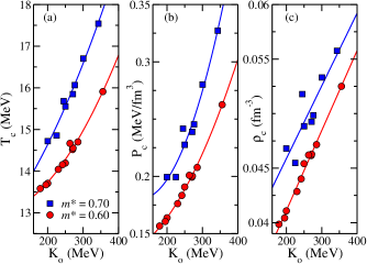
Figure 7: Critical parameters as a function of $K_{o}$ of some BB parametrizations of Ref. rmf presenting $m^{*}=0.60$ (MS2, NL4, NLSH, NLRA1, Q1, NL3, Hybrid, FAMA1, NL-VT1, NL06, NLS) and $m^{*}=0.70$ (S271, P-070, NLM6, NLD, NL07, GM1, GL4, FAMC2). Full lines: fitting curves.

As we can see from this figure, the BB parametrizations present a faster increasing of $T_{c}$ with an increase of $K_{o}$ in comparison with the previous investigations showed by Eqs. (25)-(28). Our results indicate $T_{c}\sim K_{o}^{a}$, with $a\geqslant 1$, different from that pointed out in the aforementioned expressions, namely, $T_{c}\sim K_{o}^{1/2}$. For those parametrizations in which $m^{*}=0.60$, for instance, we found a fitting curve of $T_{c}=13-(1.9\times 10^{-3})K_{o}+(2.9\times 10^{-5})K_{o}^{2}$. In order to become clearer this difference, we plot in Fig. 8 the following ratios

$$r^{\rm K} = \frac{T_{c}}{\rho_{0}^{1/3}\sqrt{K_{0}/M_{0}^{*}}},$$ (29)

$$r^{\rm LS} = \frac{T_{c}}{\rho_{0}^{-1/3}\sqrt{K_{0}}},$$ (30)

$$r^{\rm N} = \frac{T_{c}}{\rho_{0}^{-1/3}\sqrt{K_{0}/m^{*}}},\quad\mbox{and}$$ (31)

$$r^{\rm R} = \frac{T_{c}}{\bar{m}^{*}\rho_{0}^{1/3}\sqrt{K_{0}/M}}.$$ (32)

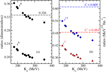
Figure 8: Ratios defined in Eqs. (29)-(32) in comparison with the respective constants presented in Eqs. (25)-(28) for the BB parametrizations of Fig. 7 in which $m^{*}=0.60$.

The comparison of these ratios with the ones derived from Eqs. (25)-(28) shows explicitly the deviations between these different approaches.

By returning to Fig. 7, one notice also some deviations from the fitting curves for those parametrizations presenting $m^{*}=0.70$. We attribute such differences to the distinct values of $\rho_{o}$ and $B_{o}$ presented by each model. For those in which $m^{*}=0.70$, the variation of $\rho_{o}$ and $B_{o}$ is larger than those presenting $m^{*}=0.60$. The former has $\Delta\rho_{o}=0.015$ fm^-3 and $\Delta B_{o}=0.72$ MeV, and the latter, $\Delta\rho_{o}=0.004$ fm^-3 and $\Delta B_{o}=0.69$ MeV. In the BB parametrizations analyzed in Figs. 5 and 6, we did not see any deviation due to the fact that we have fixed the values of saturation density and binding energy, i. e., we had $\Delta\rho_{o}=\Delta B_{o}=0$ in all cases. The effects induced specifically by the variations of $\rho_{o}$ and $B_{o}$ in the critical parameters can be seen in the next Figs. 9 and 10.

Figure 9: Critical parameters as a function of $\rho_{o}$ for $B_{o}=16$ MeV, $m^{*}=0.6$ and $K_{o}=270$ MeV.

Figure 10: Critical parameters as a function of $B_{o}$ for $\rho_{o}=0.15$ fm^-3, $m^{*}=0.6$ and $K_{o}=270$ MeV.

In Fig. 9, we see an increasing effect of $\rho_{o}$ in the critical parameters with a linear dependence in all three quantities. The pattern observed in the critical temperature specifically is also observed in the correlation found in the Kapusta kapusta and Rios rios models, although they have obtained an analytical form of $\rho_{o}^{1/3}$ that differs from the result of the BB parametrizations. In the Lattimer-Swesty and Natowitz models, on the other hand, an opposite effect is found, since now $T_{c}$ is proportional to $\rho_{o}^{-1/3}$, i. e., a decreasing function of saturation density.

In Fig. 10, the increasing pattern is obtained only for $T_{c}$. The two other critical parameters are decreasing functions of $B_{o}$. Furthermore, for the values used in Figs. 9 and 10, we see that $P_{c}$ and $\rho_{c}$ are less sensitive to the variation of $B_{o}$ than of $\rho_{o}$. For a range of around $6\%$ in the central value of $B_{o}=16$ MeV, the changes found in critical pressure and density are $\Delta P_{c}=0.007$ MeV/fm³ and $\Delta\rho_{c}=0.003$ fm^-3, respectively, while a range of around $7\%$ in $\rho_{o}=0.15$ fm^-3 produces $\Delta P_{c}=0.035$ MeV/fm³ and $\Delta\rho_{c}=0.007$ fm^-3, i. e., about five and two times higher variations, respectively. Regarding the critical temperature, $\Delta T_{c}$ is practically the same for the two cases.

III.4 Comparison with experimental data

For a direct application of our findings, we use the correlations exhibited by the BB model to generate parametrizations in which critical parameters can be compared with experimental data reported in different works along the years. Specifically regarding the critical temperature, many studies have been successful in obtaining this quantity. In summary, a beam of relativistic incident light particles that transfers excitation thermal energy ($E^{*}$) is used in order to heat a nucleus. The relationship between $E^{*}$ and $T$ is found through the so called caloric curve. This heating procedure gives rise to different emission processes, namely; gamma rays emission, occurring for $1\lesssim T\lesssim 2$ MeV; nucleon-evaporation, in the range of $2\lesssim T\lesssim 5$ MeV; and multifragmentation, for $T\gtrsim 5$ MeV, this latter process being one that generates emission of $\alpha$ particles, nucleons, and intermediate mass fragments (IMF). Theoretical models are commonly used to fit experimental data of IMF charge distributions by having the critical temperature as a free parameter. Thus, the value of $T_{c}$ is indirectly calculated. In Fig. 11, we compare our theoretical predictions with experimental data obtained for $T_{c}$.

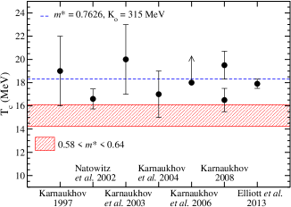
Figure 11: Theoretical predictions (band and dashed line, for $\rho_{o}=0.153$ fm^-3 and $B_{o}=16.32$ MeV) and experimental data (circles) on critical temperature of symmetric nuclear matter. The references are Karnaukhov 1997: karn1 , Natowitz et al. 2002: natowitz , Karnaukhov et al. 2003: karn2 , Karnaukhov et al. 2004: karn3 , Karnaukhov et al. 2006: karn4 , Karnaukhov 2008: karn5 , and Elliott et al. 2013: elliott .

In this figure, the horizontal band bounds the possible values of $T_{c}$ for BB parametrizations presenting effective mass in the range of $0.58\leqslant m^{*}\leqslant 0.64$ ls-splitting , and incompressibility within $250\leqslant K_{o}\leqslant 315$ MeV stone . One can see that such parametrizations are compatible with four experimental points, by taking into account the error bars. However, if we simply discard the constraint related to $m^{*}$, it is possible to construct a BB parametrization in which six (of seven) experimental points are reproduced, including the more recent data on the critical parameters obtained in Ref. elliott where $T_{c}=17.9\pm 0.4$ MeV. In Fig. 11, we indicate by the dashed blue line this specific parametrization presenting $m^{*}=0.7626$ and $K_{o}=315$ MeV. We see that this choice is more compatible with the trend of higher values for $T_{c}$ pointed out by the experimental data.

Finally, concerning critical pressure and density, we have also verified that the constraints on $m^{*}$ and $K_{o}$ produce BB parametrizations presenting the range of $0.19\leqslant P_{c}\leqslant 0.27$ MeV/fm³ and the value of $\rho_{c}=0.05$ fm^-3 (with one significant figure), respectively. By comparing such values with Ref. elliott , that found ranges of $P_{c}=0.31\pm 0.07$ MeV/fm³ and $\rho_{c}=0.06\pm 0.01$ fm^-3 from experimental analysis of compound nuclear and multifragmentation reactions, we found an overlap of around $21\%$ with former range, and agreement within the error bar with the latter one. Moreover, for the parametrization represented in Fig. 11 by the dashed line, where the effective mass constraint is neglected, we found critical pressure and density given, respectively, by $P_{c}=0.34$ MeV/fm³ and $\rho_{c}=0.06$ fm^-3. Notice the very good agreement with the experimental $P_{c}$ and $\rho_{c}$ values from Ref. elliott . As a side remark, we also provide for this parametrization the compressibility factor ($Z_{c}=\frac{P_{c}}{\rho_{c}T_{c}}$), namely, $Z_{c}=0.31$. For the experimental values of critical parameters of Ref. elliott , $Z_{c}=0.29$.

IV Summary and Conclusions

In the present work, we studied correlations between bulk quantities of symmetric nuclear matter at zero temperature and their critical parameters (CP), namely, $T_{c}$, $P_{c}$ and $\rho_{c}$ at finite temperature regime. We performed this analysis in the RMF model presenting nonlinear couplings in the scalar field $\sigma$ up to fourth order, here named the BB (Boguta-Bodmer boguta ) model. The motivation for such an investigation comes from the results (correlations) presented by the nonrelativistic version of the BB model. As in previous works bianca , the correlations presented in the NRL model are reproduced also in the BB one, by imposing the same physical conditions needed to make the relationships arise.

In order to explore in a fully analytical way the NRL model, we proceeded to include the temperature effects in the pressure equation of state by simply adding in Eq. (12) an ideal gas contribution. Such an approximation neglects quantum effects, but still reproduces qualitatively the van der Waals behavior of warm nuclear matter, as displayed in Fig. 1. By imposing the critical conditions of Eq. (13) in the NRL model, we found that $\rho_{c}$, $T_{c}$ and $P_{c}$ are directly correlated with $\rho_{o}$, $B_{o}$, $m^{*}$ and $K_{o}$, as shown by Eqs. (17)-(19). For fixed values of $\rho_{o}$ and $B_{o}$, the results pointed out to an increasing $K_{o}$ dependence of the CP. For $\rho_{c}$, this dependence is verified independently of the effective mass value, see Fig. 2. For $T_{c}$ and $P_{c}$, on the other hand, we verified a positive correlation with $K_{o}$ only for fixed values of $m^{*}$, see Fig. 3. Inspired by these results, we have calculated the CP of the $128$ BB parametrizations of Ref. rmf , looking for possible correlations with bulk quantities at $T=0$. We found a general trend of increasing values of the CP as $K_{o}$ increases, see Fig. 4. Such a trend is confirmed as clear correlations if we choose parametrizations in which the effective mass value is kept fixed, exactly as we have concluded in the NRL model case for $T_{c}$ and $P_{c}$. In Fig. 5 we showed this analysis for BB parametrizations constructed with the ranges of $0.58\leqslant m^{*}\leqslant 0.64$ and $250\leqslant K_{o}\leqslant 315$ MeV. The former range ls-splitting ensures BB models presenting spin-orbit splittings within accepted experimental values, and the latter stone was recently proposed from a reanalysis of up-to-date data on isoscalar giant monopole resonance energies.

The comparison of our findings with previous correlations results of Refs. kapusta ; lattimer ; natowitz ; rios , obtained from other hadronic models, pointed out to a qualitative agreement concerning the $T_{c}\times K_{o}$ correlation ($T_{c}$ is an increasing function of $K_{o}$). We also found a clear correlation between the CP and the effective mass if $K_{o}$ of each BB parametrization is kept fixed, see Fig. 6. For the sake of completeness, we also investigated the relationship of the CP with the saturation density and binding energy. Our results showed an increasing behavior of the CP with $\rho_{o}$, in qualitative agreement with the models of Refs. kapusta ; rios . For the case of $B_{o}$, the BB model present $T_{c}\times B_{o}$ as an increasing function, while $P_{c}$ and $\rho_{c}$ exhibit a decreasing dependence, see Figs. 9 and 10, respectively.

A direct comparison of our findings for $T_{c}$ with experimental data collected from Refs. natowitz ; karn1 ; karn2 ; karn3 ; karn4 ; karn5 ; elliott was performed in Fig. 11. By constraining the BB parametrizations to present values of $0.58\leqslant m^{*}\leqslant 0.64$ ls-splitting and $250\leqslant K_{o}\leqslant 315$ MeV stone , we predicted critical temperatures of $14.2\leqslant T_{c}\leqslant 16.1$ MeV, lower than most of the experimental points, but compatible with four (of seven) of them within the error bars. By neglecting the restriction of effective mass, we could construct a BB parametrization presenting $T_{c}=18.3$ MeV, a value closer to the experimental data, including the more recent one of $T_{c}=17.9\pm 0.4$ MeV from Ref. elliott . For such a parametrization, the effective mass is given by $m^{*}\sim 0.76$, a higher value than those from the range $0.58\leqslant m^{*}\leqslant 0.64$, obtained through an analysis of finite nuclei spin-orbit splittings. If we discard this constraint, we can use the correlation between $T_{c}$ and $m^{*}$ to predict new ranges of effective mass. For example, from Fig. 11, we see that the range of $0.64\leqslant m^{*}\lesssim 0.76$ produces critical temperatures compatible with all experimental data. We remind the reader that this procedure indicates higher values for $m^{*}$, apparently not compatible with finite nuclei calculations of Ref. ls-splitting , but within an analysis of the BB model, i. e., a model with only mesonic self-interactions in the attractive scalar field $\sigma$. A more complete study, taking into account more sophisticated RMF models, such as that named “type 4” model in Ref. rmf , is needed in order to verify if the ranges of $m^{*}$ are kept and even to investigate the role played by the effective mass, and other bulk quantities, in possible correlations with the CP. We will address such study in a future work.

As a last remark, we verified in our study, the first one relating CP and bulk quantities at zero temperature of the RMF BB model, that BB parametrizations constrained to $0.58\leqslant m^{*}\leqslant 0.64$ and $250\leqslant K_{o}\leqslant 315$ MeV present values of $0.19\leqslant P_{c}\leqslant 0.27$ MeV/fm³ and $\rho_{c}=0.05$ fm^-3, compatible with experimental values of $P_{c}=0.31\pm 0.07$ MeV/fm³ and $\rho_{c}=0.06\pm 0.01$ fm^-3 of Ref. elliott . The theoretical values can be further improved if we relax the effective mass condition and choose, for instance, $m^{*}\sim 0.76$. In this case, we predicted $P_{c}=0.34$ MeV/fm³ and $\rho_{c}=0.06$ fm^-3 for this particular BB parametrization ($m^{*}=0.7626$ and $K_{o}=315$ MeV).

Appendix A Coefficients of Eqs. (18) and (19)

The coefficients presented in the expression of $T_{c}$, Eq. (18), of the NRL limit model, are given as follows, $a_{n}:$

$$a_{0} =-\frac{\lambda}{3M},\quad a_{1}=a_{2}=a_{3}=2,\quad a_{4}=2\lambda$$ (33)

$$a_{5}=\frac{88\lambda}{5},\quad a_{6} =\frac{77\lambda}{5}.$$ (34)

$b_{n}:$

$$b_{0} =2E_{\mbox{\tiny F}}^{o},\quad b_{1}=-\frac{\left(2M^{2}-19E_{\mbox{\tiny F}}^{o}M+54E_{\mbox{\tiny F}}^{o2}\right)}{3\rho_{o}},$$ (35)

$$b_{2} =-\frac{8M\left(M-6E_{\mbox{\tiny F}}^{o}\right)}{\rho_{o}^{2}},\quad b_{3}=\frac{2M\left(M-10E_{\mbox{\tiny F}}^{o}\right)}{\rho_{o}^{3}},$$ (36)

$$b_{4} =\frac{2\lambda\left(9M^{2}-70E_{\mbox{\tiny F}}^{o}M+120E_{\mbox{\tiny F}}^{o2}\right)}{9ME_{\mbox{\tiny F}}^{o}\rho_{o}},$$ (37)

$$b_{5} =\frac{352\lambda\left(M-6E_{\mbox{\tiny F}}^{o}\right)}{45M\rho_{o}^{2}},\quad b_{6}=-\frac{77\lambda\left(M-10E_{\mbox{\tiny F}}^{o}\right)}{30M\rho_{o}^{3}}.$$ (38)

For the critical pressure, $P_{c}$, showed in Eq. (19) we have, $c_{n}:$

$$c_{0} =-\frac{2\lambda}{15M},\quad c_{1}=1,\quad c_{2}=\frac{4}{3},\quad c_{3}=\frac{3}{2},$$ (39)

$$c_{4}=\frac{5\lambda}{4},\quad c_{5} =\frac{64\lambda}{5},\quad c_{6}=\frac{121\lambda}{10}.$$ (40)

$d_{n}:$

$$d_{0} =E_{\mbox{\tiny F}}^{o},\quad d_{1}=b_{1},\quad d_{2}=\frac{4}{3}b_{2},\quad d_{3}=\frac{3}{2}b_{3},$$ (41)

$$d_{4} =\frac{5}{4}b_{4},\quad d_{5}=\frac{16}{11}b_{5},\quad d_{6}=\frac{11}{7}b_{6}.$$ (42)

The remaining coefficients presented in both expression are, $t_{n1},t_{n2}:$

$$t_{11} =-\frac{M\left(M-4E_{\mbox{\tiny F}}^{o}\right)}{6\rho_{o}},$$ (43)

$$t_{12} =\frac{1}{\rho_{o}}\left[B_{o}\left(9M^{2}-48E_{\mbox{\tiny F}}^{o}M+18E_{\mbox{\tiny F}}^{o2}\right)\right.$$

$$+\left.E_{\mbox{\tiny F}}^{o}M\left(4M-21E_{\mbox{\tiny F}}^{o}\right)\right],$$ (44)

$$t_{21} =\frac{M\left(M-3E_{\mbox{\tiny F}}^{o}\right)}{\rho_{o}^{2}},$$ (45)

$$t_{22} =-\frac{9B_{o}M\left(3M-13E_{\mbox{\tiny F}}^{o}\right)+3E_{\mbox{\tiny F}}^{o}M\left(5M-27E_{\mbox{\tiny F}}^{o}\right)}{\rho_{o}^{2}},$$ (46)

$$t_{31} =-\frac{M\left(M-2E_{\mbox{\tiny F}}^{o}\right)}{\rho_{o}^{3}},$$ (47)

$$t_{32} =\frac{6B_{o}M\left(3M-10E_{\mbox{\tiny F}}^{o}\right)+6E_{\mbox{\tiny F}}^{o}M\left(M-6E_{\mbox{\tiny F}}^{o}\right)}{\rho_{o}^{3}},$$ (48)

$$t_{41} =\frac{M-6E_{\mbox{\tiny F}}^{o}}{9M\rho_{o}},$$ (49)

$$t_{42} =-\frac{B_{o}\left(6M-32E_{\mbox{\tiny F}}^{o}\right)-2M^{2}+52E_{\mbox{\tiny F}}^{o}M/3-36E_{\mbox{\tiny F}}^{o2}}{M\rho_{o}},$$ (50)

$$t_{51} =-\frac{\left(M-3E_{\mbox{\tiny F}}^{o}\right)}{9M\rho_{o}^{2}},$$ (51)

$$t_{52} =\frac{B_{o}\left(3M-13E_{\mbox{\tiny F}}^{o}\right)+E_{\mbox{\tiny F}}^{o}\left(5M/3-9E_{\mbox{\tiny F}}^{o}\right)}{M\rho_{o}^{2}},$$ (52)

$$t_{61} =\frac{M-2E_{\mbox{\tiny F}}^{o}}{6M\rho_{o}^{3}},$$ (53)

$$t_{62} =-\frac{B_{o}\left(3M-10E_{\mbox{\tiny F}}^{o}\right)+E_{\mbox{\tiny F}}^{o}\left(M-6E_{\mbox{\tiny F}}^{o}\right)}{M\rho_{o}^{3}}.$$ (54)

References

- (1) B. D. Serot, Rep. Prog. Phys. 55, 1855 (1992).
- (2) J. D. Walecka, Ann. Phys. 83, 491 (1974).
- (3) M. Dutra, O. Lourenço, S. S. Avancini, B. V. Carlson, A. Delfino, D. P. Menezes, C. Providência, S. Typel, and J. R. Stone, Phys. Rev. C 90, 055203 (2014).
- (4) B.-A. Li, L. W. Chen, C. M. Ko, Phys. Rep. 464, 113 (2008).
- (5) B. M. Santos, M. Dutra, O. Lourenço, and A. Delfino, Phys. Rev. C 90, 035203 (2014); 92, 015210 (2015).
- (6) L. W. Chen, C. M. Ko, and B.-A. Li, Phys. Rev. Lett. 94, 032701 (2005).
- (7) R. Chen, B.-J. Cai, L. W. Chen, B.-A. Li, X.-H. Li, and C. Xu, Phys. Rev. C 85, 024305 (2012).
- (8) C. Xu, B.-A. Li, and L. W. Chen, Phys. Rev. C 82, 054607 (2010).
- (9) O. Hen, B.-A. Li, W.-J. Guo, L. B. Weinstein, and E. Piasetzky, Phys. Rev. C 91, 025803 (2015).
- (10) B. J. Cai and B.-A Li, Phys. Rev. C 93, 014619 (2016).
- (11) R. N. Mishra, H. S. Sahoo, P. K. Panda, N. Barik, and T. Frederico, Phys. Rev. C 92, 045203 (2015).
- (12) J. Kapusta, Phys. Rev. C 29, 1735 (1984).
- (13) J. M. Lattimer, F. D. Swesty, Nucl. Phys. A 535, 331 (1991).
- (14) J. B. Natowitz, K. Hagel, Y. Ma, M. Murray, L. Qin, R. Wada, and J. Wang, Phys. Rev. Lett. 89, 212701 (2002).
- (15) A. Rios, Nucl. Phys. A 845, 58 (2010).
- (16) V. A. Karnaukhov, Phys. At. Nucl. 60, 1625 (1997).
- (17) V. A. Karnaukhov, et al., Phys. Rev. C 67, 011601(R) (2003).
- (18) V. A. Karnaukhov et al., Nucl. Phys. A 734, 520 (2004).
- (19) V. A. Karnaukhov et al., Nucl. Phys. A 780, 91 (2006).
- (20) V. A. Karnaukhov, Phys. At. Nucl. 71, 2067 (2008).
- (21) J. B. Elliott, P. T. Lake, L. G. Moretto, and L. Phair, Phys. Rev. C 87, 054622 (2013).
- (22) T. H. R. Skyrme, Phil. Mag. 1, 1043 (1956).
- (23) J. J. Rusnak and R. J. Furnstahl, Nucl. Phys. A 627, 495 (1997).
- (24) D. G Madland, T. J Bürvenich, J. A Maruhn, P.-G Reinhard, Nucl. Phys. A 741, 52 (2004).
- (25) O. Lourenço, M. Dutra, A. Delfino, and R. L. P. G. Amaral, Int. Jour. Mod. Phys. E, 16, 3037 (2007).
- (26) P. W. Zhao, Z. P. Li, J. M. Yao, and J. Meng, Phys. Rev. C 82, 054319 (2010).
- (27) T. Niksic, D. Vretenar, and P. Ring, Prog. in Part. and Nucl. Phys. 66, 519 (2011).
- (28) B. A. Nikolaus, T. Hoch, and D. G. Madland, Phys. Rev. C 46, 1757 (1992).
- (29) A. Sulaksono, T. Bürvenich, J. A. Maruhn, P.-G. Reinhard, and W. Greiner, Ann. Phys. 308, 354 (2003).
- (30) Y. Tanimura and K. Hagino, Phys. Rev. C 85, 014306 (2012).
- (31) A. L. Goodman, J. I. Kapusta, A. Z. Mekjian, Phys. Rev. C 30, 851 (1984).
- (32) H. Müller and B. D. Serot, Phys. Rev. C 52, 2072 (1995).
- (33) J. B. Silva, O. Lourenço, A. Delfino, J. S. Sá Martins, M. Dutra, Phys. Lett. B 664 246, (2008).
- (34) G.-H. Zhang, W.-Z. Jiang, Phys. Lett. B 720, 148 (2013).
- (35) V. Vovchenko, D. V. Anchishkin, and M. I. Gorenstein, Phys. Rev. C 91, 064314 (2015).
- (36) V. Vovchenko, D. V. Anchishkin, M. I. Gorenstein, and R. V. Poberezhnyuk, Phys. Rev. C 92, 054901 (2015).
- (37) A. Fedoseewand H. Lenske, Phys. Rev. C 91, 034307 (2015).
- (38) J. R. Torres, F. Gulminelli, and D. P. Menezes, Phys. Rev. C 93, 024306 (2016).
- (39) K. Liu and J.-S. Chen, Phys Rev. C 88, 068202 (2013).
- (40) K. Redlich and K. Zalewski, arxiv:1605.09686v1.
- (41) S. Fritsch, N. Kaiser, and W. Weise Phys. Lett. B 545, 73 (2002).
- (42) J. Boguta and A. R. Bodmer, Nucl. Phys. A 292, 413 (1977).
- (43) R. J. Furnstahl and B. D. Serot, Phys. Rev. C 41, 262 (1990).
- (44) R. J. Furnstahl, J. J. Rusnak, B.D. Serot, Nucl. Phys. A 632, 607 (1998).
- (45) J. R. Stone, N. J. Stone, and S. A. Moszkowski, Phys. Rev. C 89, 044316 (2014).