Efficient Valuation of SCR via a Neural Network Approach
Abstract
As part of the new regulatory framework of Solvency II, introduced by the European Union, insurance companies are required to monitor their solvency by computing a key risk metric called the Solvency Capital Requirement (SCR). The official description of the SCR is not rigorous and has lead researchers to develop their own mathematical frameworks for calculation of the SCR. These frameworks are complex and are difficult to implement. Recently, Bauer et al. suggested a nested Monte Carlo (MC) simulation framework to calculate the SCR. But the proposed MC framework is computationally expensive even for a simple insurance product. In this paper, we propose incorporating a neural network approach into the nested simulation framework to significantly reduce the computational complexity in the calculation. We study the performance of our neural network approach in estimating the SCR for a large portfolio of an important class of insurance products called Variable Annuities (VAs). Our experiments show that the proposed neural network approach is both efficient and accurate.
keywords:
Variable annuity , Spatial interpolation , Neural network , Portfolio valuation , Solvency Capital Requirement (SCR)1 Introduction
The Solvency II Directive is the new insurance regulatory framework within the European Union. Solvency II enhances consumer protection by requiring insurers to monitor the risks facing their organization. An integral part of Solvency II is the Solvency Capital Requirement (SCR) that reduces the risk of insurers’ insolvency. SCR is the amount of reserves that an insurance company must hold to cover any losses within a one year period with a confidence level of .
The calculation standards are described in the documents of the Committee of European Insurnace and Occupational Pensions Supervisors (CEIOP) (e.g., (CEIOP, 2011)). The regulation allows insurance companies to use either the standard formula or to develop an internal model based on a market-consistent valuation of assets and liabilities. Because of the imprecise language of the aforementioned standards, many insurance companies are struggling to implement the underlying model and to develop efficient techniques to do the necessary calculations. In (Christiansen and Niemeyer, 2014; Bauer et al., 2012), rigorous mathematical definitions of SCR are provided. Moreover, (Bauer et al., 2012) describes an implementation of a simplified, but approximately equivalent, notion of SCR using nested Monte Carlo (MC) simulations.
The results of the numerical experiments in (Bauer et al., 2012) to find the SCR for a simple insurance product show that the proposed nested MC simulations are too expensive, even for their simplified notion of SCR. Hence, insurance companies cannot directly use the proposed MC approach to find the SCR for their large portfolios of insurance products. In this paper, we propose a neural network approach to be used within the nested MC simulation framework to ameliorate the computational complexity of MC simulations which allows us to efficiently compute the SCR for large portfolios of insurance products. We provide insights into the efficiency of the proposed extension of the MC simulation framework by studying its performance in computing the SCR for a large portfolio of Variable Annuities, a well-known and important class of insurance products.
A VA is a tax-deferred retirement vehicle that allows a policyholder to invest in financial markets by making payment(s) into a predefined set of sub-accounts set up by an insurance company. The investment of the policyholder should be payed back as a lump-sum payment or a series of contractually agreed upon payments over a period of time in the future. VA products provide embedded guarantees that protect the investment of a policyholder in a bear market and/or from mortality risk (TGA, 2013). For a detailed description of VA products and the different types of guarantees offered in these products, see our earlier paper (Hejazi et al., 2015) and the references therein.
Because of the innovative structure of embedded guarantees in VA products, insurance companies have been successful in selling large volumes of these products (IRI, 2011). As a result, VA products are a large portion of the investment market around the globe and big insurance companies have accumulated large portfolios of these products. The embedded guarantees of VA products expose insurers to a substantial amount of market risk, mortality risk, and behavioral risk. Hence, big insurance companies have developed risk management programs to hedge their exposures, especially after the market crash of 2008.
The rest of this paper is organized as follows. In Section 2, we describe the mathematical definition of SCR as well as its simplified, almost equivalent, version described in (Bauer et al., 2012). In Section 3, we describe a modification of the nested simulation approach of (Bauer et al., 2012) that we use to approximate the SCR. Furthermore, we define a simple asset and liability structure that allows us to remove the assets from the required calculation of the SCR for the portfolio. In Section 4, we describe the neural network framework that we use to estimate the one-year probability distribution of liability for the input portfolio of VA products. In Section 5, we compare the efficiency and accuracy of our method to that of a simple nested MC simulation approach. In Section 6, we conclude the paper.
2 Solvency Capital Requirement
A rigorous treatment of SCR111The material in this section is based largely on the discussion in (Bauer et al., 2012). requires the definition of Available Capital (AC) which is a metric that determines the solvency of a life insurer at each point in time. The AC is the difference between the Market Value of Assets (MVA) and Market Value of Liabilities (MVL):
| (1) |
where the subscript denotes the time, in years, at which each variable is calculated.
Assuming the definition (1) of AC, the SCR, under Solvency II, is defined as the smallest amount of AC that a company must currently hold to insure a non-negative AC in one year with a probability of . In other words, the SCR is the smallest amount that satisfies the following inequality.
| (2) |
In practice, it is hard to find the SCR using definition (2). Hence, Bauer et al. use a simpler, approximately equivalent notion of the SCR which is based on the one-year loss, , evaluated at time zero:
| (3) |
where is the one-year risk-free rate. The SCR is then redefined as the one-year Value-at-Risk (VaR):
| (4) |
This is the definition of the SCR that we use in the rest of this paper.
3 Nested Simulation Approach
Given the formulation of equation (4), we can calculate the SCR by first computing the empirical probability distribution of and then computing the -quantile of the calculated probability distribution. We can implement this scheme by the nested simulation approach of (Bauer et al., 2012). In this section, we first outline the nested simulation approach of (Bauer et al., 2012) and then describe our modification of it to make it more computationally efficient.
In the nested simulation approach of (Bauer et al., 2012), summarized in Figure 1, we first generate sample paths that determine the one-year evolution of financial markets. Note that we are only interested in the partial state of the financial markets. In particular, we are only interested in the state of the financial instruments that help us evaluate the asset values and the liability values of our portfolio. Hence, we can generate a sample state of the financial market by drawing one sample from the stochastic processes that describe the value of those financial instruments of interest.
In the nested simulation approach of (Bauer et al., 2012), for each sample path , we use a MC simulation to determine the value , the available capital one year hence. We also calculate via another MC simulation and use that to determine the value of for each sample path via equation (3). The values , can be used to determine the empirical distribution of . In order to estimate the -quantile for as required by the definition of the SCR in equation (4), we can sort the calculated , values in ascending order and choose the element amongst the sorted values as the approximation for SCR.
The nested MC simulation approach of Figure 1 is computationally expensive even for simple insurance contracts (Bauer et al., 2012). The computational complexity of the approach is caused by two factors: 1) The value of can be very large (Bauer et al., 2012). 2) The suggested MC valuation of for each path and , even for a single contract, is expensive and hence does not scale well to large portfolios of insurance products. In this paper, we focus on the latter problem and provide an approach to significantly reduce the cost of computing each and . We also briefly discuss a proposal to address the former. However, we leave a detailed development and analysis of the proposal as future work.
To begin, we briefly outline our proposal for reducing to address the first problem. In the nested simulation approach suggested by (Bauer et al., 2012), to have a good estimation of the empirical probability distribution of , the number of sample paths, , must be large, since the values, are used to approximate the probability distribution of . Consequently, many values are needed to provide a sufficiently accurate approximation. Because a significant number of these values should, intuitively, be very close to each other, we suggest using a data interpolation scheme to reduce the cost associated with the number of sample paths, . To do the interpolation, we first select/generate a small number, , of paths and evaluate for each path . Then, we use the calculated values of the representative paths to interpolate each associated with each path . The choice of the interpolation scheme that should be used depends on the distribution of the generated paths in the space. The variables that define this space are dependent on the sources of randomness in the financial instruments that we use to value our portfolio. In this paper, we use a simple linear interpolation scheme, described in more detail in Section 5, to reduce the running time of our numerical experiments. We postpone a more thorough development and analysis of the interpolation method to a future paper.
Now we turn to the main focus of this paper, a more efficient way to compute for each path and . A key element in computing the value via equation (3) is the calculation of AC values. From (1), we see that the calculation of AC requires a market consistent valuation of assets and liabilities. Insurance companies can follow a mark-to-market approach to value their assets in a straightforward way. However, the innovative and complex structure of insurance products does not allow for such a straightforward calculation of liabilities. In practice, insurance companies often have to calculate the liabilities of insurance products by direct valuation of the cash flows associated with them (direct method (Girard, 2002)). Hence, the difficulty in calculation of SCR is primarily associated with the difficulty in the calculation of liabilities.
As we discuss in detail in (Hejazi et al., 2015), a MC simulation approach, as suggested in (Bauer et al., 2012), to compute the liability of large portfolios of insurance products is very expensive. Furthermore, traditional portfolio valuation techniques, such as the replication portfolio approach (Dembo and Rosen, 1999; Oechslin et al., 2007; Daul and Vidal, 2009) and the Least Squares Monte Carlo (LSMC) method (Cathcart and Morrison, 2009; Longstaff and Schwartz, 2001; Carriere, 1996), are not effective in reducing the computational cost. The computational complexity of these methods for sophisticated insurance products, such as VA, is comparable to, or more than, the computational complexity of MC schemes. Reducing the amount of computation in these methods often requires significant reduction in their accuracy.
Recently, a spatial interpolation scheme (Hejazi et al., 2015; Gan, 2013; Gan and Lin, 2015) has been proposed to reduce the required computation of the MC scheme by reducing the number of contracts that must be processed by the MC method. In the spatial interpolation framework, we first select a sample of contracts in the space in which the insurance products of the input portfolio are defined. The value of interest for each sample contract is evaluated using MC simulation. The outputs of the MC simulations are then used to estimate the value of interest for other contracts in the input portfolio by a spatial interpolation scheme. In (Hejazi and Jackson, 2016), we describe how a neural network approach to the spatial interpolation can not only solve the problem associated with finding a good distance metric for the portfolio but also provide a better balance between efficiency, accuracy, and granularity of estimation. The numerical experiments of (Hejazi and Jackson, 2016) provided insights into the performance of our proposed neural network approach in estimation of Greeks for a portfolio of VA. We show in this paper how a similar neural network approach can be used within the nested MC simulation framework to find the liabilities and subsequently the SCR for an input portfolio of VA products in an efficient and accurate manner.
Of course, other spatial interpolation schemes could be used within the framework described in the last paragraph. However, in this paper we focus only on the neural network approach to show the potential of using a spatial interpolation scheme within the nested MC simulation framework. Exploring the potential of other spatial interpolation schemes within this context may be the subject of future research. Although we are using a neural network similar to the one proposed in (Hejazi and Jackson, 2016), our experiments demonstrate that a naive usage of the neural network framework to estimate the liability values can provide no better computational efficiency than parallel implementation of MC simulations. As we discuss in (Hejazi and Jackson, 2016), the time it takes to train the neural network accounts for a major part of the running time of the proposed neural network framework. Therefore, if we have to train the network from scratch for each realization of the financial markets () to compute the proposed neural network loses its computational superiority compared to a parallel implementation of the MC simulations. To address this problem, in Section 5, we discuss a methodology to use the parameters for a neural network trained to compute the associated with as a good first guess for the parameters for another neural network to compute associated with , for . The proposed methodology is based on the idea that, for two neural networks that are trained under two market conditions that are only slightly different, the optimal choices of neural network parameters are likely very close to each other.
In summary, we suggest to use the extended nested simulation approach of Figure 2 instead of the more standard nested simulation approach of Figure 1 to approximate the value of SCR via equation (4).
In this paper, as mentioned earlier, our focus is on reducing the computational cost of the MC simulations used to calculate the liability of large portfolios of VA. Hence, to focus on the problem of calculating the liabilities and to make the analysis more tractable, we assume that the company has taken a passive approach (i.e., no hedging is involved) and the only asset of the company is a pool of shareholders’ money that is invested in a money market account and hence accrues risk-free interest. We understand that this is a very simple, and probably unrealistic, asset structure model; however, using a more complex asset structure only makes the computation of asset values more time consuming and diverts our attention from the key issue we are focusing on in this paper which is how to improve the efficiency of the computation of the liability values. Moreover, note that we can use the proposed framework to calculate the portfolio liability value of the input portfolio independently of the evaluation of asset values. That is, a more complex model for asset valuation can be inserted into our proposed framework without changing our scheme for improving the efficiency of the computation of liability values.
The assets are adjusted yearly as required. The proposed simple structure of assets allows us to eliminate the assets in the definition of in (3) as follows.
| (5) |
Hence, in our simplified problem, calculating the SCR reduces to the problem of calculating the current liability and the distribution of the liability in one-year’s time.
4 Neural Network Framework
In this section, we provide a brief review of our proposed neural network framework. For a detailed treatment of this approach, in particular the reason behind our choice of network and training method, see our paper (Hejazi and Jackson, 2016).
4.1 The Neural Network
Our proposed estimation scheme is an extended version of the Nadaraya-Watson kernel regression model (Nadaraya, 1964; Watson, 1964). Assuming are the observed values at known locations , our model estimates at a location where is not known by
| (6) |
where is a nonlinear differentiable function and the subscript, , denotes the range of influence of each on the estimated value. The variable is a location dependent vector that determines the range of influence of each pointwise estimator in each direction of feature space of the input data. In our application of interest in this paper, is the MC estimation of liability. The variables , are vectors in representing the attributes of a sample set of representative VA contracts in the space of the input portfolio. The representative VA contracts are selected using a sampling scheme to effectively fill the space in which the input portfolio is defined. The size of the portfolio of representative VA contracts should be much smaller than the input portfolio for the neural network scheme to be efficient. As we discuss in (Hejazi and Jackson, 2016) and in more detail in (Hejazi, 2016), the choice of the representative contracts can affect the performance, in particular the accuracy, of the neural network framework. Hence, it is important to use an appropriate sampling method. We postpone a discussion of the choice of an effective sampling method to a future paper.
We choose to implement our model (6) using a feed-forward neural network (Bishop, 2006; Fister et al., 2016) that allows us to fine-tune our model to find the optimum choices of the values that minimize our estimation error.
As shown in Figure 3, our feed-forward neural network is a collection of interconnected processing units, called neurons, which are organized in three layers. The first and the last layers are, respectively, called the input layer and the output layer. The intermediate layer is called the hidden layer.
The neurons in the first layer provide the network with the feature vector (input values). Each neuron in the input layer represents a value in the set . Each in has the form
| (7) |
where represents the category of categorical attribute for input VA policy , and represents the category of categorical attribute for representative VA policy in the sample. Each in has the form , and each in has the form . In both of these formulas, is the vector containing the numeric attributes of input VA policy , is the vector containing the numeric attributes of representative VA policy in the sample, is a transformation (linear/nonlinear), determined by the expert user, that assumes a value in an interval of length and . The ’s are used to scale the ’s so that each . It is well-known that scaling the variables in this way helps to increase the rate of convergence of the optimization method described in Section 4.2 used to train the neural network. In essence, our choice of input values allows different bandwidths ( values in (6)) to be used for different attributes of VA policies and in different directions around a representative VA contract in the sample.
Since we are interested in calibrating the functions of equation (6), the number of neurons in the output and hidden layer are equal to the number of representative contracts in the sample. The inputs of neuron in the hidden layer are those values of in the input layer that are related to the representative VA policy . In other words, the input values of neuron in the hidden layer determine the per attribute difference of the input VA contract with the representative VA contract using the features . Assuming are the inputs of neuron at the hidden level, first a linear combination of input variables is constructed
| (8) |
where parameters are referred to as weights and parameter is called the bias. The quantity is known as the activation of neuron . The activation is then transformed using an exponential function to form the output of neuron .
The output of neuron in the output layer is the normalized version of the output for neuron in the hidden layer. Hence the outputs of the network, i.e., , represent a softmax of activations in the hidden layer. These outputs can be used to estimate the value of the liability for input VA as , in which is the value of the liability for representative VA policy . In summary, our proposed neural network allows us to rewrite equation (6) as
| (9) |
where vector represents the features in the input layer that are related to the representative VA policy , and vector contains the weights associated with each feature in at neuron of the hidden layer.
4.2 Network Training Methodology
In order to calibrate (train) the network and find the optimal values of weights and bias parameters, we select a small set of VA policies, which we call the training portfolio, as the training data for the network. The objective of the calibration process is to find a set of weights and bias parameters that minimizes the Mean Squared Error (MSE) in estimation of liability values of the training portfolio. In other words, our objective function is
| (10) |
We use an iterative gradient descent scheme (Boyd and Vandenberghe, 2004) to train the network. However, to speed up the training process, we do mini-batch training (Murphy, 2012) with Nestrov’s Accelerated Gradient (NAG) method (Nesterov, 1983). In mini-batch training, in each iteration, we select a small number of training VA policies at random and compute the gradient of the following error function for this batch.
| (11) |
where is the set of indices for the selected VA policies and superscript denotes the iteration number. Instead of updating the weights and biases by the gradient of (11), in the NAG method, we use a velocity vector that increases in value in the direction of persistent reduction in the objective error function across iterations. We use a particular implementation of the NAG method described in (Sutskever et al., 2013). In this implementation of NAG, weights and biases are updated according to the rules
| (12) |
where is the velocity vector, is known as the momentum coefficient and is the learning rate. The momentum coefficient is an adaptive parameter defined by
| (13) |
where is a user defined constant.
Because of the amount of investments and the structure of guarantees in VA products, the liability values can become large. Big liability values can result in big gradient values which produce big jumps in the updates of (4.2). Therefore, to avoid numerical instability, only in the training stage, we normalize the values of in (11), by dividing each value by the range of guarantee values in the input portfolio.
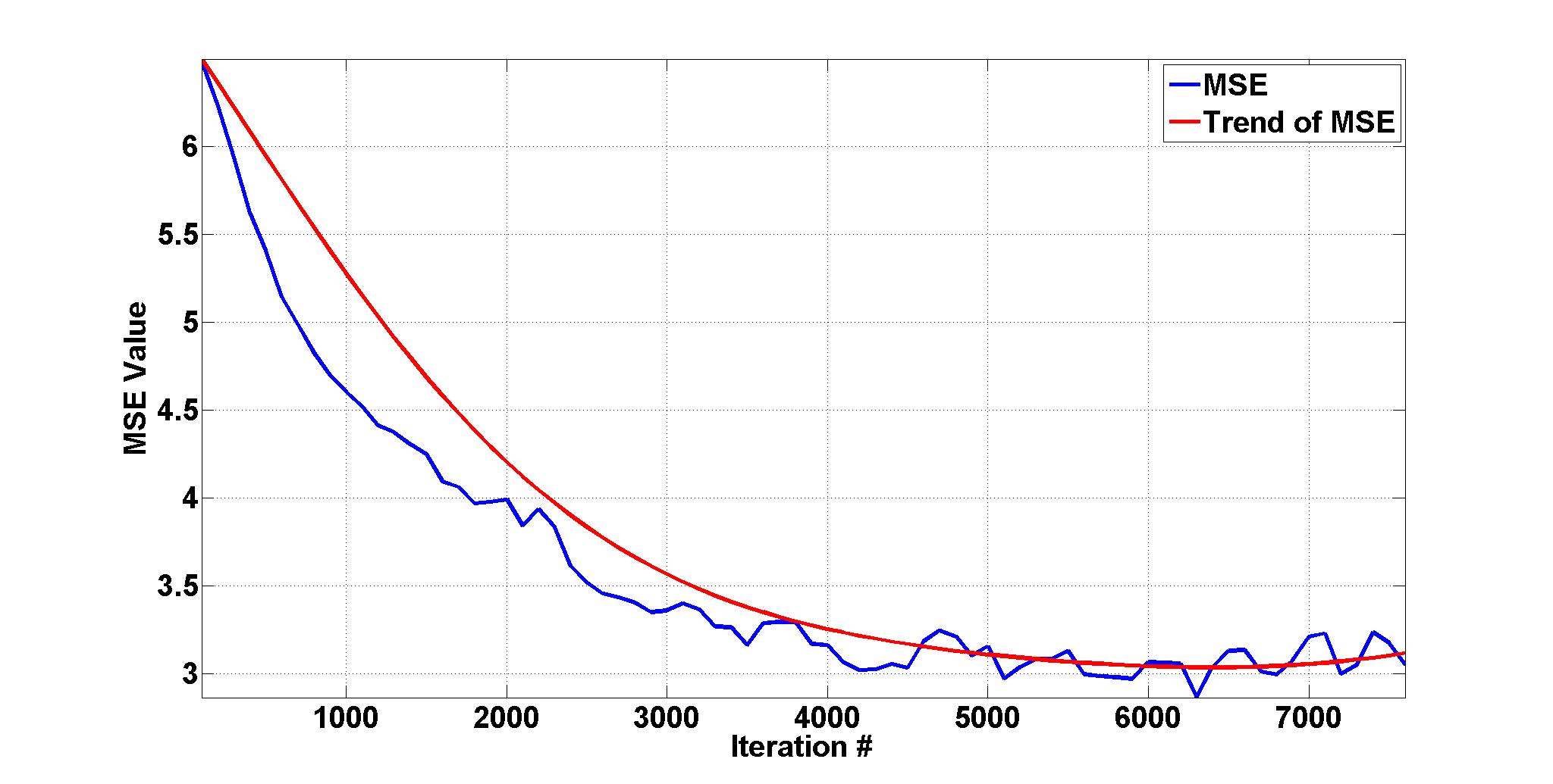
If we allow the network to train for a long enough time, it will start to converge towards a local optimum. Depending on our choice of the representative contracts and the training data, further training of the network after a certain number of iterations might result in overfitting or might not result in significant change in the value of weights and biases, and the associated error. To avoid these pitfalls, we use a set of randomly selected VA policies from the input portfolio as our validation portfolio (Murphy, 2012) and stop the training using a two step verification process. First, we observe if the MSE of the training data drops dramatically or if there is an initial decrease in the MSE of the validation portfolio to a local minimum followed by an increase in the MSE of the validation portfolio. Once any of these events, called stopping events, happens, we train the network for a few more iterations until the mean of the network’s liability estimates for the validation portfolio is within a relative distance of the mean of the MC estimated liability of the validation portfolio via MC simulations or a maximum number of training iterations is reached. The relative distance between the network estimated liablity and the MC estimated liability is calculated as
| (14) |
As shown in the graph of Figure 4, the actual graph of the MSE for the validation portfolio or the training portfolio as a function of iteration number might be volatile. However, a general trend exists in the data. To make the trend clearer, we use a simple moving average with a window of to smooth the data and polynomial fitting of the smoothed data. We detect stopping events using a window of length on the polynomial approximation of the MSE values. A stopping event occurs if the MSE of the validation set has increased in the past recorded values after attaining a minimum. We evaluate the MSE values of the validation set every iteration of the training, to avoid slowing down the training process. , and are user defined parameters and are application dependent.
The neural network outlined above is discussed in more detail in (Hejazi and Jackson, 2016), where we also discuss how to choose the free parameters described above.
5 Numerical Experiments
In this section, we demonstrate the effectiveness of the proposed neural network framework in calculating portfolio liability values in the proposed nested simulation approach of Section 3. To do so, we estimate the SCR for a synthetic portfolio of VA contracts assuming the financial structure of assets as described in Section 3 that allows us to use equation (3).
| Attribute | Value |
|---|---|
| Guarantee Type | {GMDB, GMDB + GMWB} |
| Gender | {Male, Female} |
| Age | |
| Account Value | |
| Guarantee Value | |
| Widthrawal Rate | |
| Maturity |
Each contract in the portfolio is assigned attribute values uniformly at random from the space defined in Table 1. The guarantee values (death benefit and withdrawal benefit) of GMWB riders are chosen to be equal222This is typical of the beginning of the withdrawal phase., but they are different than the account value. The account values of the contracts follow a simple log-normal distribution model (Hull, 2006) with a risk free rate of return of , and volatility of .
We acknowledge that this model of account value is very simple; we use it here to make our computations more tractable. A more complex model increases the number of MC simulations that is required to find liability values and affects the distribution of one-year-time’s liability values. A more complex model of account values may also necessitate the use of more complicated valuation techniques for which the computational complexity is much more than simple MC simulations. However, regardless of the changes imposed by using a more complex model to describe the dynamics of the account value, the proposed nested simulation framework incorporating a neural network approach, described in Sections 3 and 4, can be used to calculate the SCR. Therefore, to focus on our neural network approach in this paper, we have chosen to use a simple account value model to avoid distracting the reader with a lengthy description of a more complex account value model.
A change in the probability distribution of one-year-time’s liability values changes the probability distribution of values. A change in the probability distribution of values can increase the number of sample paths and affect the choice of the interpolation scheme that should be used to calculate the values. As mentioned earlier, in this paper, our focus is not on the choice of the interpolation scheme and/or the size of the sample paths that should be used here. We leave a more thorough study of these questions to future work. We can still repeat the experiments of this section and arrive at the same conclusions even if we directly compute the values for the original paths ; however, the running times will be much bigger.
We can increase the number of MC simulations or use more complex techniques to value liability values. Both of these approaches only slightly increase the running time of our proposed neural network approach to calculate liability values and hence only slightly increase the running time of our proposed nested simulation approach of Section 3. However the aforementioned approaches significantly increase the running time of the nested simulation approach of (Bauer et al., 2012). The nested simulation approach of (Bauer et al., 2012) evaluates the liability values for each VA in the input portfolio; however, our proposed neural network framework only evaluates the liability values for the selected number of sample VA contracts of the representative portfolio, training portfolio, and the validation portfolio and then does a spatial interpolation to find the liability values for the VAs in the input portfolio. Increasing the time to calculate the per VA liability value linearly increases the running time in the nested simulation approach of (Bauer et al., 2012). The size of the representative portfolio, the training portfolio and the validation portfolio combined in practice is much smaller than the size of the input portfolio. Therefore, increasing the time to calculate per VA liability only affects the total running time of the neural network to the extend that the calculation of liability values for the representative portfolio, the training portfolio, and the validation portfolio can affect the training time which in most of our experiments is not significant. Most of the computing time for the neural network approach is consumed in training the network.
We use the framework of (Gan and Lin, 2015) to value each VA contract. Similar to (Hejazi et al., 2015), we use MC simulations to value each contract. In our experiments, we use the mortality rates of the 1996 IAM mortality tables provided by the Society of Actuaries.
We implement our experiments in Java and run them on a machine with dual quad-core Intel X5355 CPUs. For each valuation of the input portfolio using the MC simulations, we divide the input portfolio into 10 sub-portfolios, each with an equal number of contracts, and run each sub-portfolio on one thread, i.e., a total of threads, to value these sub-portfolios in parallel. We use a similar parallel processing approach to value the representative contracts, the training portfolio and the validation portfolio. Although we use the parallel processing capability of our machine for MC simulations, we do not use parallel processing to implement our code for our proposed neural network scheme: our neural network code is implemented to run sequentially on one core. However, there is significant potential for parallelism in our neural network approach, which should enable it to run much faster. We plan to investigate this in a future paper.
5.1 Network Setup
Although a sagacious sampling scheme can significantly improve the performance of the network (see (Hejazi, 2016)), for the sake of simplicity, we use a simple uniform sampling method similar to that used in (Hejazi and Jackson, 2016). We postpone the discussion on the choice of a better sampling method to future work. We construct a portfolio of all combinations of attribute values defined in Table 2. In each experiment, we randomly select VA contracts from the aforementioned portfolio as the set of representative contracts.
| Experiment 1 | |
| Guarantee Type | {GMDB, GMDB + GMWB} |
| Gender | {Male, Female} |
| Age | |
| Account Value | |
| Guarantee Value | |
| Withdrawal Rate | |
| Maturity |
As discussed in Section 4, in addition to the set of representative contracts, we need to introduce two more portfolios, the training portfolio and the validation portfolio, to train our neural network. For each experiment, we randomly select VA contracts from the input portfolio as our validation portfolio. The training portfolio, in each experiment, consists of contracts that are selected uniformly at random from the set of VA contracts of all combinations of attributes that are presented in Table 3. In order to avoid unnecessary overfitting of the data, the attributes of Table 3 are chosen to be different than the corresponding values in Table 2.
| Experiment 1 | |
| Guarantee Type | {GMDB, GMDB + GMWB} |
| Gender | {Male, Female} |
| Age | |
| Account Value | |
| Guarantee Value | |
| Withdrawal Rate | |
| Maturity |
We train the network using a learning rate of , a batch size of and we set to . Moreover, we fix the seed of the pseudo-random number generator that we use to select mini batches to be zero. For a given set of the representative contracts, the training portfolio, and the validation portfolio, fixing the seed allows us to reproduce the trained network. We set the initial values of the weight and bias parameters to zero.
We estimate the liability of the training portfolio and the validation portfolio every iterations and record the corresponding MSE values. We smooth the recorded MSE values using a moving average with a window size of . Moreover, we fit a polynomial of degree to the smoothed MSE values and use a window size of length to find the trend in the MSE graphs. In the final stage of the training, we use a of as our threshold for maximum relative distance in estimation of the liabilities for the validation portfolio.
We use the rider type and the gender of the policyholder as the categorical features in . The numeric features in are defined as follows.
| (15) |
In our experiments, can assume the values maturity, age, AV, GD, GW and withdrawal rate, is the range of values that can assume, and are vectors denoting the numeric attributes of the input VA contract and the representative contract , respectively.
We define the features of in a similar fashion by swapping and on the right side of equation (15).
5.2 Performance
The experiments of this section are designed to allow us to compare the efficiency and the accuracy of the proposed neural network approach to the nested simulations with the nested MC simulation approach of (Bauer et al., 2012). In each experiment, we use realizations of the market to estimate the empirical probability distribution of . As we describe in Section 3, the particular simple structure of assets that we use allows use to use equation (3) to evaluate . By design, the liability value of the VA products that we use in our experiments is dependent on their account values. As mentioned earlier, the account values follow a log-normal distribution model. Hence, we can describe the state of the financial market by the one-year’s time output of the stochastic process of the model. Assuming a price of as the current account value of a VA, each realization of the market corresponds to a coefficient , from the above-mentioned log-normal distribution, that allows us to determine the account value in one year’s time as .
To come up with sample paths , we determine a range (interval) based on the maximum value and the minimum value of the generated coefficients that describe the state of the financial markets in one-year’s time and divide that range into equal length sub-intervals. We use the resulting end points, as the sample paths .
If one graphs the resulting values as a function of the values that describe the evolution of the financial markets, the resulting curve is very smooth and the points are very close to each other in the space. Because of this, we chose to interpolate the value of for the aforementioned realizations of the financial markets () by a simple piecewise-linear interpolation of the values. As we discuss later, the choice of a piecewise-linear interpolator might not be optimal. As noted earlier in Section 3, we use it here as a first simple choice for an interpolation. We plan to study the choice of possibly more effective interpolations later.
To estimate the liability values for each of the sample paths via the proposed neural network framework, we first generate the representative portfolio, the training portfolio, and the validation portfolio. We then train the network using the liability of values at time 0 (current liability) of VA in these portfolios. We use the trained network to estimate the liability of the input portfolio at time 0.
As we mention in Section 3, if we train the network before estimating each liability, the running time of the proposed neural network approach, because of the significant time it takes to train the network, is no better than a parallel implementation of MC simulation. To address this issue, we use the above-mentioned trained network for the liability values at time 0 to estimate the one year liability of the input portfolio for each end point, . However, before each estimation, we perform the last stage of the training method to fine-tune the network. More specifically, we train the network for a maximum of iterations until the network estimated portfolio liability for the validation portfolio is within relative distance of the MC estimated portfolio liability of the validation portfolio. If the fine-tuning of the network is unable to estimate the liability of the validation portfolio within the defined relative distance, we define a new network using the set of representative contracts, the training portfolio and the validation portfolio and train the new network– i.e., we do the complete training. We then use the new trained network in the subsequent liability estimation– i.e., we use the new trained network to do the fine-tuning and portfolio liability estimation for subsequent values.
The idea behind the above-mentioned proposal to reduce the training time is that if two market conditions are very similar, the liability values of the VA in the input portfolio under both market conditions should also be very close and hence the optimal network parameters (weight parameters and bias parameters) for both markets are likely very close to each other as well. If the optimal network parameters are indeed very close, the fine-tuning stage allows us to reach the optimal network parameters for the new market conditions without going through our computationally expensive training stage that searches for the local minimum in the whole space. If the fine-tuning stage fails, then we can conclude that the local minimum has changed significantly and hence a re-training in the whole space is required.
To effectively exploit the closeness of market conditions to reduce the training time, we sort the values and evaluate the portfolio liability values in order. Otherwise, we might have a scenario in which consecutive values of represent market conditions that are not relatively close. Under such a scenario, the fine-tuning stages will most likely fail, requiring us to do a complete training of the neural network for each . The above-mentioned proposal is not as straightforward for more complex models in which the dynamics of financial markets is described with more than one variable. The choice of an effective strategy to exploit the closeness of market conditions to reduce the training time for more complex models of financial markets requires further investigation and we leave it as future work.
We compare the performance of the interpolation schemes using different realizations, , of the representative contracts, the training portfolio, and the validation portfolio. Table 4 lists the accuracy of our proposed scheme in estimating , the -quantile of (), which corresponds to the -quantile of the , and the SCR value for each scenario. Accuracy is recorded as the relative error
| (16) |
where is the value of interest (liability or the SCR) in the input portfolio computed by MC simulations and is the estimation of the corresponding value of interest computed by the proposed neural network method.
The results of Table 4 provide strong evidence that our neural network method is very accurate in its estimation of and . The estimated liability values also result in very accurate estimation of the SCR, except for scenarios and . Even for scenarios and , the estimated SCR values are well within the desired accuracy range required by insurance companies in practice. Our numerical experiments in (Hejazi and Jackson, 2016) show that our proposed neural network framework has low sensitivity to the particular realization of the representative contracts, and the training/validation portfolio once the size of these portfolios are fixed. The results of Table 4 further corroborate our finding in (Hejazi and Jackson, 2016) as the realization of the representative contracts, and the training/validation portfolio is different in each scenario.
| Value Of Interest | Relative Error (%) | |||||
|---|---|---|---|---|---|---|
| S1 | S2 | S3 | S4 | S5 | S6 | |
| SCR | ||||||
The accuracy of the proposed method can be further examined by considering Figure 5 in which the estimated liability values, for the end points of the intervals, by the proposed neural network method are compared with their respective MC estimations. The graphs of Figures 5(b) and 5(c) show that the liability estimated values by the proposed neural network method are very close to those of the MC method, which demonstrates the projection capabilities of the neural network framework. As we discuss earlier, the smoothness of the MC liability curve, as shown in Figure 5, motivated us to use piecewise linear interpolation to estimate the value of the liability for points inside the sub-intervals. However, the estimation of this curve using the proposed neural network framework does not result in as smooth a curve as we had hoped. Therefore, we might be able to increase the accuracy of the proposed framework by using a non-linear curve fitting technique. Notice that, because of the particular simple asset structure that we use in this paper the difference between the liability values in one year’s time and the corresponding values is a constant.
As we mention in Section 3 and earlier in this section, in this paper, we do not address the issue of the choice of the interpolation scheme to estimate the values of the paths. Because of that and to have a fair pointwise comparison between the proposed neural network technique and the MC technique, we avoid using different interpolation schemes to estimate liabilities for the paths.
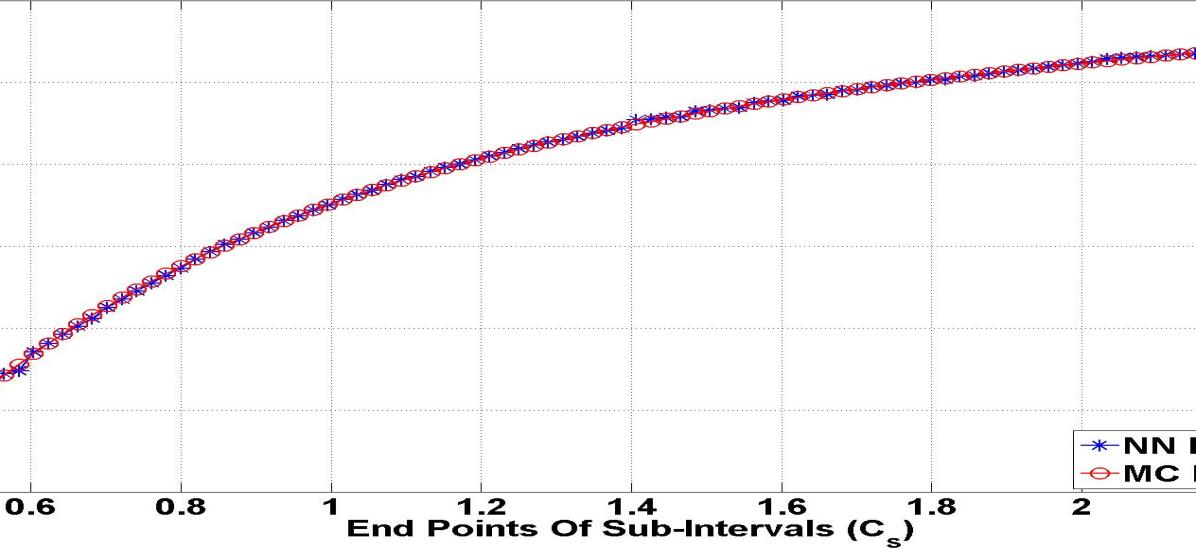
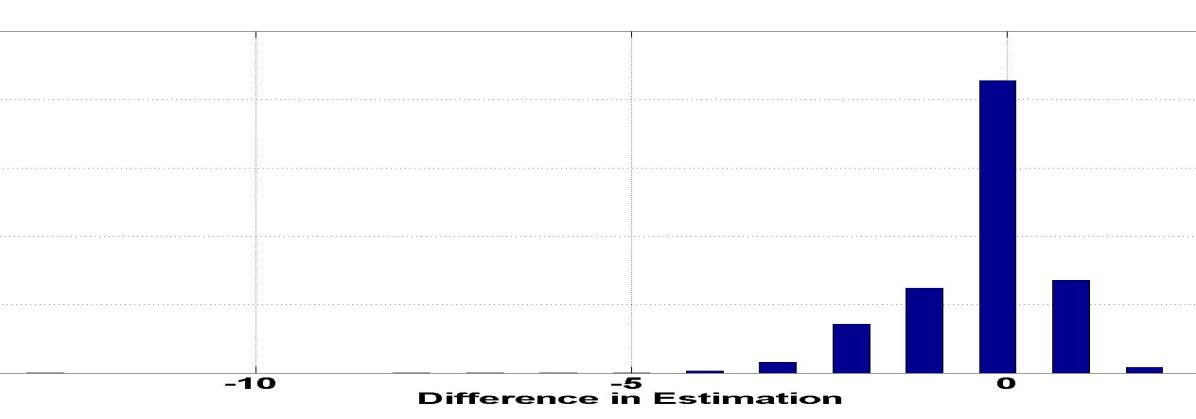
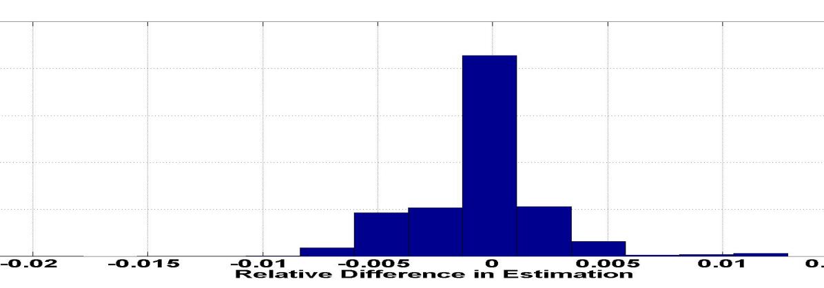
Table 5 presents the statistics on the running time of the proposed neural network approach for the nested simulation framework (denoted as NN in this table and elsewhere in the paper) and the nested MC simulation framework. The results suggest a speed-up of times, depending on the scenario, and an average speed-up of times. Considering that the implementation of the neural network was sequential and we compared the running time of the neural network with the implementation of MC simulations that uses parallel processing on 4 cores, we observe that even a simple implementation of the neural network can be highly efficient. As noted earlier, there is significant potential for parallelism in our neural network approach as well. Exploiting this parallelism should further improve the running time of the neural network. We plan to investigate this in a future paper. In addition, notice that we used a moderate number of MC simulation scenarios compared to the suggested values in (Bauer et al., 2012). As we mention earlier, an increase in the number of MC scenarios will not increase the running time of our neural network significantly, because we only need MC simulations for the representative contracts and for the validation/training portfolio; however, it increases the running time of the MC simulations significantly.
| Method | Running Time | |
|---|---|---|
| Mean | STD | |
| MC | ||
| NN | ||
6 Concluding Remarks
The new regulatory framework of Solvency II has been introduced by the European Union to reduce the risk facing insurance/re-insurance companies. An important part of the new regulations is the calculation of the SCR. Because of the imprecise language used to describe the standards, many insurance companies are struggling to understand and implement the framework.
In recent years, mathematical frameworks for calculation of the SCR have been proposed to address the former issue (Christiansen and Niemeyer, 2014; Bauer et al., 2012). Furthermore, (Bauer et al., 2012) has suggested a nested MC simulation approach to calculate the SCR to address the latter issue. The suggested MC approach is computationally expensive, even for one simple insurance contract. The computational complexity of the framework stems from two factors: 1) the large number of outer simulation scenarios, representing different market conditions, required to estimate the probability distribution of the and 2) the need to perform a computationally demanding MC simulation for each outer simulation scenario to calculate the value of the liability for the insurance policy under that scenario.
In this paper, we focus on the latter issue for a large portfolio of insurance products and propose a spatial interpolation approach to be used within the nested MC simulation framework for the liability calculation that uses a neural network engine to interpolate the liability values of insurance products based on the known liability values of a small representative set of these products. We study the performance of the proposed approach in finding the SCR value for a portfolio of VA products. The results of our numerical experiments in Section 5 corroborate the superior accuracy and efficiency of the sequential implementation of our proposed neural network approach compared with an implementation of the standard nested MC simulation approach that uses parallel processing to do the MC simulations.
Although our method requires us to train our neural network using three small ( of the input portfolio) portfolios that are selected uniformly at random, given an appropriate size for each of the small portfolios, the performance of the method has low sensitivity to the particular realization of these portfolios.
Despite the superior performance of the proposed approach that uses a simple uniform sampling method to select the small portfolios required to train the network, we believe our neural network approach can be further improved by incorporating a more sophisticated sampling method that takes into account the distribution of the input portfolio. We intend to address this issue in our future research.
The neural network that we used in our experiments was implemented sequentially. Given the structure of parameters/variables that define the behavior of the neural network, we can easily develop a parallel implementation of the neural network. A parallel implementation can significantly reduce the training time of the neural network and thereby the running time of the neural network framework. We plan to address this issue in our future work.
Although, in this paper, we do not study in depth the problem of having a large number of outer simulation scenarios, we proposed a possible solution via data interpolation to alleviate this problem. In our experiments, to reduce the simulation times and because of the smoothness of the curve that describes the values, as a first simple choice, we suggest using piecewise-linear interpolation to approximate the values. However, our experimental results suggest that using a better interpolation method can increase the accuracy of our proposed neural network approach for nested simulations. We intend to study the choice of the interpolation scheme in our future research.
In this introductory paper on our neural network approach, we chose to focus on a simple model of financial markets to make our analysis more tractable. However, as we discuss in Sections 3 and 5, the approach can be extended to incorporate more complex models of financial markets. To achieve the best outcome with our neural network approach, we need to study an effective strategy to exploit the closeness of the sample points representing various states of the financial markets to reduce the training time of the neural network. We intend to study this in our future work.
In this paper, we chose to study the performance of our neural network approach on estimation of liabilities; however, the application of our proposed approach is much more general than that. In particular, one can change the type of the insurance product and the approach used to value individual insurance products and incorporate them within our framework to estimate the value of a large portfolio of the aforementioned insurance products.
7 Acknowledgements
This research was supported in part by the Natural Sciences and Engineering Research Council of Canada (NSERC).
References
- CEIOP (2011) CEIOP, EIOPA Report on the Fifth Quantitative Impact Study (QIS5) for Solvency II URL https://eiopa.europa.eu/Publications/Reports/QIS5_Report_Final.pdf.
- Christiansen and Niemeyer (2014) M. C. Christiansen, A. Niemeyer, Fundamental Definition of the Solvency Capital Requirement in Solvency II, ASTIN Bulletin 44 (3) (2014) 501–533.
- Bauer et al. (2012) D. Bauer, A. Reuss, D. Singer, On the Calculation of the Solvency Capital Requirement Based on Nested Simulations, ASTIN Bulletin 42 (2012) 453–499, ISSN 1783–1350.
- TGA (2013) TGA, Variable Annuities—An Analysis of Financial Stability, The Geneva Association URL https://www.genevaassociation.org/media/ga2013/99582-variable-annuities.pdf.
- Hejazi et al. (2015) S. A. Hejazi, K. R. Jackson, G. Gan, A Spatial Interpolation Framework for Efficient Valuation of Large Portfolios of Variable Annuities, URL http://www.cs.toronto.edu/pub/reports/na/IME-Paper1.pdf, 2015.
- IRI (2011) IRI, The 2011 IRI Fact Book, Insured Retirement Institute .
- Girard (2002) L. Girard, An Approach to Fair Valuation of Insurance Liabilities Using the Firm’s Cost of Capital, North American Actuarial Journal 6 (2002) 18–41.
- Dembo and Rosen (1999) R. Dembo, D. Rosen, The Practice of Portfolio Replication: A Practical Overview of Forward and Inverse Problems, Annals of Operations Research 85 (1999) 267–284.
- Oechslin et al. (2007) J. Oechslin, O. Aubry, M. Aellig, A. Kappeli, D. Br̈onnimann, A. Tandonnet, G. Valois, Replicating Embedded Options in Life Insurance Policies, Life & Pensions (2007) 47–52.
- Daul and Vidal (2009) S. Daul, E. Vidal, Replication of Insurance Liabilities, RiskMetrics Journal 9 (1) (2009) 79–96.
- Cathcart and Morrison (2009) M. Cathcart, S. Morrison, Variable Annuity Economic Capital: the Least-Squares Monte Carlo Approach, Life & Pensions (2009) 36–40.
- Longstaff and Schwartz (2001) F. Longstaff, E. Schwartz, Valuing American Options by Simulation: A Simple Least-Squares Approach, The Review of Financial Studies 14 (1) (2001) 113–147.
- Carriere (1996) J. Carriere, Valuation of the Early-Exercise Price for Options Using Simulations and Nonparametric Regression, Insurance: Mathematics and Economics 19 (1) (1996) 19–30.
- Gan (2013) G. Gan, Application of Data Clustering and Machine Learning in Variable Annuity Valuation, Insurance: Mathematics and Economics 53 (3) (2013) 795–801.
- Gan and Lin (2015) G. Gan, X. S. Lin, Valuation of Large Variable Annuity Portfolios Under Nested Simulation: A Functional Data Approach, Insurance: Mathematics and Economics 62 (0) (2015) 138–150.
- Hejazi and Jackson (2016) S. A. Hejazi, K. R. Jackson, A Neural Network Approach to Efficient Valuation of Large Portfolios of Variable Annuities, Insurance: Mathematics and Economics 70 (2016) 169–181.
- Nadaraya (1964) E. A. Nadaraya, On Estimating Regression, Theory of Probability and its Applications 9 (1964) 141–142.
- Watson (1964) G. S. Watson, Smooth Regression Analysis, Sankhyā: Indian Journal of Statistics 26 (1964) 359–372.
- Hejazi (2016) S. A. Hejazi, A Neural Network Approach to Efficient Valuation of Large VA Portfolios, Ph.D. thesis, University of Toronto, In preparation, 2016.
- Bishop (2006) C. M. Bishop, Pattern Recognition and Machine Learning (Information Science and Statistics), Springer-Verlag, NJ, USA, 2006.
- Fister et al. (2016) I. Fister, P. N. Suganthan, S. M. Kamal, F. M. Al-Marzouki, M. Perc, D. Strnad, Artificial neural network regression as a local search heuristic for ensemble strategies in differential evolution, Nonlinear Dynamics 84 (2) (2016) 895–914.
- Boyd and Vandenberghe (2004) S. Boyd, L. Vandenberghe, Convex Optimization, Cambridge University Press, NY, USA, 2004.
- Murphy (2012) K. P. Murphy, Machine Learning: A Probabilistic Perspective, The MIT Press, 2012.
- Nesterov (1983) Y. Nesterov, A Method of Solving a Convex Programming Problem with Convergence Rate O(1/sqrt(k)), Soviet Mathematics Doklady 27 (2) (1983) 372–376.
- Sutskever et al. (2013) I. Sutskever, J. Martens, G. Dahl, G. Hinton, On the Importance of Initialization and Momentum in Deep Learning, in: Proceedings of the 30th International Conference on Machine Learning (ICML-13), vol. 28, JMLR Workshop and Conference Proceedings, 1139–1147, 2013.
- Hull (2006) J. C. Hull, Options, Futures, and Other Derivatives, Pearson Prentice Hall, Upper Saddle River, NJ, 6th edn., 2006.