PetroSurf3D – A Dataset for high-resolution 3D Surface Segmentation

Abstract

The development of powerful 3D scanning hardware and reconstruction algorithms has strongly promoted the generation of 3D surface reconstructions in different domains. An area of special interest for such 3D reconstructions is the cultural heritage domain, where surface reconstructions are generated to digitally preserve historical artifacts. While reconstruction quality nowadays is sufficient in many cases, the robust analysis (e.g. segmentation, matching, and classification) of reconstructed 3D data is still an open topic. In this paper, we target the automatic and interactive segmentation of high-resolution 3D surface reconstructions from the archaeological domain. To foster research in this field, we introduce a fully annotated and publicly available large-scale 3D surface dataset including high-resolution meshes, depth maps and point clouds as a novel benchmark dataset to the community. We provide baseline results for our existing random forest-based approach and for the first time investigate segmentation with convolutional neural networks (CNNs) on the data. Results show that both approaches have complementary strengths and weaknesses and that the provided dataset represents a challenge for future research.

I Introduction

Today, powerful techniques for the reconstruction of 3D surfaces exist, such as laser scanning, structure from motion and structured light scanning [1]. The result is an increased availability of surface reconstructions with high resolutions at sub-millimeter scale. At these high resolutions it is possible to capture the geometric fine structure (i.e. the topography [2]) of a surface. The surface topography determines the tactile appearance of a surface and is thus characteristic for different materials and differently rough surfaces. The automatic segmentation and classification of surfaces according to their topography is an essential pre-requisite for reliable large scale analyses, however, it is still an open problem.

A crucial requirement for the development of automatic surface segmentation algorithms are publicly available datasets with precise manual annotations (ground truth). A large number of datasets has been published for 2D and 3D texture analysis and material classification [3, 4, 5]. Usually, no geometric information is provided with these datasets i.e., the datasets contain only images of the surfaces (potentially with different lighting directions). Automatic segmentation methods, however, are supposed to benefit strongly from full 3D geometric information compared to only 2D (RGB) texture. Other datasets, employed for semantic segmentation, indeed provide 3D information [6, 7, 8, 9, 10, 11] but at a completely different spatial scale. These datasets are usually captured using off-the-shelf depth cameras (e.g. Microsoft Kinect) and have primarily been developed for scene understanding and object recognition. Thus, they show entire objects and scenes and provide resolutions at centimeter level. These datasets address a different task and are too coarse to capture the characteristics of different types of surfaces and materials.

In this paper, we present a dataset of high-resolution 3D surface reconstructions which contains full geometry information as well as color information and thus resembles both the tactile and visual appearance of the surfaces at a micro scale. The surfaces stem from the archaeological domain and represent natural rock surfaces into which petroglyphs (i.e. symbols, figures and abstractions of objects) have been pecked, scratched or carved in ancient times. The engraved motifs represent areas with different roughness and tactile structure and exhibit complex and heterogeneous shapes. Hundreds or in most cases even thousands of years of weathering and erosion rendered many petroglyphs indistinguishable from the natural rock surface with the naked eye or by using 2D imagery. These properties make the scanned surfaces a challenging testbed for the evaluation of automatic 2D and 3D surface segmentation algorithms.

This paper builds upon a series of incremental previous works on 3D surface segmentation and classification [12, 13, 14] and intends to consolidate and extend the achieved results. Our contribution beyond previous research are as follows:

• We present a novel benchmark dataset for surface segmentation of high-resolution 3D surfaces to the public that enables objective comparison between novel surface segmentation techniques.

• We provide precise ground truth annotations generated by experts from archeology for the evaluation of surface segmentation algorithms together with a reproducible evaluation protocol.

• We provide baselines for our existing approach [13, 14] and a novel CNN-based approach to enable instant performance comparisons.

• We comprehensively evaluate the generalization ability of the proposed approaches and the benefit of using full 3D information for segmentation compared to pure 2D texture segmentation.

II Dataset

Our fully labeled 3D dataset of rock surfaces with petroglyphs is publicly available. In a large effort, we scanned petroglyphs on several different rocks at sub-millimeter accuracy. From the 3D scans we created meshes and point clouds and additionally orthophotos and corresponding depth maps to enable the application of 3D and 2D segmentation approaches on the data. Note that, since there are usually no self-occlusions in pecked rock surfaces, the 3D information is almost fully preserved in the depth maps (except for rasterization artifacts). For all depth maps and orthophotos we provide pixel-wise ground truth labels (overall about 232 million labeled pixels) and the parameters for the mapping from 3D space to 2D (and vice versa).

II-A Dataset Acquisition

The surface data has been acquired at the UNESCO World heritage site in Valcamonica, Italy, which provides one of the largest collections of rock art in the world. The data has been scanned by experts using two different scanning techniques: (i) structured light scanning (SLS) with the Polymetric PTM1280 scanner in combination with the associated software QTSculptor and (ii) structure from motion (SfM). For SfM, photos were acquired with a high-quality Nikkor 60 mm macro lense mounted on a Nikon D800. For bundle adjustment the SfM engine of the software package Aspect3D was used and SURE was employed for the densification of the point clouds. The point clouds have been denoised by removing outliers which stand out significantly from the surface [15] and smoothed by a moving least squares filter. The resulting point clouds have a sampling distance of at least 0.1 mm and provide RGB color information for each 3D vertex. The vertex coordinates are in metric units relative to a base station. We provide the point clouds in XYZRGB format. Additionally, the point clouds were meshed by Poisson triangulation. Meshes were textured with the captured vertex colors and are provided in WRL format.

We generated orthophotos and depth maps of all surface reconstructions. For the rasterization of the projected images we used a resolution of 300dpi (i.e., 0.08 mm pixel side length). The ortho projections were derived from the meshed 3D data since this enables a dense projection without holes. The depth maps are stored as 32-bit TIFF files.

For each surface a pixel-accurate ground truth has been generated by archaeologists who labeled all pecked regions on the surface. Since the surfaces contain no self-occlusions the annotators worked directly on the 2D orthophotos and depth maps. The annotators spent several hours on each surface depending on the size and complexity of the depicted engraving, e.g. anthropomorph, inscription, symbol, etc. Anthropogenically altered, i.e. pecked, areas were annotated with white color, whereas the natural rock surface remained black and regions outside the scan were colored red. The provided geometric mapping information between the 3D point cloud and the ortho projections allows to easily map the ground truth to the point cloud and the mesh for processing in the 3D space.

II-B Dataset Overview

The final dataset contains 26 high-resolution surface reconstructions of natural rock surfaces with a large number of petroglyphs. Tab. I provides some basic measures for each reconstruction, such as number of points, covered area, percentage of pecked surface area etc. The petroglyphs have been captured at various locations at three different sites in the valley: “Foppe di Nadro” (IDs 1-3), “Naquane” (IDs 4-10), and “Seradina” (IDs 11-26). The point clouds of all surfaces together sum up to overall 115 million points. They cover in total an area of around 1.6 m². After projection to orthophotos and depth images this area corresponds to around 232 million pixels. Note that there are more pixels than 3D points due to the interpolation that takes place during projection of the mesh.

TABLE I: Overview of basic measures of the digitized surfaces: the covered area (in pixels at 300dpi and in cm²), the number of 3D points in the point cloud, the percentage of pecked regions, the number of disconnected pecked regions, the range of depth values

ID	Covered Area		Num.	Percentage	Num.	Depth Range
	in px	in cm2	3D Pts.	Pecked	Seg.	in mm
1	5 143 296	368.69	3 264 005	$14.61$	$48$	$2.89$
2	15 638 394	1121.03	10 280 976	$10.56$	$21$	$4.83$
3	8 846 214	634.14	5 503 742	$47.63$	$18$	$9.11$
4	15 507 622	1 111.66	3 782 381	$14.96$	$17$	$62.52$
5	16 994 561	1 218.25	2 658 330	$17.27$	$44$	$70.60$
6	13 102 254	939.23	1 260 401	$12.67$	$13$	$49.32$
7	12 035 386	862.75	810 312	$34.02$	$26$	$15.17$
8	12 834 446	920.03	8 677 163	$26.17$	$45$	$6.74$
9	12 835 586	920.11	8 386 259	$32.83$	$29$	$3.82$
10	5 901 454	423.04	2 096 476	$21.59$	$9$	$5.41$
11	5 632 144	403.74	3 541 799	$9.26$	$23$	$10.23$
12	7 103 936	509.24	4 432 013	$5.09$	$6$	$10.22$
13	6 155 628	441.26	3 810 000	$8.26$	$63$	$19.85$
14	5 855 280	419.73	4 417 779	$6.47$	$17$	$10.50$
15	4 855 764	348.08	2 981 570	$4.44$	$24$	$9.39$
16	4 029 231	288.83	2 523 543	$6.58$	$29$	$4.27$
17	4 838 487	346.84	3 022 433	$3.15$	$27$	$21.75$
18	6 396 152	458.50	4 007 232	$19.41$	$25$	$9.45$
19	7 141 253	511.92	4 472 845	$18.20$	$32$	$17.32$
20	6 864 476	492.08	4 238 990	$12.02$	$15$	$21.39$
21	3 909 579	280.26	2 255 030	$20.40$	$61$	$5.32$
22	4 073 804	292.03	2 395 125	$16.34$	$65$	$3.99$
23	3 612 131	258.93	2 113 670	$24.23$	$54$	$5.33$
24	19 104 798	1 369.52	10 685 564	$26.61$	$152$	$27.35$
25	14 920 005	1 069.53	8 188 025	$15.55$	$63$	$17.49$
26	8 921 684	639.55	5 515 973	$15.59$	$99$	$16.62$
Overall	232 253 565	16 648.97	115 321 636	$18.68$	$1025$	[2.89, 70.60]

The scans show isolated figures as well as scenes with multiple interacting petroglyphs (e.g. hunting scenes). The pecked regions in all reconstructions are disconnected and in average consist of about 40 segments. The pecked regions make up around 19% of the entire scanned area.

An example surface of the dataset is shown in Fig. 1. We depict the orthophoto, the corresponding depth map and the ground truth labels. Note that the peckings are sometimes virtually unrecognizable from the orthophoto and can hardly be discovered without taking the ground truth labels into account. Further note the strong variation in depth ranges which stems from the shape and curvature of the rock surfaces themselves.

(a)

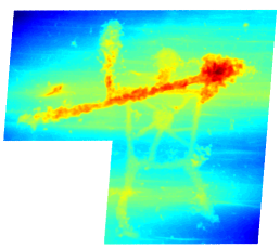
(b)

(c)

Figure 1: Example orthophoto (left), corresponding depth map (center), and ground truth labels (right). For visualization of the depth, we normalized and cropped the distance ranges per scan and show the resulting values in false color. Best viewed in color on screen with zoom

III Experiments

In this section we present baseline experiments for our dataset. We have published some complementary results on the dataset previously [13] where we focused on interactive segmentation and different types of hand-crafted surface features. In contrast to our previous work, in this paper we focus on fully automatic segmentation and learned features. Aside from providing an evaluation protocol and baselines of state-of-the-art approaches we investigate the following questions related to our dataset in detail: (i) What is the benefit of using 3D depth information compared to pure texture information (RGB) for surface segmentation of petroglyphs? (ii) Can our learned models generalize from rock surfaces of one location to surfaces of another location (generalization ability)?

III-A Evaluation Protocol

To enable reproducible and comparable experiments, we propose the following two evaluation protocols on the dataset:

4-fold Cross-Validaion: To obtain results for the whole dataset, we perform a $k$-fold cross-validation, with the number of folds being $k=4$. We randomly assigned the surface reconstructions to the folds. The assignment of surfaces to folds is provided with the dataset.

Cross-Site Generalization: Here we separate the dataset into two sets according to the geographical locations the scans were captured at. We employ one of the two sets as training set and the other one as test set, and vice-versa. In this way, we obtain insights about the generalization ability of a given approach across data from different capture locations.

The latter protocol is especially interesting since, on the one hand, the rock surfaces vary between sites, and on the other hand, the petroglyphs at different sites exhibit different shapes and peck styles, e.g., due to different tools that were used for their creation. We separate the dataset into one set containing the scans from Seradina and the other one containing the scans from Foppe di Nadro and Naquane. Foppe di Nadro and Naquane were joined because these sites are situated next to each other and the corresponding petroglyphs are rather similar. For evaluation we use one of the two sets as training set and the other one as test set, and vice-versa. This results in the following three experiments:

• Training on data from Foppe di Nadro and Naquane; testing on Seradina.

• Training on data from Seradina; testing on Foppe di Nadro.

• Training on data from Seradina; testing on Naquane.

In this way each surface reconstruction is exactly once in the test set.

Metrics

For quantitative evaluations on our dataset we propose a number of metrics commonly used for semantic segmentation to enable reproducible experiments. In our case the segmentation task is a pixelwise binary problem and, hence, the evaluation is based on the predicted segmentation mask and the ground truth mask. Based on these masks we compute the Jaccard index [16], also often termed region based intersection over union ($IU$), for which we compute the average over classes ($mIU$) as in [17, 18, 19, 20], the pixel accuracy (PA) [21, 20], the dice similarity coefficient ($DSC$) [14], the hit rate ($HR$) [20, 14] and the false acceptance rate ($FAR$) [14].

III-B Methods

To provide a baseline we evaluate the performance of prominent state-of-the-art approaches for semantic segmentation on our dataset. First, we perform experiments with a segmentation method based on Random Forests (RF). Second, we apply Convolutional Neural Networks (CNNs) [22, 23], which currently show best performance on standard semantic segmentation benchmarks [17, 18, 19, 24, 25] and compare them with the RF-based approach. We have shown previously that surface segmentation with 3D descriptors computed directly from the 3D point clouds is computationally demanding and with current state-of-the-art methods not performing well, see [12] for respective results for a subset of our dataset. Hence, we employ the depth maps and orthophotos generated from the point clouds as input to segmentation.

For Random Forests (RFs) we employed an approach, which was also used as a baseline in many other RF-based works on semantic segmentation [26, 27, 28]. That is, we trained a classification forest [29] to compute a pixelwise labeling of the scans. The Random Forest is trained on patches representing the spatial neighborhood of the corresponding pixel. To this end, we downscaled the scans by a factor of five and extracted patches of size $17\times 17$ corresponding to a side length of 6.8 mm. We randomly sampled 8000 patches – balanced over the classes – from each training image. As features we used the color or depth values directly. For all experiments we trained 10 trees, for which we stopped training when a maximum depth of 18 was reached or less than a minimum number of 5 samples arrived in a node.

In the CNN-based approach we employ fully convolutional neural networks as proposed in [17], since this work has been very influential for several following CNN-based methods for semantic segmentation [24, 19, 25]. To perform petroglyph segmentation on our dataset we finetune a model, which was pre-trained for semantic segmentation on the PASCAL-Context dataset [30]. To create training data for finetuning we again downscaled the depth maps by a factor of 5 and randomly sampled $224\times 224$ pixel crops. To generate enough training data for finetuning the CNN and additionally increase the variation in the training set, we augment it with randomly rotated versions of the depth maps ($r\in\{0,45,90,\ldots,315\}$ degrees) prior to sampling patches. Similarly, we flip the depth-maps with a probability of 0.5. Note, that rotating the images randomly is reasonable since the petroglyphs have no unique orientation on the rock surfaces. Using the described augmentation strategy we sampled about 5000 crops, while ensuring that each crop contains pixel labels from both classes. We finetuned for a maximum of 30 epochs. For finetuning we employ Caffe [31] and set the learning rate to $5\times 10^{-9}$. Due to GPU memory limitations (3GB) we were only able to use a batch size of one (i.e. one depth map at a time). We, thus, follow [21] and use a high momentum of $0.98$, which approximates a higher batch size and might also yield better accuracy due to the more frequent weight updates [21].

III-C 2D vs. 3D Segmentation

In a first experiment we investigate the importance of 3D information provided by our dataset compared to pure color-based surface segmentation. Therefore, we train a Random Forest (RF) only with color information from the orthophotos and compare the results to a RF trained on only depth information. For this experiment we follow the 4-fold cross-validation protocol specified in Sec. III-A. The results in Tab. II (rows 1 and 2) clearly show the necessity for 3D information to obtain good results. This is further underlined in Fig. 2, where the results are compared for each individual scan. We observe that depth information improves results nearly for each scan by a large margin. This can be explained by the fact that engraved surface regions often resemble the visual appearance of the surrounding rock surface due to influences from weathering.

TABLE II: Quantitative results for different setups, comparing the capabilities of color (2D) and depth (3D) information. 3D segmentation strongly outperforms color-based 2D segmentation

Representation	HR	FAR	DSC	mIU	PA
Color	0.493	0.675	0.392	0.465	0.715
Depth	0.779	0.553	0.568	0.569	0.779
Depth – Cross-Sites	0.777	0.574	0.550	0.551	0.763

Note that we also experimented with combining color and depth information, as well as with different features like image gradients, LBP features [32], and Haralick features [33] to abstract the pure color and depth information. However, these had little to no impact on the final segmentation performance and, hence, the results are omitted for brevity.

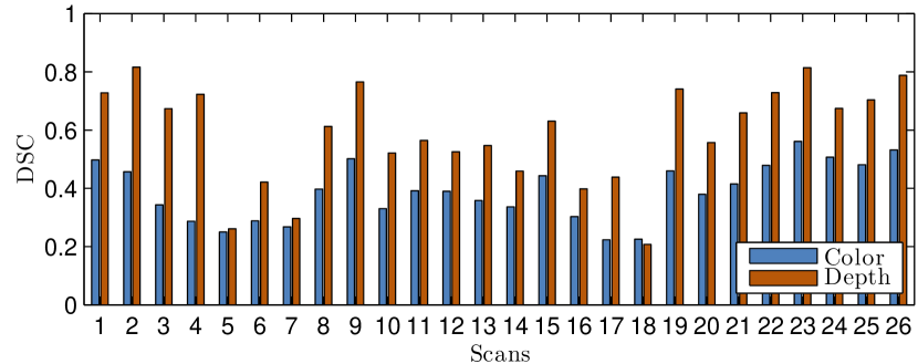
Figure 2: Dice Similarity Coefficient ($DSC$) per scan

III-D Baseline Results

In this section we present the results of the baseline methods for the two proposed evaluation protocols.

III-D1 Cross-Site Generalization

The results for Random Forests for the proposed cross-site evaluation protocol (see Sec. III-A) are listed in Tab. III. Here, we provide the detailed results for each of the three splits. Overall results averaged over all three experiments are shown in Tab. II (last row) for comparison with the experiments in Sec. III-C. Interestingly, the overall results are in the same range as the results of the 4-fold cross-validation with randomly selected folds. This suggests that – using 3D information – an automatic method is able to generalize from one site of the valley to another.

TABLE III: Results for cross-validation over different sites. Quantitative results obtained for scans from Seradina when an RF classifier is trained on scans of only Foppe di Nadro and Naquane, as well as results for scans from Foppe di Nadro and Naquane when the classifier is trained only on scans of Seradina

Training Set:	Foppe di Nadro $+$ Naquane	Seradina	Seradina
Test Set:	Seradina	Foppe di Nadro	Naquane
HR	0.843	0.706	0.744
FAR	0.544	0.274	0.644
DSC	0.592	0.716	0.482
mIU	0.612	0.704	0.446
PA	0.827	0.875	0.645

III-D2 4-fold Cross-Validation

To provide a more comprehensive baseline for the performance of state-of-the-art methods we compare the results obtained with Random Forests (RFs) and Convolutional Neural Networks (CNNs) both evaluated on depth information. For the CNN, which was pre-trained on color images (see Section III-B) we simply fill all three input channels with the same depth channel to obtain a compatible input format. Additionally, we subtract the local average depth value from each pixel in the depth map to normalize the input data, which was necessary to stay compatible to the CNN pre-trained on RGB data. This normalization can be efficiently performed in a pre-processing step by subtracting a smoothed version of the depth map (Gaussian filter with $\sigma=12.5\,\mathrm{mm}$) from the depth map. This operation results in a local constrast equalization across the depth map [12] that better enhances the fine geometric details of the surface texture.

Quantitative results for the whole dataset are shown in Tab. IV. The quantitative results in terms of mIU for each surface are visualized in Fig. 3. In Fig. 4 we show some qualitative results for each method. From the results we observe that the Random Forest (RF) yields more cluttered results, whereas the the CNN yields more consistent but coarser segmentations. The RF correctly detects small and thin pecked regions, which the CNN misses, whereas the CNN usually captures the overall shape of the petroglyphs more accurately but misses details. Note that for none of the results we applied Conditional or Markov Random Fields (MRFs, CRFs) or similar models, since we want to enable easier comparisons to our baselines. We assume that the reasons for the differences of RF and CNN are (i) that the RF makes independent pixel-wise decisions whereas the CNN implicitly considers the spatial context through its learned feature hierarchy and (ii) that the receptive field of the RF is smaller than the receptive field of the CNN. This is because the CNN is able to exploit additional spatial information through its hierarchy of filters while the RF was unable to effectively exploit larger receptive fields in our experiments.

The complementary abilities of RF and CNN are further reflected in the quantitative results in Tab. IV. The more consistent and coarser segmentations of the CNN yield a better overall segmentation result which is reflected by the higher DSC, mIU, and PA values. For the foreground class in particular the HR of RF outperforms that of CNN which means that a higher percentage of foreground pixels is labeled correctly. The reason for this is that CNN often misses larger portions of the pecked regions.

TABLE IV: 4-fold cross-validation results for Random Forests (RFs) and Convolutional Neural Networks (CNNs)

Method	HR	FAR	DSC	mIU	PA
RF	0.779	0.553	0.568	0.569	0.779
CNN	0.693	0.357	0.667	0.676	0.871

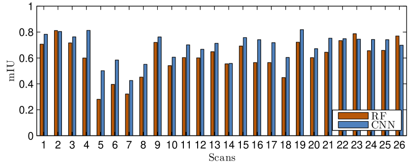
Figure 3: Mean intersection over union ($mIU$) per scan

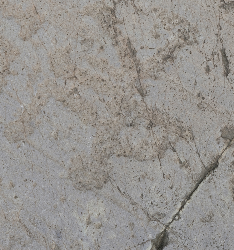
(a) RGB

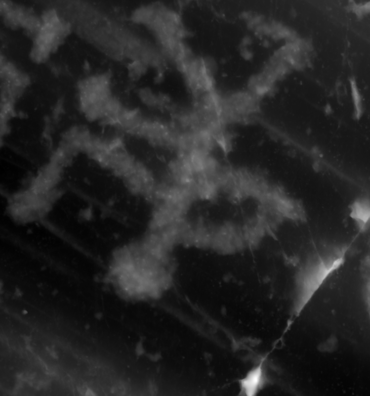
(b) Depth map

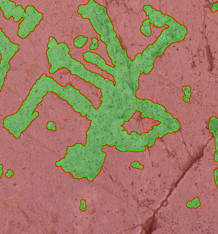
(c) Ground truth

(d) RF result

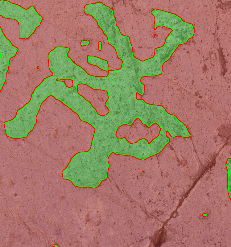
(e) CNN result

(f) RGB

(g) Depth map

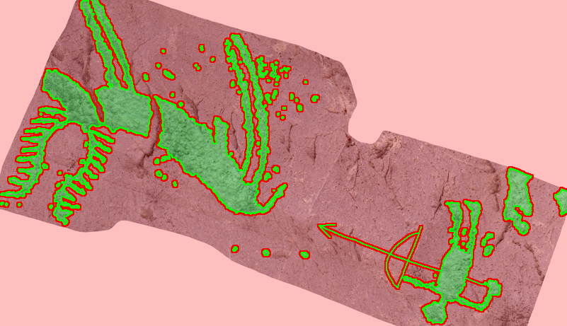
(h) Ground truth

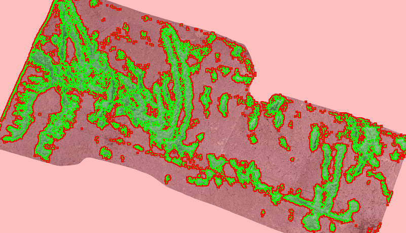
(i) RF result

(j) CNN result

Figure 4: Input images (orthophotos and depth maps), ground truth labelings and results for the CNN and the RF baselines. Best viewed on screen with zoom.

IV Conclusions

In this paper, we introduced a novel dataset for 3D surface segmentation. The dataset contains reconstructions of natural rock surfaces with complex-shaped engravings (petroglyphs). The main motivation for contributing the dataset to the community is to foster, in general, research on the automated semantic segmentation of 3D surfaces and, in particular, the segmentation of petroglyphs as a contribution to the conservation of our cultural heritage. We complement the dataset with accurate expert-annotated ground-truth, an evaluation protocol and provide baseline results for two state-of-the-art segmentation methods.

Our experiments show that (i) depth information – as provided by our dataset – is imperative for the generalization ability of segmentation methods and pure 2D segmentation is insufficient for this dataset; (ii) in most cases, the use of CNN classification outperforms RFs in terms of quantitative measures and, qualitatively, the CNN yields rougher but more consistent segmentations than RFs. The obtained results (baseline DSC of 0.667) show that the dataset is far from being solved and thus represents a challenge for 3D surface segmentation in future.

References

- [1] C. Wu, “Towards linear-time incremental structure from motion,” in 3D Vision - 3DV 2013, 2013 International Conference on, June 2013, pp. 127–134.
- [2] L. Blunt and X. Jiang, Advanced techniques for assessment surface topography: development of a basis for 3D surface texture standards “surfstand”. Elsevier, 2003.
- [3] K. J. Dana, B. van Ginneken, S. K. Nayar, and J. J. Koenderink, “Reflectance and texture of real-world surfaces,” ACM Trans. on Graphics, vol. 18, no. 1, pp. 1–34, 1999.
- [4] T. Ojala, T. Mäenpää, M. Pietikäinen, J. Viertola, J. Kyllönen, and S. Huovinen, “Outex- new framework for empirical evaluation of texture analysis algorithms,” in Proc. Int’l Conf. on Pattern Recognition, 2002.
- [5] M. Haindl and S. Mikeš, “Texture segmentation benchmark,” in Proc. Int’l Conf. on Pattern Recognition, 2008.
- [6] M. Firman, “RGBD datasets: Past, present and future,” in CVPR Workshop on Large Scale 3D Data: Acquisition, Modelling and Analysis, 2016.
- [7] I. Armeni, A. Sax, A. R. Zamir, and S. Savarese, “Joint 2D-3D-semantic data for indoor scene understanding,” arXiv preprint arXiv:1702.01105, 2017.
- [8] S. Song, S. P. Lichtenberg, and J. Xiao, “SUN RGB-D: A RGB-D scene understanding benchmark suite,” in Proc. IEEE Conf. on Computer Vision and Pattern Recognition, 2015.
- [9] P. K. Nathan Silberman, Derek Hoiem and R. Fergus, “Indoor segmentation and support inference from RGBD images,” in Proc. European Conf. on Computer Vision, 2012.
- [10] A. Janoch, S. Karayev, Y. Jia, J. T. Barron, M. Fritz, K. Saenko, and T. Darrell, “A category-level 3-d object dataset: Putting the kinect to work,” in ICCV Workshop on Consumer Depth Cameras for Computer Vision, 2011.
- [11] N. Silberman and R. Fergus, “Indoor scene segmentation using a structured light sensor,” in ICCV Workshop on 3D Representation and Recognition, 2011.
- [12] M. Zeppelzauer and M. Seidl, “Efficient image-space extraction and representation of 3d surface topography,” in Proc. Int’l Conf. on Image Processing, 2015.
- [13] M. Zeppelzauer, G. Poier, M. Seidl, C. Reinbacher, C. Breiteneder, H. Bischof, and S. Schulter, “Interactive segmentation of rock-art in high-resolution 3d reconstructions,” in Proc. Int’l Conf. on Digital Heritage, 2015.
- [14] M. Zeppelzauer, G. Poier, M. Seidl, C. Reinbacher, S. Schulter, C. Breiteneder, and H. Bischof, “Interactive 3d segmentation of rock-art by enhanced depth maps and gradient preserving regularization,” Journal on Computing and Cultural Heritage (JOCCH), vol. 9, no. 4, p. 19, 2016.
- [15] R. B. Rusu, Z. C. Marton, N. Blodow, M. Dolha, and M. Beetz, “Towards 3d point cloud based object maps for household environments,” Robotics and Autonomous Systems, vol. 56, no. 11, pp. 927–941, 2008.
- [16] P. Jaccard, “The distribution of the flora in the alpine zone,” New Phytologist, vol. 11, no. 2, pp. 37–50, 1912.
- [17] J. Long, E. Shelhamer, and T. Darrell, “Fully convolutional networks for semantic segmentation,” in Proc. IEEE Conf. on Computer Vision and Pattern Recognition, 2015.
- [18] B. Hariharan, P. A. Arbeláez, R. B. Girshick, and J. Malik, “Hypercolumns for object segmentation and fine-grained localization,” in Proc. IEEE Conf. on Computer Vision and Pattern Recognition, 2015.
- [19] S. Zheng, S. Jayasumana, B. Romera-Paredes, V. Vineet, Z. Su, D. Du, C. Huang, and P. Torr, “Conditional random fields as recurrent neural networks,” in Proc. IEEE Int’l Conf. on Computer Vision, 2015.
- [20] P. Kontschieder, S. R. Bulò, M. Pelillo, and H. Bischof, “Structured labels in random forests for semantic labelling and object detection,” IEEE Trans. on Pattern Analysis and Machine Intelligence, vol. 36, no. 10, pp. 2104–2116, 2014.
- [21] E. Shelhamer, J. Long, and T. Darrell, “Fully convolutional networks for semantic segmentation,” IEEE Trans. on Pattern Analysis and Machine Intelligence, vol. PP, no. 99, pp. 1–12, 2016.
- [22] Y. LeCun, L. Bottou, Y. Bengio, and P. Haffner, “Gradient-based learning applied to document recognition,” Proceedings of the IEEE, vol. 86, no. 11, pp. 2278–2324, 1998.
- [23] A. Krizhevsky, I. Sutskever, and G. E. Hinton, “Imagenet classification with deep convolutional neural networks,” in Advances in Neural Information Processing Systems, 2012.
- [24] L. Chen, G. Papandreou, I. Kokkinos, K. Murphy, and A. L. Yuille, “Semantic image segmentation with deep convolutional nets and fully connected crfs,” in Proc. Int’l Conf. on Learning Representations, 2015.
- [25] G. Lin, C. Shen, A. van dan Hengel, and I. Reid, “Efficient piecewise training of deep structured models for semantic segmentation,” in Proc. IEEE Conf. on Computer Vision and Pattern Recognition, 2016.
- [26] D. Laptev and J. M. Buhmann, “Convolutional decision trees for feature learning and segmentation,” in Proc. German Conf. on Pattern Recognition, 2014.
- [27] P. Kontschieder, P. Kohli, J. Shotton, and A. Criminisi, “Geof: Geodesic forests for learning coupled predictors,” in Proc. IEEE Conf. on Computer Vision and Pattern Recognition, 2013.
- [28] S. R. Bulò and P. Kontschieder, “Neural decision forests for semantic image labelling,” in Proc. IEEE Conf. on Computer Vision and Pattern Recognition, 2014.
- [29] L. Breiman, “Random forests,” Machine Learning, vol. 45, no. 1, pp. 5–32, 2001.
- [30] R. Mottaghi, X. Chen, X. Liu, N. Cho, S. Lee, S. Fidler, R. Urtasun, and A. L. Yuille, “The role of context for object detection and semantic segmentation in the wild,” in Proc. IEEE Conf. on Computer Vision and Pattern Recognition, 2014.
- [31] Y. Jia, E. Shelhamer, J. Donahue, S. Karayev, J. Long, R. Girshick, S. Guadarrama, and T. Darrell, “Caffe: Convolutional architecture for fast feature embedding,” arXiv preprint arXiv:1408.5093, 2014.
- [32] T. Ojala and M. Pietikäinen, “Unsupervised texture segmentation using feature distributions,” Pattern Recognition, vol. 32, no. 3, pp. 477–486, 1999.
- [33] R. M. Haralick, K. S. Shanmugam, and I. Dinstein, “Textural features for image classification,” IEEE Trans. Systems, Man, and Cybernetics, vol. 3, no. 6, pp. 610–621, 1973.