Calculation of Stark resonance parameters for valence orbitals of the water molecule.

Abstract

An exterior complex scaling technique is applied to compute Stark resonance parameters for two molecular orbitals ($1b_{1}$ and $1b_{2}$) represented in the field-free limit in a single-center expansion. For electric DC field configurations that guarantee azimuthal symmetry of the solution the calculation is carried out by solving a two-dimensional partial differential equation in spherical polar coordinates using a finite-element method. The resonance positions and widths as a function of electric field strengths are shown for field strengths starting in the tunnelling ionization regime, and extending well into the over-barrier ionization region.

I Introduction

The study of water molecule vapour in strong fields has been an area of recent interest, particularly in the field of intermediate-energy ion-molecule collisions Murakami et al. (2012a, b); Luna et al. (2016); Gulyás et al. (2016); Hong et al. (2016); Errea et al. (2013); Nandi et al. (2013), where capture and direct ionization processes compete. Most of the theoretical studies are in the context of an independent-electron approximation which involves a molecular orbital (MO) representation. First studies of the properties of molecular orbitals exposed to laser pulses have also been performed Farrell et al. (2011); Falge et al. (2010).

For the problem of strong electric DC fields numerous investigations have been carried out for the hydrogen molecular ion, where interesting structures occur in the resonance width as a function of internuclear separation Tsogbayar and Horbatsch (2013a); Chu and Chu (2000); Plummer and McCann (1996). This also carries over to the case of low-frequency AC fields, i.e., infrared laser fields with the help of the Floquet method Tsogbayar and Horbatsch (2013b). Experimentally, the investigation of water vapour is challenging, but possible Werner et al. (1995); Gobet et al. (2001, 2004); Luna et al. (2007). Due to the importance of the water molecule in applied fields (e.g., radiation therapy) one should expect more work to be carried out in this research area in the near future.

From the point of view of a theoretical description, the subject is challenging due to the multi-center nature of the combined Coulomb interactions. Thus, many investigations in the context of electron/positron or ion scattering are carried out in single-center approximations for the molecular target. For a number of situations this approach appears to be successful in that ionization (and capture) cross sections are obtained which agree reasonably with experiment. This is in part the case since experiments are usually not sensitive to the orientation of the molecule during the collision.

A satisfactory description of the molecular structure of H₂O was obtained within the independent-electron approximation by the self-consistent field (SCF), or variational Hartree-Fock method with multi-center Slater orbitals Aung et al. (1968). The direct application of these orbitals for collisional or strong-field studies does represent significant computational and methodological challenges. An application of the SCF method using a single-center Slater basis has been available Moccia (1964a, b, c), and has been used in some collision studies Montanari and Miraglia (2014). The molecular orbitals for water from Moccia (1964c) have been compared to experimental electron spectroscopy studies Hafied et al. (2007), and also to more sophisticated calculations, and were found to give reasonable agreement with observations. For further studies of state-of-the art spectrocopy and calculations we refer the reader to Ning et al. (2008).

In order to use a variational SCF solution for collisional or strong-field perturbation studies one faces the need to define a consistent molecular Hamiltonian. In the present work we limit ourselves to two of the three molecular valence orbitals of the water molecule where the wave functions are dominated by a single angular momentum symmetry ($1b_{1}\approx 2p_{x}$ or $1b_{2}\approx 2p_{y}$); here we assume that the protons are in the $y-z$ plane, as shown in Fig. 1. For our approximate treatment it is straightforward to obtain an effective single-electron potential for each orbital. The calculation of Stark resonance parameters for these approximate single-center molecular orbitals does represent a first step to be followed by more ambitious modelling to be carried out in the future.

We present a complex scaling approach to study the effect of an external DC field on the $1b_{1}\approx 2p_{x}$ and $1b_{2}\approx 2p_{y}$ MO’s of H₂O, where the problem is expressed as a system of coupled partial differential equations (PDEs) with an effective potential that reflects the binding properties of each orbital. The paper is organized as follows: The problem as formulated in spherical polar coordinates is introduced in Sec. II, with some technical details concerning the construction of the electronic potential being described in Sec. II.1. The exterior complex scaling formalism and the implementation are explained in Sec. II.3. The numerical results are presented in Sec. III, followed by conclusions in Sec. IV. Atomic units ($\hbar=m_{e}=e=4\pi\epsilon_{0}=1$) are used throughout.

II PDE approach to the problem in spherical polar coordinates

The set of single-center wave functions introduced by Moccia Moccia (1964a, b, c) is taken as a starting point in the present approach. The general expression for the basis functions is defined by a Slater-type orbital Moccia (1964a)

$$f_{n,l,m}(\zeta,r,\theta,\phi) = \sqrt{\frac{(2\zeta)^{2n+1}}{(2n)!}}r^{n-1}\exp(-\zeta r)S_{l,m}(\theta,\phi),$$ (1)

where the angular part $S_{l,m}(\theta,\phi)$ represents real spherical harmonics. The expansion coefficients and non-linear coefficients $\{\zeta_{i}\}$, determined by Roothaan’s self-consistent-field procedure Roothaan (1951); Moccia (1964c), were used to construct a reduced form of the radial functions that describe all the molecular orbitals, and in particular the $1b_{1}$ and $1b_{2}$ states. In Fig. 2 we depict schematically how the orbitals are approximated as $|m|=1$ eigenstates of spherically symmetric potentials. For the purpose of this study, the expansion of the orbital functions was truncated at $n=2$ with their associated $(n,l,m)$ combinations.

The framework for the present study involves the construction of the electronic potential as an effective orbital-dependent potential $V_{\rm{eff}}(r)$ extracted from the single-center Moccia wave functions. Then we apply exterior complex scaling (ECS) to determine the numerical solution of the problem associated with a molecular orbital in the presence of a strong electric DC field applied along the $z-$direction. A partial differential equation (PDE) needs to be solved to determine the resonance position and width.

The Schrödinger equation for the bound-state problem is expressed in spherical polar coordinates as

$$[-\frac{1}{2}\frac{d^{2}}{dr^{2}}+\frac{\hat{L}^{2}}{2r^{2}}+V_{\rm{eff}}(r)]\psi = E\psi,$$ (2)

where $\hat{L}^{2}$ is the orbital angular momentum operator.

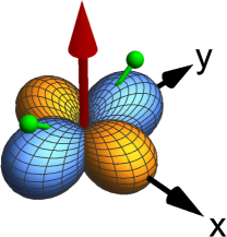
Figure 1: Schematic display of the $1b_{1}\approx 2p_{x}$ (shown in yellow) and $1b_{2}\approx 2p_{y}$ (shown in blue) molecular orbitals. Also indicated (in green) is the orientation of the protons. The $z$-axis (in red) is the direction of the external electric field of strength $F_{0}$.

Figure 1 shows a scheme of the geometry of the system, where the orientation of the $1b_{1}$ and $1b_{2}$ MO’s is represented with respect to the plane where the protons are located. The direction of the applied electric field along $\hat{z}$ is included as well.

II.1 Construction of an electronic effective potential

The effective potential is obtained in two steps: first the orbital energy and the STO are inserted into the single-electron Schrödinger equation (2) which is then solved for $V_{\rm{eff}}^{(1)}(r)$. In the second step we apply the so-called Latter correction Latter (1955) to ensure that the asymptotic behavior of the potential is correct, i.e., proportional to $-1/r$.

$$V_{\rm{eff}}(r)=\left.\begin{cases}V_{\rm{eff}}^{(1)}(r)&\text{for }r<r_{0}\\ -1/r&\text{for }r>r_{0}\end{cases}\right\}$$ (3)

The point $r_{0}$ is determined from $V_{\rm{eff}}^{(1)}(r_{0})=-1/r_{0}$ and is found to be sufficiently large that the original self-consistent field orbital energy used to derive $V_{\rm{eff}}^{(1)}(r)$ is close to the eigenenergy of (2), with at least two significant digits of agreement, with $V_{\rm{eff}}(r)$ given by (3).

In Figure 2, we show a comparison of the effective potential $V_{\rm{eff}}^{(1)}(r)$ (continuous line) derived from the Moccia wave functions representing the $1b_{1}$ and $1b_{2}$ MO’s Moccia (1964c), and the transformed electronic potential $V_{\rm{eff}}(r)$ (dashed line) after the Latter correction was implemented. The effective potentials for the $1b_{1}$ and $1b_{2}$ MO’s are given as the more shallow and deeper curves. As Figure 2 illustrates, one drawback of the method is that the effective potential is orbital dependent. A direct consequence is that the value of $r=r_{0}$, which sets the position in $r$ where the Coulombic tail is imposed, differs between the MO’s, being almost twice as large for the $1b_{2}$ as compared to the $1b_{1}$ MO.

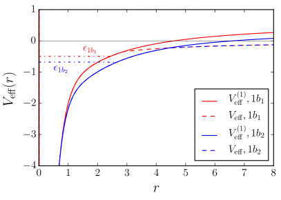
Figure 2: Electronic effective potential in atomic units for the $1b_{1}\approx 2p_{x}$ (red) and $1b_{2}\approx 2p_{y}$ (blue) MO’s of the H₂O molecule. The solid lines give the potential as derived from (2) using the SCF orbitals and eigenenergies, while the dashed lines show the potentials after the Latter correction is applied. The dot-dashed lines show the eigenenergies obtained from the Moccia wave functions Moccia (1964c).

II.2 H₂O in an external electric DC field

Now that we have obtained an effective potential to define the field-free Schrödinger equation (2) for an orbital obtained in the SCF method we proceed with the problem of the molecule exposed to a strong DC field.

When an electric field is applied in the $\hat{z}$ direction, $\vec{F}=F_{0}\hat{z}$, the separation-of-variables ansatz as applied to the Schrödinger equation

$$\psi(r,\theta,\phi) = \psi(r,\theta)\exp(im\phi)$$ (4)

leads to a PDE that represents the Stark problem for an H₂O orbital:

$$-\frac{1}{2}\frac{\partial^{2}\psi}{\partial r^{2}}-\frac{1}{2r^{2}}(\frac{\cos\theta}{\sin\theta}\frac{\partial\psi}{\partial\theta}+\frac{\partial^{2}\psi}{\partial\theta^{2}})+(\frac{m^{2}}{2r^{2}\sin^{2}\theta}+V_{\rm{eff}}(r)-E+F_{0}r\cos\theta)\psi = 0.$$ (5)

Here the complex eigenenergy $E$ contains the information about the resonance position (real part), i.e., $E_{R}$ and width $\Gamma$ (imaginary part is $-\Gamma/2$), and may be expressed as

$$E = E_{R}+iE_{I}=E_{R}-i\frac{\Gamma}{2},$$ (6)

The imaginary part $\Gamma$ is related to the lifetime of the decaying state $\tau$ via $\Gamma\tau=1$. For the $1b_{1}$ and $1b_{2}$ orbitals we have $m=\pm 1$ respectively. The presence of the effective potential $V_{\rm{eff}}(r)$ makes this problem challenging in the sense that it is not possible to obtain separable solutions, as for the hydrogen atom in which a pure Coulomb potential leads to separability in parabolic coordinates Telnov (1989). It is then necessary to generate a more general solution by solving the PDE numerically, e.g., by applying a finite-element method.

II.3 Exterior complex scaling

The ionization regime of the water molecule will be described by means of a non-hermitian Hamiltonian that reveals discrete resonance eigenvalues containing information about the quasi-bound states that tunnel through the barrier or escape over the potential barrier for strong fields. Among the different techniques implemented to compute the resonance energies established methods are the complex scaling Aguilar and Combes (1971); Baslev and Combes (1971); Simon (1973), and exterior complex scaling Simon (1979); the latter was introduced as an extension of the former method. These have been widely used in scattering problems Baslev and Combes (1971); Simon (1973), and also in time-dependent Schrödinger equation problems for strong fields He et al. (2007); Tao et al. (2009); Scrinzi (2010). For our aim of studying the field ionization properties of H₂O orbitals, we implement a modified exterior complex scaling technique in which the radial coordinates are extended into the complex plane by a phase factor, which is turned on gradually beyond some distance from the origin. This method allows to address the tunneling and over-barrier ionization problem by avoiding the complication of describing quasi-bound states with outgoing waves for $r\to\infty$.

In the present work the complex scaling transformation is given by

$$r \rightarrow r\exp(i\chi(r)),$$ (7)

where $\chi(r)$ is defined as a function of the $r$ coordinate with the purpose of making the scaling gradually effective from some vicinity of $r=r_{\rm{s}}$ on,

$$\chi(r) = \frac{\chi_{\rm{s}}}{1+\exp[-\frac{1}{\Delta r}(r-r_{\rm{s}})]}.$$ (8)

For given $r_{s}$ one has to choose $\Delta r$ sufficiently small, so that the function $\chi(r)$ starts from small values at $r=0$. For large $r$ it reaches the value $\chi_{\rm{s}}$.

The set of possible values for the asymptotic scaling angle $\chi_{\rm{s}}$ and the parameters $r_{s}$ and $\Delta r$, which control where and how quickly the scaling is turned on, was explored in detail in order to establish how sensitive the PDE solutions are, and to test the effectiveness of the complex scaling technique to absorb the outgoing wave. Numerous tests were carried out to ensure that the “exact” results of Telnov Telnov (1989) for atomic hydrogen orbitals including $2p$ were reproduced.

In order to investigate the effects of the DC field on the H₂O orbital energies it is necessary to consider the extra terms that the exterior complex scaling (7) introduces in the Schrödinger equation (5). Aditionally, we need to turn the scaling on only in the regime $r>r_{0}$ (Eq. (3)) such that we have a simple Coulomb potential in the scaling region. In order to make use of standard finite element methods, the complex-valued wave function is separated into real and imaginary parts, such that a system of coupled differential equations is obtained as follows:

$$-\frac{1}{2}\frac{\partial^{2}\psi_{R}}{\partial r^{2}}-\frac{1}{2r^{2}}(\frac{\cos\theta}{\sin\theta}\frac{\partial\psi_{R}}{\partial\theta}+\frac{\partial^{2}\psi_{R}}{\partial\theta^{2}})$$

$$+(\frac{m^{2}}{2r^{2}\sin^{2}\theta}+V_{\rm{eff}}^{R}(r)c_{2}-V_{\rm{eff}}^{I}(r)s_{2}-E_{R}c_{2}+E_{I}s_{2}+F_{0}r\cos\theta c_{3})\psi_{R}$$

$$+(-V_{\rm{eff}}^{R}(r)s_{2}-V_{\rm{eff}}^{I}(r)c_{2}+E_{R}s_{2}+E_{I}c_{2}-F_{0}r\cos\theta s_{3})\psi_{I} = 0,$$

$$\vspace{1cm}-\frac{1}{2}\frac{\partial^{2}\psi_{I}}{\partial r^{2}}-\frac{1}{2r^{2}}(\frac{\cos\theta}{\sin\theta}\frac{\partial\psi_{I}}{\partial\theta}+\frac{\partial^{2}\psi_{I}}{\partial\theta^{2}})$$

$$+(\frac{m^{2}}{2r^{2}\sin^{2}\theta}+V_{\rm{eff}}^{R}(r)c_{2}-V_{\rm{eff}}^{I}(r)s_{2}-E_{R}c_{2}+E_{I}s_{2}+F_{0}r\cos\theta c_{3})\psi_{I}$$

$$+(V_{\rm{eff}}^{R}(r)s_{2}+V_{\rm{eff}}^{I}(r)c_{2}-E_{R}s_{2}-E_{I}c_{2}+F_{0}r\cos\theta s_{3})\psi_{R} = 0.$$ (9)

The labels $R(I)$ stand for real and imaginary parts respectively, also the notation $\{c_{k},s_{k}\}$ is introduced to represent $\{\cos(k\chi(r)),\sin(k\chi(r))\}$ respectively, with $k=2,3$ and $\chi(r)$ given in (8).

The PDE system (9) is solved numerically on a rectangular mesh defined by the $(r,\theta)$ coordinates, which take values in the domains $[\epsilon,r_{\rm{max}}]$ and $[\eta,\pi-\eta]$, respectively. The parameters $\epsilon$ and $\eta$ that define the coordinate ranges, were chosen to be of the order of $10^{-3}\ \rm{a.u.}$, and the $r-$coordinate extends to $r_{\rm{max}}=20\ \rm{a.u.}$ In order to find a correct set of $\psi_{R(I)}(r,\theta)$ solutions it is essential to impose proper boundary conditions that ensure the wave functions vanish at the limits of the mesh. For the $|m|=1$ states we impose the condition $\psi_{R(I)}(\epsilon,\theta)=\epsilon\sin(\theta)=\epsilon P_{1}^{1}(\theta)$ which is consistent with the assumption that at small $r=\epsilon$ the lowest term in an expansion in associated Legendre polynomials dominates and behaves like $Ar^{2}\sin(\theta)$.

We implemented a two-parameter root search for $\{E_{R},E_{I}\}$ by solving the PDE as if it were an inhomogeneous problem. We pick a location in the $(r,\theta)$ plane where the probability amplitude is expected to be large and vary $\{E_{R},E_{I}\}$, i.e., effectively the complex energy $E$ to maximize the amplitude.

III Stark resonance parameters

We explored the influence of a set of parameters involved in the 2D problem (9) on the eigenvalue $E_{R}+iE_{I}$ which describes the ionization process as an exponential decay in time in terms of resonance position and half-width. In addition to testing the code against known results for atomic hydrogen Telnov (1989), we have performed systematic studies of our results for the H₂O orbitals against a number of parameters in order to assess the accuracy of these results. One parameter concerns the limiting resolution with which the finite-element method proceeds (the MaxCellSize parameter in the Mathematica10 implementation of NDSolve, which we call $\Delta$). For values $\Delta<0.02\ \rm{a.u.}$ we find stability in the eigenvalues (real and imaginary parts) of two-three significant digits. For the results quoted below we then applied the more stringent criterion of $\Delta=0.01\ \rm{a.u.}$

The second parameter which was investigated is the range where the complex scaling function sets in, i.e., $r_{s}$ and $\Delta r$ in Eq. (8). For the scaling method to work we require scaling to set in for $r>r_{0}$ when the effective potential represents a simple Coulomb tail, which in practice is satisfied by $r_{s}>2r_{0}$. We also need $\Delta r<2\ \rm{a.u.}$ to guarantee smooth turn-on in this region. Small values of $\Delta r$ pose challenges for the automated finite-element method, since in the limit of $\Delta r\to 0$ one would need to implement the derivative discontinuity in the solution as discussed by Scrinzi Scrinzi (2010). We find stable results for the real and imaginary parts of the eigenenergies at the level of three significant digits for the range $10<r_{s}<15\ \rm{a.u.}$ Larger values would require an increase in the computational domain beyond $r=20\ \rm{a.u.}$

Finally, another systematic that was explored is the choice of the ultimate scaling angle reached at large $r$, namely the value of $\chi_{\rm{s}}$ in (8). For an accuracy demand of three significant digits, and the other parameters chosen in the ranges described above stability in the resonance widths is achieved for $0.6<\chi_{\rm{s}}<1.2$ radians.

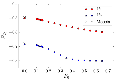
Figure 3: Resonance position in atomic units as a function of the external field strength $F_{0}$ in atomic units for the $1b_{1}$ (red circles) and $1b_{2}$ (blue triangles) MO’s of H₂O.

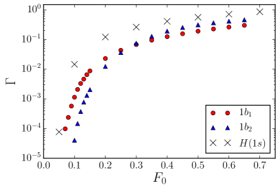
Figure 4: Resonance width in atomic units as a function of the external field strength $F_{0}$ in atomic units for the $1b_{1}$ (red circles) and $1b_{2}$ (blue triangles) MO’s of H₂O. For comparison, atomic hydrogen H($1s$) ionization rates from Refs. Telnov (1989); Kolosov (1987) are shown as crosses.

In Fig. 3 we show the resonance position $E_{R}$ as obtained from the present calculations for the weakly bound $1b_{1}$ and the strongly bound $1b_{2}$ valence orbitals as a function of applied electric field strength $F_{0}$. In the limit of zero field the calculation reproduces the SCF eigenvalues of Moccia Moccia (1964c). The field has to be strong (in comparison with atomic hydrogen results for $2p$ orbitals Telnov (1989)) in order to change the resonance position appreciably. For the more deeply bound $1b_{2}$ orbital the shift in resonance position saturates with field strength.

In Fig. 4 the resonance widths are shown for both orbitals as functions of external field strength $F_{0}$. The graphs display threshold behavior at the weaker field strengths. As expected we find a lower threshold (critical field strength) for the more weakly bound $1b_{1}$ orbital. Interestingly, however at a field strength of about $F_{0}=0.3\ \rm{a.u.}$ the values for the widths cross, i.e., the deeper bound $1b_{2}$ orbital displays a larger ionization rate as the field strength is increased further.

Also shown in Fig. 4 are the widths for the H($1s$) orbital from Refs. Telnov (1989); Kolosov (1987). They can be compared to the $1b_{1}$ orbital results, since the binding energy is very close in the free-field limit. Since the tunneling barrier is mostly in the asymptotic regime where the potential energy has a $-1/r$ tail, it is not surprising that the widths for H₂O($1b_{1}$) and H($1s$) share some similarity in shape. In the tunneling region H($1s$) has an ionization rate that is larger by about an order of magnitude. In the over-barrier regime, however, the ionization rates come to within a factor of 3. Reasons for why he $1b_{1}$ water molecular orbital is harder to ionize than H($1s$) have to do with the different shape of the orbital density ($m=1$ vs the spherical H($1s$) density), and the substantially more attractive potential at shorter distances.

An examination of contour plots of the densities $\Psi^{*}\Psi$, as well as of the potential energies $V_{\rm{eff}}(r)-F_{0}z$ for different field strengths, (both as a function of $r,\theta$), allows to make the following observations. For field strengths $F_{0}<0.1\ \rm{a.u.}$ there is a barrier the electrons need to penetrate in order to be ionized. From the potential energy plot shown in Fig. 3 one can see that for weak fields (small values of $F_{0}$) the barrier is longer for the more deeply bound $1b_{2}$ orbital. This explains why the ionization threshold occurs for $F_{0}>0.1\ \rm{a.u.}$ for this orbital, which is about a factor of two larger than for the $1b_{1}$ orbital.

The field strength region where the ionization rates (resonance widths) display a change in character, i.e., turn over to rise much more gradually with the field strength $F_{0}$ can be characterized as a regime where there is a narrow potential saddle at small $\theta$, in the vicinity of $r\approx 3\ \rm{a.u.}$, such that electron flux can leave, and is then accelerated by the electric field. The crossing of the ionization rates for the $1b_{1}$ and $1b_{2}$ orbitals occurs, since the saddle in the potential becomes effectively lower at strong fields for the $1b_{2}$ orbital. This can be inferred from the comparison of the two effective potentials, which share the same asymptotic behavior beyond $r=4.3\ \rm{a.u.}$ (see Figure 2).

The origin for the different radial dependencies of the effective potential for the two orbitals can be found in the geometry of the water molecule. The weakly bound $1b_{1}$ orbital has its lobes perpendicular to the plane defined by the location of the three nuclei. Therefore, it is least affected by the two protons. The $1b_{2}$ orbital explores the potentials due to the protons more strongly in the SCF calculation of Moccia, and, therefore, the resulting (in our approximation spherically symmetric) $V_{\rm{eff}}(r)$ has a more attractive region in the range $0.7<r<4.3$.

Table 1: Resonance positions and widths for different field strengths in atomic units. The numbers in brackets indicate the exponent $k$, i.e., the numbers are to be multiplied by $10^{k}$.

		$1b_{1}$		$1b_{2}$
$F_{0}$	$E_{R}$	$\Gamma$	$E_{R}$	$\Gamma$
$0.1$	$-0.506$	$1.14(-3)$	$-0.689$	$4.04(-5)$
$0.2$	$-0.525$	$2.28(-2)$	$-0.718$	$1.23(-2)$
$0.3$	$-0.546$	$6.74(-2)$	$-0.760$	$7.51(-2)$
$0.4$	$-0.564$	$1.24(-1)$	$-0.790$	$1.91(-1)$
$0.5$	$-0.580$	$1.90(-1)$	$-0.796$	$3.11(-1)$
$0.6$	$-0.593$	$2.61(-1)$	$-0.797$	$4.11(-1)$

We summarize the results in Table 1 for further reference, i.e., for future comparison with calculations based on other models for the molecular orbitals.

IV Conclusion

We have carried out a study of two of the three valence orbitals of the water molecule, $1b_{1}$ and $1b_{2}$, in the presence of an external electric DC field. The tunneling ionization and over-barrier ionization regimes were explored by finding a numerical solution to the PDE system defined by an effective potential obtained from single-center Slater-type orbitals. The exterior complex scaling parameters as well as a finite-element resolution parameter were optimized to guarantee a minimum of $2-3$ significant digits for the solutions. The resonance parameters that describe the ionization process, resonance position and width, were explored over a wide range of electric field strengths. We demonstrated how an increase of the field strength beyond a critical point in the over-barrier region led to a crossing between the ionization rates of the two orbitals. Additional observations of the effective potential for different field strengths were carried out to shed some light on the interpretation of this behavior.

References

- Murakami et al. (2012a) M. Murakami, T. Kirchner, M. Horbatsch, and H. J. Lüdde, Phys. Rev. A 85, 052713 (2012a).
- Murakami et al. (2012b) M. Murakami, T. Kirchner, M. Horbatsch, and H. J. Lüdde, Phys. Rev. A 86, 022719 (2012b).
- Luna et al. (2016) H. Luna, W. Wolff, E. C. Montenegro, A. C. Tavares, H. J. Lüdde, G. Schenk, M. Horbatsch, and T. Kirchner, Phys. Rev. A 93, 052705 (2016).
- Gulyás et al. (2016) L. Gulyás, S. Egri, H. Ghavaminia, and A. Igarashi, Phys. Rev. A 93, 032704 (2016).
- Hong et al. (2016) X. Hong, F. Wang, Y. Wu, B. Gou, and J. Wang, Phys. Rev. A 93, 062706 (2016).
- Errea et al. (2013) L. F. Errea, C. Illescas, L. Méndez, and I. Rabadán, Phys. Rev. A 87, 032709 (2013).
- Nandi et al. (2013) S. Nandi, S. Biswas, A. Khan, J. M. Monti, C. A. Tachino, R. D. Rivarola, D. Misra, and L. C. Tribedi, Phys. Rev. A 87, 052710 (2013).
- Farrell et al. (2011) J. P. Farrell, S. Petretti, J. Förster, B. K. McFarland, L. S. Spector, Y. V. Vanne, P. Decleva, P. H. Bucksbaum, A. Saenz, and M. Gühr, Phys. Rev. Lett. 107, 083001 (2011).
- Falge et al. (2010) M. Falge, V. Engel, and M. Lein, Phys. Rev. A 81, 023412 (2010).
- Tsogbayar and Horbatsch (2013a) T. Tsogbayar and M. Horbatsch, Journal of Physics B: Atomic, Molecular and Optical Physics 46, 085004 (2013a).
- Chu and Chu (2000) X. Chu and S.-I. Chu, Phys. Rev. A 63, 013414 (2000).
- Plummer and McCann (1996) M. Plummer and J. F. McCann, Journal of Physics B: Atomic, Molecular and Optical Physics 29, 4625 (1996).
- Tsogbayar and Horbatsch (2013b) T. Tsogbayar and M. Horbatsch, Journal of Physics B: Atomic, Molecular and Optical Physics 46, 245005 (2013b).
- Werner et al. (1995) U. Werner, K. Beckord, J. Becker, and H. O. Lutz, Phys. Rev. Lett. 74, 1962 (1995).
- Gobet et al. (2001) F. Gobet, B. Farizon, M. Farizon, M. J. Gaillard, M. Carré, M. Lezius, P. Scheier, and T. D. Märk, Phys. Rev. Lett. 86, 3751 (2001).
- Gobet et al. (2004) F. Gobet, S. Eden, B. Coupier, J. Tabet, B. Farizon, M. Farizon, M. J. Gaillard, M. Carré, S. Ouaskit, T. D. Märk, and P. Scheier, Phys. Rev. A 70, 062716 (2004).
- Luna et al. (2007) H. Luna, A. L. F. de Barros, J. A. Wyer, S. W. J. Scully, J. Lecointre, P. M. Y. Garcia, G. M. Sigaud, A. C. F. Santos, V. Senthil, M. B. Shah, C. J. Latimer, and E. C. Montenegro, Phys. Rev. A 75, 042711 (2007).
- Aung et al. (1968) S. Aung, R. M. Pitzer, and S. I. Chan, The Journal of Chemical Physics 49, 2071 (1968).
- Moccia (1964a) R. Moccia, The Journal of Chemical Physics 40, 2164 (1964a).
- Moccia (1964b) R. Moccia, The Journal of Chemical Physics 40, 2176 (1964b).
- Moccia (1964c) R. Moccia, The Journal of Chemical Physics 40, 2186 (1964c).
- Montanari and Miraglia (2014) C. C. Montanari and J. E. Miraglia, Journal of Physics B: Atomic, Molecular and Optical Physics 47, 015201 (2014).
- Hafied et al. (2007) H. Hafied, A. Eschenbrenner, C. Champion, M. F. Ruiz-López, C. D. Cappello, I. Charpentier, and P. A. Hervieux, Chemical Physics Letters 439, 55 (2007).
- Ning et al. (2008) C. G. Ning, B. Hajgató, Y. R. Huang, S. F. Zhang, K. Liu, Z. H. Luo, S. Knippenberg, J. K. Deng, and M. S. Deleuze, Chemical Physics 343, 19 (2008).
- Roothaan (1951) C. C. J. Roothaan, Reviews of Modern Physics 23, 69 (1951).
- Latter (1955) R. Latter, Phys. Rev. 99, 510 (1955).
- Telnov (1989) D. A. Telnov, J. Phys. B: At. Mol. Opt. Phys. 22, L399 (1989).
- Aguilar and Combes (1971) J. Aguilar and J. M. Combes, Commun. Math. Phys. 22, 269 (1971).
- Baslev and Combes (1971) E. Baslev and J. M. Combes, Commun. Math. Phys. 22, 280 (1971).
- Simon (1973) B. Simon, Ann. Math. 97, 247 (1973).
- Simon (1979) B. Simon, Phys. Rev. Lett. 71A, 211 (1979).
- He et al. (2007) F. He, C. Ruiz, and A. Becker, Phys. Rev. A 75, 053407 (2007).
- Tao et al. (2009) L. Tao, W. Vanroose, B. Reps, T. N. Rescigno, and C. W. McCurdy, Phys. Rev. A 80, 063419 (2009).
- Scrinzi (2010) A. Scrinzi, Phys. Rev. A 81, 053845 (2010).
- Kolosov (1987) V. V. Kolosov, J. Phys. B: At. Mol. Opt. Phys. 20, 2359 (1987).